Abstract
Rationale and Objectives
To develop and validate an automated method to segment renal cortex on contrast-enhanced abdominal CT images from kidney donors, and to track the cortex volume change after donation.
Materials and Methods
A 3D fully automated renal cortex segmentation method was developed and validated on 37 arterial phase CT data sets (27 patients, 10 of them had two CT scans before and after nephrectomy) using leave-one-out strategy. Two expert interpreters manually segmented the cortex slice-by-slice, the linear regression analysis and Bland-Altman plots were used to compare the automated and manual segmentations. The true positive and false positive volume fractions were also calculated to evaluate the accuracy of the proposed method. Volume changes of cortex for 10 subjects were also calculated.
Results
The linear regression analysis results showed Auto and manual methods had strong correlations with Pearson correlation value of 0.9529, 0.9309, 0.9283 and 0.9124 between intra-observer variations, inter-observer variations, Auto and User1, and Auto and User2, respectively (p<0.001 for all the analysis). The Bland-Altman plots for cortex segmentation also showed Auto and manual methods had agreeable segmentation. The mean volume increase of the cortex for the 10 subjects was 35.1%±13.2% (p<0.01 by paired t-test). The overall true positive and false positive volume fractions for cortex segmentation were 90.15 ± 3.11% and 0.85 ± 0.05%. With the proposed automatic method, the time for cortex segmentation was reduced from 20 minutes of manual segmentation time to 2 minutes.
Conclusions
The proposed method was accurate and efficient and can replace the current subjective and time-consuming manual procedure. The computer measurement confirms the volume of renal cortex increases after kidney donation.
Keywords: Kidney, Renal Cortex, Automatic Renal Cortex Segmentation, Kidney Donors
INTRODUCTION
The renal cortex, the outer kidney layer consisting of renal corpuscles and convoluted tubules, has distinct morphology and function from the inner renal medulla. Because glomerular filtration, an important clinical assessment of renal function, is the main function of the renal cortex, there has been a considerable interest in accurately assessing the renal cortical size and volume. The current method for renal cortex segmentation in clinics, however, is mainly operated manually [1–6] which is subjective and tedious. There were several prior investigations [7–14] in renal cortex segmentation on CT and MRI images, including both semi-automatic [8, 10, 11, 12] and fully automatic [7, 9, 13, 14] methods. However, most of these studies considered renal cortex and renal column as one tissue type although they are anatomically different. In this paper, we propose a method to precisely and automatically segment the renal cortex. To the best of our knowledge, this study is the first work that aims to automatically separate the renal cortex and renal column in the renal segmentation.
In kidney transplantation, the ability to accurately and reliably measure renal volume may give clinicians better understanding of the aftereffect of kidney donation and therefore improve the kidney donor selection process. Limited but available data suggests that larger renal volume is associated with better renal graft function in the recipients one year after the transplantation [15]. A few studies [12–16] have estimated the kidney volume change after the donation by using image findings (such as CT, MRI and Ultrasound). In this investigation, we also track the volume change of the cortex for the remaining kidney of the donors. As for the volume change in renal cortex, to the best of our knowledge, we are the first one to measure the change after donation.
MATERIALS AND METHODS
Donors
Approval for this retrospective study was obtained from our Institutional Review Board, which waived the requirement for informed consent. This study was compliant with the Health Insurance Portability and Accountability Act.
Between 1999 and 2006, 108 patients had undergone kidney donation at our institution. In order to obtain comprehensive clinical evaluation, all donors were invited to participate in a follow-up study. Out of 108, 52 donors returned for clinical and laboratory exams and detailed interviews. Of the 52, we limited our study to those who had contrast-enhanced CT images and excluded those who had MR imaging. This yielded 29 patients. Among these 29 patients, 27 donated left kidney (right kidney was imaged), and 2 donated right kidney (we excluded them since the number was too small to build the anatomical model). Among the 27 subjects left in this study, there were 7 men and 20 women, with a median age of 46 years (mean age, 44 years ± 11 [standard deviation]; range, 19 – 63 years) at the donation time. Among these 27 subjects, 10 had both contrast-enhanced CT images before and after nephrectomy. The median interval between the baseline and follow-up CT examinations for these 10 patients was 1564 days (range, 895–2181 days).
CT Imaging
Abdominal images were acquired during preoperative screening. All examinations were performed with one of two different types of CT scanners (GE Medical systems, LightSpeed Ultra and Philips, Mx8000 IDT 16). Prior to the image acquisition, the patients were injected with 130ml of ISOVUE-300 contrast agent. CT images were reviewed with a 3D multi-planar reformatting interactive mode on an image processing workstation (Advanced Workstation; GE Healthcare). The integrated workstation allows the reader to draw contours and regions of interest and automatically calculates the area enclosed by the region of interest. The slice thickness ranged from 1 to 5 mm. The in-plane pixel size ranged from 0.63 to 0.88 mm. The distribution of the data is as follows: in a total of 37 images, there are 10, 12 and 15 images with in-plane pixel size × slice thickness of 0.63×0.63×1, 0.71×0.63×2 and 0.88×0.88×5 mm3, respectively.
Documented information included patient age at diagnosis and date of surgery. The examination date, section thickness, and section spacing were also recorded.
Manual Segmentation
Two independent trained observers (radiology CT technologist User1 and User2, both had more than 5 years of experience with kidney CT imaging): User1 performed manual segmentations for each patient twice with the duration of 3 months, and User2 performed manual segmentations only once. To prevent bias, the observers were blinded to the results of the other observer. The segmentations were performed using GE AWS thin-client server. They manually drew the contour on the cortex boundaries to get the outer-layer and inner-layer contour in a slice-by-slice mode. Then the tissues between the two layers are identified as cortex. The total volumes of the cortex were obtained by summing all the voxel volumes lying within the boundaries. The total segmentation time was also recorded.
Automatic Segmentation
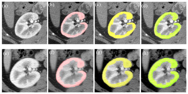
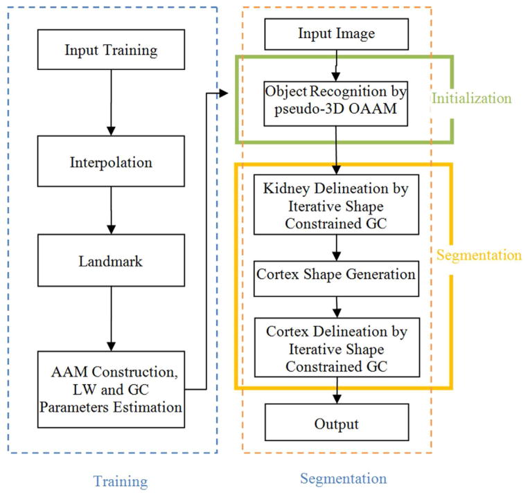
The segmentation of the renal cortex is not a trivial task. As shown in Fig. 4(a), the main challenge in separating the cortex from the rest of the kidney is their quite similar intensity profiles; therefore, it is hard to separate them only based on intensity features. The kidney shape could provide necessary constraints. Hence, in this paper, we propose a 3D shape-constrained graph cut (GC) method [23, 24] to solve this problem. The GC methods have been used widely and achieved good performance [23]. Then how to get the 3D shape constraint becomes essential for the whole method. We proposed to use the OAAM method to get the shape constraints. OAAM effectively combines the active appearance model (AAM) [21, 25] and live wire (LW) [22] methods. The proposed method consists of three main parts: model building (training), kidney initialization, and renal cortex segmentation, as shown in Figure 1. Details for each part are given as follows.
Figure 4.
Examples of segmentation results for cortex segmentation. The first and second rows show the corresponding slices before and after nephrectomy, respectively. (a) One slice image before nephrectomy; (b) User1 segmentation results on (a); (c) User2 segmentation results on (a); (d) Automatic segmentation results on (a); (e) The corresponding slice image after nephrectomy of (a); (f) User1 segmentation results on (e); (g) User2 segmentation results on (e); (h) Automatic segmentation results on (e).
Figure 1.
The flowchart of the proposed cortex segmentation system.
(1) Model Building and Training
During the model building (training) step, there are three main steps: (i) Manually specify landmarks on the training shapes; (ii) Construct an active appearance model; (iii) Parameters estimation for LW and GC methods based on the training data set.
Landmark Specification
Due to the nature of the proposed method (slice by slice), we represent a 3D shape as a stack of 2D contours, and manually label the 3D shape slice by slice. For each slice, operators locate the shape visually, and then identify prominent landmarks on that shape.
AAM Construction
The conventional AAM method [21, 25] is used for constructing the model. The model includes both shape and texture information.
Suppose Mj represents the AAM for slice level j and the number of slice levels is n, then the total model M can be represented as
| (1) |
Although we employ the pseudo 3D initialization strategy, we also build the real 3D AAM M3D using the method in [21]. However, this 3D model M3D is used only for providing the delineation constraints as explained later.
Parameters Estimation
In the proposed method, the initialization is implemented by multi-object oriented active appearance model (OAAM) method which combines the AAM with LW methods. The delineation is accomplished by shape constrained GC method. During the training stage, the parameters for LW are trained per LW method [22] from the training data set. And the parameters estimation for GC is given in the below.
(2) Kidney Initialization
The initialization step plays an important role in the overall framework. It not only provides shape constraints to the later GC segmentation, but also makes the whole method fully automated. The proposed initialization method includes three main steps. First, a slice localization method is applied to detect the top and bottom slices of the kidney. After the localization of the top and bottom slices, all the slices in between are linearly interpolated into 32 slices same as in the AAM model construction process. Second, the organ is recognized slice by slice via a multi-resolution OAAM method. A multi-object strategy [26] is utilized to further assist the kidney initialization. Finally, after objects are recognized in all slices, the recognized shapes are stacked together to form 3D initialization result. In the initialization method, the second step is the key for the success of the whole initialization. More details are given as follows.
Localization of Top and Bottom Slices
The aim here is to locate the top and bottom slices of the kidney. Since we already trained a model for each organ slice, we could use this model for slice localization. The proposed method is based on the similarity to the top/bottom slice’s OAAM model. For top slice localization in a given image, the top slice model is applied to each slice in the image using the recognition method detailed in the following sub-section, and evaluate the respective similarity metric (Eqn. (2)). Then the slice corresponding to the maximum similarity is taken as the top slice of the organ. For the bottom slice detection, a similar method is used.
Oriented Active Appearance Model
The conventional AAM matching method for object recognition is based on the root-mean-square difference between the appearance model instance and the target image. Such a strategy is better suited for matching appearances than for the detailed segmentation of target images. This is because the AAM is optimized on global appearance, and is thus, less sensitive to local structures and boundary information. Conversely, the LW delineates the boundary very well [22], however it needs a good initialization of landmarks and is an interactive method. Here, we integrate the AAM with the LW method (termed OAAM) to combine their complementary strengths. That is, the AAM provides the landmarks to the LW, and in return, LW improves the shape model of the AAM. The LW is fully integrated with AAM in two aspects: (1) LW is used to refine the shape model in AAM; (2) the LW boundary cost is integrated into cost computation during the AAM optimization method.
In the conventional AAM optimization method, the optimization is based only on the difference between the appearance model instance and the target image. The boundary cost is not taken into consideration. By combining the boundary cost, the performance of AAM matching can be considerably improved. In the proposed method, the LW technique is integrated into the cost computation during the optimization process. Given a current estimate of the model parameters b, the post t, the texture transformation u, and the image sample at the current estimate gim, our optimization method is as follows.
OAAM Optimization Algorithm
Project the texture sample into the texture model frame using .
-
Evaluate the errors:
Texture error Eaam = |r(φ)|2, where φT = (bT|t′T|uT) and r(φ) = gs′ − gim′.
Total error by combining Eaam and LW cost along the shape boundary Elw,(2) Compute the predicted displacements δφ = −Rr(φ), where .
Set k = 1,
Update the parameters φ ← φ + kδφ,
Based on the new parameters φ, repeat steps 1–3, and get the new error .
-
If , then accept the new parameters and go to step 8.
Else try k = 0.5, 0.25, etc. and go to step 5.
Repeat starting with step 1 until no improvement is made to the total error.
(3) Renal Cortex Segmentation
The shape constrained GC methods is the building block of the proposed renal cortex segmentation algorithm, we presented it first.
Shape constrained GC
The segmentation problem can be formulated as an energy minimization problem such that for a set of pixels P and a set of labels L, the goal is to find a labeling f: P → L that minimizes the energy function,
| (3) |
where Np is the set of pixels in the neighborhood of p, Rp (fp) is the cost of assigning label fp ∈ L to p, and Bp,q (fp, fq) is the cost of assigning labels fp, fq ∈ L to p and q.
In our framework, the unary cost Rp(fp) is the sum of a data penalty Dp(fp)and a shape penalty Sp (fp) term. The data term is defined based on the image intensity and can be considered as a log likelihood of the image intensity for the target object. The shape prior term is independent of image information, and the boundary term Bp,q is based on the gradient of the image intensity.
The proposed shape-integrated energy function is defined as follows:
| (4) |
where α, β, γ are the weights for the data term, shape term Sp, and boundary term, respectively, satisfying α + β + γ = 1. These components are defined as follows:
| (5) |
| (6) |
| (7) |
where Ip is the intensity of pixel p, object label, is the label of the object (foreground). P(Ip | O) and P(Ip|B) are the probability of intensity of pixel p belonging to object and background respectively, which are estimated from object and background intensity histograms during the training phase (details given below). d(p, q) is the Euclidian distance between pixels p and q, and σ is the standard deviation of the intensity differences of neighboring voxels along the boundary.
| (8) |
where d ( p, xO) is the distance from pixel p to the set of pixels which constitute the interior of the current shape xo of object O. (Note that if p is in the interior of xo, then d (p, xO) = 0.) d (p, x̄o) is the distance from voxel p to the complementary of the shape xo. rO is the radius of the sphere that roughly encloses xo. The linear time method of reference [31] was used in this paper for computing this distance.
During the training stage, the intensity histogram of each object is estimated from the training images. Based on this, P(Ip|O) and P(Ip|B) can be computed. As for parameters α, β and γ in Eqn. (4), since α + β + γ = 1, we estimate only α and β by optimizing accuracy as a function of α and β and set γ = 1 − α − β. We use the gradient descent method for the optimization. Accu (α, β) represents the algorithm’s accuracy (here we use the true positive volume fraction [30]). α and β are initialized to 0.35 each, and Accu (α, β) is optimized over the training data set to determine the best α and β.
Renal Cortex Segmentation
The proposed renal cortex segmentation method consists of three main steps. First, the kidney is segmented using the iterative shape constrained GC method which incorporated the kidney shape information generated from the initialization step. Second, after getting the kidney contour, morphological operations (five times erosion followed by image subtraction) are applied to it to get the initial cortex shape. Finally, the renal cortex is segmented by using the iterative shape constrained GC method. At this time, the initial cortex shape result is used as a constraint. The iterative shape constrained GC method is given as follows.
Perform GC segmentation minimizing Eqn. (3) using the available shape constraints;
Compute the new position of the landmarks by moving each landmark in the shape to the point closest on the GC boundary;
-
If no landmarks moved or the distance between two shapes is less than pre-defined threshold thr, then the converge is assumed, and go to step 4;
Else subject the shape result to the constraint of model M3D and update it as the new shape constraints, and go to step 1.
Perform one final GC segmentation based on the latest shape constraints, and obtain the associated object boundaries.
In our implementation, thr is set as 1 unit, and for shape update constraints, we limit the distance each voxel on the surface can move within any iteration to 6 units, this will make the shape change smoother.
Statistical Analyses and Segmentation Evaluation
The linear regression analysis [27] and Bland-Altman plots [28, 29] were used to evaluate the correlations and agreements between the automated and manual segmentations. The analysis of between intra-observer variations (User1 two segmentations), inter-observer variations (User1 and User2), Auto and User1, and Auto and User2 were performed. The median, mean and standard deviation of the cortex volume change for the remaining kidney before and after the donation were also calculated.
The true positive and false positive volume fractions (TPVF and FPVF) [30] were also calculated to evaluate the accuracy of the proposed segmentation method. TPVF indicates the fraction of the total amount of tissue in the true delineation; FPVF denotes the amount of tissue falsely identified, which are defined as follows,
| (9) |
| (10) |
Where, CTP is the set of voxels in the true positive delineation, Ctd is the set of voxels in the ground truth, CFP is the set of voxels in the falsely identified, Ud is assumed to be a binary scene with all voxels in the scene domain, and |·| denotes volume.
The proposed method was evaluated using “leave-one-out” strategy. Here, one means “one patient”. In total, we have 37 images from 27 patients (10 of them had two CT scans before and after nephrectomy). When the tesing image is of a patient who has only one image, the remaining 36 images will be used for training; while when the testing image is of a patient who has two images, the remaining 35 images will be used for training.
RESULTS
Correlations between Manual and Automatic Segmentation
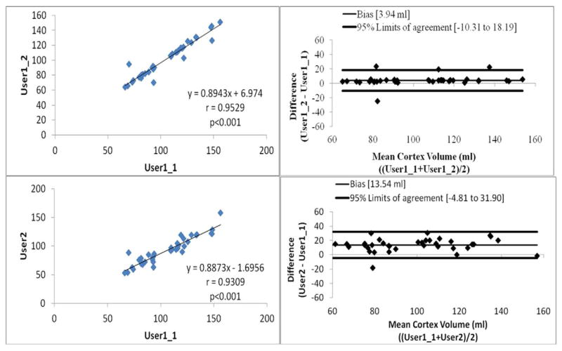
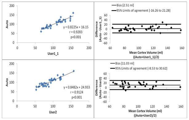
The linear regression analysis (Figures 2 and 3) showed that Pearson correlation were 0.9529, 0.9309, 0.9283 and 0.9124 between intra-observer variations, inter-observer variations, Auto and User1, and Auto and User2, respectively (p<0.001 for all the analysis). The Bland-Altman plots (Figures 2 and 3) showed that the 95% limits of agreement were [−10.31, 18.19], [−4.81, 31.90], [−16.26, 21.28] and [−8.53, 30.62] (ml), between intra-observer variations, inter-observer variations, Auto and User1, and Auto and User2, respectively. We can see that the correlation analysis results showed Auto had strong correlations with both of manual segmentation results. Figure 4 shows examples of cortex segmentation results of User1, User2 and automatic method, and the 3D visualization results.
Figure 2.
Linear regression analysis and Bland-Altman plots for intra-observer and inter-observer assessment of manual segmentation results.
Figure 3.
Linear regression analysis and Bland-Altman plots for automatic and manual segmentation results.
Accuracy of Localization of Top and Bottom Slices
The OAAM models of top and bottom slice were used to identify the location of top and bottom slice of the kidney. The kidney was manually checked by an expert to generate the reference standard of top and bottom position. The average localization error ±std. dev. for top and bottom slice is 7.3±5.2 and 6.1±4.5 mm, respectively.
Segmentation Accuracy Measurement
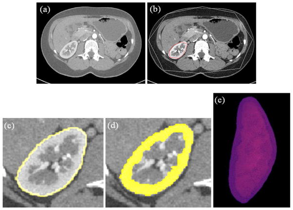
As the correlation analysis results showed Auto had strong correlation with both of manual segmentation results, therefore, the User1 first segmentations (User1_1 in Figure 2) were chosen as references. Figure 5 shows the experimental results for one slice level of kidney and cortex segmentation. The TPVF and FPVF for the kidney segmentation over the whole dataset was 96.32 ± 6.12% and 0.29± 0.05%, respectively (mean ± standard deviation). While for the cortex segmentation, the TPVF and FPVF over the whole dataset was 90.15 ± 3.11% and 0.85 ± 0.05%, respectively. The performance on the training data set was as follows: the TPVF and FPVF for the kidney segmentation were 97.85 ± 5.06% and 0.18± 0.05%, respectively; for the cortex segmentation, 92.89 ± 2.25% and 0.68 ± 0.04%, respectively.
Figure 5.
Experimental results of kidney and cortex segmentation on one slice by the proposed method. (a) Original slice image; (b) Initialization result; (c) Kidney segmentation results (d) Cortex segmentation result; (e) 3D visualization of cortex segmentation result.
Operation Time Evaluation
The running time for each step was recorded, which consists of three parts: initialization time (i.e., the time required to get the initialization results), computing time for kidney segmentation (i.e., the time required to automatically delineate the kidney contours), and computing time for cortex segmentation (i.e., the time required to automatically delineate the cortex contours). The operation time (expressed as means ± standard deviations), for two manual and automatic segmentations, are reported in Table 1. For automatic segmentation, the total time is divided into the time required for kidney initialization, kidney segmentation, and cortex segmentation. For kidney segmentation, the time was reduced from average 8 minutes for manual segmentation, to about 1.3 minutes for automatic segmentation. For cortex segmentation, the time was reduced from average 20 minutes for manual segmentation, to less than 2 minutes for automatic segmentation.
Table 1.
Running time in the segmentation procedures
| Procedure | Time (sec) (mean ± std.dev.) |
|---|---|
| Automatic Segmentation | |
| Step 1: initialization | 40±5 |
| Step 2: kidney segmentation | 35±6 |
| Step 3: cortex segmentation | 30±3 |
| Total | |
| Kidney segmentation (step 1 + step 2) | 75±7 |
| Cortex segmentation (step 1 + step 2 + step3) | 105±8 |
|
| |
| Manual Segmentation – User1 | |
| Kidney segmentation | 435±45 |
| Cortex segmentation | 1152±60 |
|
| |
| Manual Segmentation – User2 | |
| Kidney segmentation | 486±35 |
| Cortex segmentation | 1209±50 |
Volume Change before and after Donation
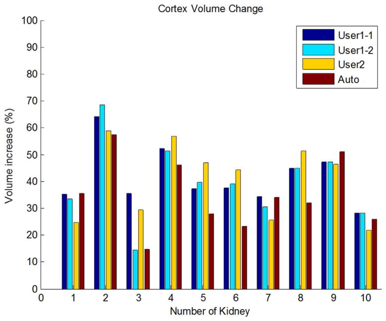
The median volume for cortex of the remaining kidney was 83.4 mL (mean, 82.9 ± 10.7 mL; range, 60.1–96.1 mL) before donation and 113.1 mL (mean, 112.5±14.8 mL; range, 76.8–128.7 mL) after donation based on Auto segmentation results. Figure 4 shows one case of the cortex segmentation (kidney #2 in Figure 6) on one corresponding slices before and after nephrectomy. Figure 6 shows the quantitative results: the median volume increase for renal cortex was 34.1% (mean ± std.dev: 35.1% ± 13.2%; range: 14.6%–57.3%) based on Auto segmentation results. The increase was significant by using paired t-test, p<0.01.
Figure 6.
Renal cortex volume change by User1, User2 and Auto segmentation results.
DISCUSSION
We can see from Figures 2 and 3 that: (1) the intra-observer variations has the highest correlation with Pearson correlation r=0.9529 and inter-observer variations also shows high correlation with r=0.9309. Compare to the correlations of manual segmentations, auto also achieves high correlations with manual segmentations, r=0.9283 for Auto and User1, and r=0.9124 for Auto and User2. (2) For the Bland-Altman plots, the 95% limits of agreement were [−10.31, 18.19] and [−4.81, 31.90] for intra- and inter-observation variations, respectively. Comparing to the manual results, auto and manually has very similar agreement results, 95% limits of agreement were [−16.26, 21.28] and [−8.53, 30.62] for Auto-User1 and Auto-User2, respectively. The proposed automatic method achieved high correlations and agreements with the manual segmentation.
For the accuracy analysis of the proposed segmentation method, the User1 first segmentations were chosen as references, and the high TPVF of 96.32% and 89.15%, and low FPVF of 0.29% and 0.85% were achieved for the kidney and cortex segmentation, respectively. In addition, we also evaluated the proposed segmentation method based on the references of User1’s second and User2’s segmentations to see the performance differences. The TPVF was 96.21 and 90.32 (96.02 and 90.01), and FPVF was 0.36 and 0.92 (0.26 and 0.81) for the kidney and cortex segmentation based on the references of User1’s second (User2’s) segmentations, respectively. We can conclude from the results that, no matter which reference was used, the high TPVF of >96% and >90%, and low FPVF of <0.5% and <1% can be achieved for the kidney and cortex segmentation, respectively. The TPVF (FPVF) of cortex segmentation is lower (higher) than kidney segmentation, which could be due to the greater difficulty in locating cortex inner wall.
Use of the automatic segmentation algorithm greatly reduced the time needed for the renal cortex segmentation. The reduction of the mean segmentation time from about 20 minutes to less than 2 minutes made cortex segmentation at CT imaging more practical in clinics. The segmentation process consists of three steps: initialization, kidney segmentation, and cortex segmentation. The initialization time might be further reduced by using hierarchical, multi-resolution strategy, which can also improve the initialization accuracy. For the kidney and cortex segmentation, we used the iterative shape constrained graph cut method. Here, we set iteration number as three. With a better initialization, the iteration number can also be decreased, which can save additional time.
For the cortex volume change of the remaining kidney before and after donation, all cortex volumes increased based on User1 two segmentations, User2 and Auto segmentations as shown in Figure 6. As the Auto segmentation achieved high correlations with manual segmentation, only the cortex volume change results based on Auto segmentation were given here. Based on Auto segmentation, the average increase of the renal cortex volume was about 35.1%. To the best of our knowledge, this is the first report of the volume change of renal cortex for kidney donors.
Although one limitation in our study is the size of the study sample, we hope the results presented here will serve as a pilot study prompting further studies with larger patient samples to validate the results.
In conclusion, we developed a fully automated technique to segment renal cortex on abdominal contrast-enhanced CT scans. The method was validated on a clinical data set with 37 contrast-enhanced CT images of 27 patients and achieved high correlation with manual segmentations. The use of automatic cortex segmentation method saved substantial amount of time. The proposed technique provides an automated, objective and accurate segmentation of renal cortex, and it can replace the current subjective and time-consuming manual procedure. Other potential further improvements of the technique include the segmentation and measurement of renal medulla and pelvis volumes.
Acknowledgments
Grant Support
This research was supported by the Intramural Program of the National Institutes of Health, Clinical Center.
Footnotes
This paper was presented at RSNA 2010 as a scientific paper.
Potential Conflict of Interest
The authors declare that they have no competing interests.
Publisher's Disclaimer: This is a PDF file of an unedited manuscript that has been accepted for publication. As a service to our customers we are providing this early version of the manuscript. The manuscript will undergo copyediting, typesetting, and review of the resulting proof before it is published in its final citable form. Please note that during the production process errors may be discovered which could affect the content, and all legal disclaimers that apply to the journal pertain.
References
- 1.Lee VS, Rusinek H, Noz ME, Lee P, Raghavan M, Kramer EL. Dynamic three-dimensional MR renography for the measurement of single kidney function: initial experience. Radiology. 2003;227:289–294. doi: 10.1148/radiol.2271020383. [DOI] [PubMed] [Google Scholar]
- 2.Van den Dool SW, Wasser MN, de Fijter JW, Hoekstra J, van der Geest RJ. Functional renal volume: quantitative analysis at gadolinium-enhanced MR Angiography-feasibility study in healthy potential kidney donors. Radiology. 2005;236:189–195. doi: 10.1148/radiol.2361021463. [DOI] [PubMed] [Google Scholar]
- 3.Holden A, Smith A, Dukes P, Pilmore H, Yasutomi M. Assessment of 100 live potential renal donors for laparoscopic nephrectomy with multi–detector row helical CT. Radiology. 2005;237:973–980. doi: 10.1148/radiol.2373041303. [DOI] [PubMed] [Google Scholar]
- 4.Halpern EJ, Mitchell DG, Wechsler RJ, Outwater EK, et al. Preoperative evaluation of living renal donors: comparison of CT angiography and MR angiography. Radiology. 2000;216:434–439. doi: 10.1148/radiology.216.2.r00au25434. [DOI] [PubMed] [Google Scholar]
- 5.Sahani DV, Rastogi N, Greenfield AC, Kalva SP, et al. Multi–detector row CT in evaluation of 94 living renal donors by readers with varied experience. Radiology. 2005;235:905–910. doi: 10.1148/radiol.2353040496. [DOI] [PubMed] [Google Scholar]
- 6.Low RN, Martinez AG, Steinberg SM, Alzate GD, et al. Potential renal transplant donors: evaluation with gadolinium-enhanced MR angiography and MR urography. Radiology. 1998;207:165–172. doi: 10.1148/radiology.207.1.9530313. [DOI] [PubMed] [Google Scholar]
- 7.Shen W, Kassim AA, Koh HK, Shuter B. Segmentation of kidney cortex in MRI studies: a constrained morphological 3D h-maxima transform approach. International Journal of Medical Engineering and Informatics. 2009;1(3):330–341. [Google Scholar]
- 8.Chevaillier B, Ponvianne Y, Collette JL, Claudon M, Pietquin O. functional semiautomated segmentation of renal dce-mri sequences. ICASSP; 2008. pp. 525–528. [Google Scholar]
- 9.Lin DT, Lei DT, Hung SW. Computer-Aided Kidney Segmentation on Abdominal CT Images. IEEE Transactions On Information Technology In Biomedicine. 2006;10(1):59–65. doi: 10.1109/titb.2005.855561. [DOI] [PubMed] [Google Scholar]
- 10.Li X, Chen X, Yao J, Zhang X, Tian J. Renal Cortex Segmentation Using Optimal Surface Search with Novel Graph Construction, Medical Image Computing And Computer-Assisted Intervention - Miccai 2011. Lecture Notes in Computer Science. 2011;6893/2011:387–394. doi: 10.1007/978-3-642-23626-6_48. [DOI] [PMC free article] [PubMed] [Google Scholar]
- 11.Priester DJA, Kessels AG, Giele EL, Boer DJA, Christiaans MH, Hasman A, Engelshoven JMv. MR renography by semiautomated image analysis: performance in renal transplant recipients. J Magn Reson Imag. 2001;14:134–140. doi: 10.1002/jmri.1163. [DOI] [PubMed] [Google Scholar]
- 12.Shim H, Chang S, Tao C, Wang JH, Kaya D, Bae KT. Semiautomated segmentation of kidney from high-resolution multidetector computed tomography images using a graph-cuts technique. J Comput Assist Tomogr. 2009;33(6):893–901. doi: 10.1097/RCT.0b013e3181a5cc16. [DOI] [PubMed] [Google Scholar]
- 13.Ali AM, Farag AA, El-Baz AS. Graph Cuts Framework for kidney segmentation with prior shape constraints. MICCAI; 2007. pp. 384–392. [DOI] [PubMed] [Google Scholar]
- 14.Tang Y, Jackson HA, De Filippo RE, Nelson MD, Moats RA. Automatic renal segmentation applied in pediatric MR Urography. IJIIP: International Journal of Intelligent Information Processing. 2010;1(1):12–19. [Google Scholar]
- 15.Hugen CM, Polcari AJ, Farooq AV, et al. Size does matter: donor renal volume predicts recipient function following live donor renal transplantation. J Urol. 2011;185(2):605–609. doi: 10.1016/j.juro.2010.09.098. [DOI] [PubMed] [Google Scholar]
- 16.Jeon HG, Lee SR, Joo DJ, Oh YT, et al. Predictors of kidney volume change and delayed kidney function recovery after donor nephrectomy. J Urol. 2010;184(3):1057–1063. doi: 10.1016/j.juro.2010.04.079. [DOI] [PubMed] [Google Scholar]
- 17.Bohlouli A, Tarzamni MK, Zomorrodi A, Abdollahifard S, Hashemi B, Nezami N. Postnephrectomy Changes in Doppler Indexes of Remnant Kidney in Unrelated Kidney Donors. J Urol. 2009;6:194–8. [PubMed] [Google Scholar]
- 18.Even-Sapir E, Gutman M, Lerman H, Kaplan E, Ravid A, Livshitz G, Nakache R. Kidney Allografts and Remaining Contralateral Donor Kidneys Before and After Transplantation: Assessment by Quantitative 99mTc-DMSA SPECT. Journal of Nuclear Medicine. 43(5):584–588. [PubMed] [Google Scholar]
- 19.Herts BR, Sharma N, Lieber M, Freire M, Goldfarb DA, Poggio ED. Estimating Glomerular Filtration Rate in Kidney Donors: A Model Constructed with Renal Volume Measurements from Donor CT Scans. Radiology. 2009 July;252:109–116. doi: 10.1148/radiol.2521081873. [DOI] [PubMed] [Google Scholar]
- 20.Kim J, Park S, Kim H, Kim C, Ahn H, Ahn T, Cho K. Living Donor Kidneys: Usefulness of Multi–Detector Row CT for Comprehensive Evaluation. Radiology. 2003 December;229:869–876. doi: 10.1148/radiol.2293021098. [DOI] [PubMed] [Google Scholar]
- 21.Cootes T, Edwards G, Taylor C. Active appearance models. IEEE Transactions on Pattern Analysis and Machine Intelligence. 2001;23:681–685. [Google Scholar]
- 22.Falcao AX, Udupa JK, Samarasekera S, Sharma S. User-Steered Image Segmentation Paradigms: Live Wire and Live Lane. Graphical Models and Image Processing. 1998;60:233–260. [Google Scholar]
- 23.Boykov Y, Kolmogorov V. An Experimental Comparison of Min-Cut/Max-Flow Algorithms. IEEE Trans Pattern Analysis and Machine Intelligence. 2004;26(9):1124–1137. doi: 10.1109/TPAMI.2004.60. [DOI] [PubMed] [Google Scholar]
- 24.Kolmogorov V, Zabih R. What Energy Functions can be Minimized via Graph Cuts? IEEE Trans Pattern Anal Mach Intell. 2004;26(2):147–159. doi: 10.1109/TPAMI.2004.1262177. [DOI] [PubMed] [Google Scholar]
- 25.Mitchell SC, Lelieveldt BPF, van der Geest RJ, Bosch HG, Reiber JHC, Sonka M. Multistage Hybrid Active Appearance Model Matching: Segmentation of Left and Right Ventricles in Cardiac MR Images. IEEE TRANSACTIONS ON MEDICAL IMAGING. 2001 MAY;20(5):415–423. doi: 10.1109/42.925294. [DOI] [PubMed] [Google Scholar]
- 26.Chen X, Udupa JK, Alavi A, Torigian DA. Automatic anatomy recognition via multi-object oriented active shape models. Medical Physics. 2010;37(12):6390–6401. doi: 10.1118/1.3515751. [DOI] [PMC free article] [PubMed] [Google Scholar]
- 27.Cox DR, Hinkley DV. Theoretical Statistics. Chapman & Hall; 1974. (Appendix 3) [Google Scholar]
- 28.Bland JM, Altman DG. Statistical methods for assessing agreement between two methods of clinical measurement. Lancet. 1986;1:307–310. [PubMed] [Google Scholar]
- 29.Bland JM, Altman DG. Measuring agreement in method comparison studies. Stat Methods Med Res. 1999;8:135–160. doi: 10.1177/096228029900800204. [DOI] [PubMed] [Google Scholar]
- 30.Udupa JK, Leblanc VR, Zhuge Y, et al. A framework for evaluating image segmentation algorithms. Computerized Medical Imaging and Graphics. 2006;30(2):75–87. doi: 10.1016/j.compmedimag.2005.12.001. [DOI] [PubMed] [Google Scholar]
- 31.Ciesielski KC, Chen X, Udupa JK, Grevera GJ. Linear time algorithms for exact distance transform. Journal of Mathematical Imaging and Vision. 2011;39(3):193–209. [Google Scholar]


