A Model for the Correction of Motion-Induced Phase Errors in Multi-Shot DW-MRI of the Head: Are Cardiac-Motion-Induced Phase Errors Reproducible from Beat to Beat?

Abstract

In diffusion-weighted imaging, multi-shot acquisitions are problematic due to inter-shot inconsistencies of the phase caused by motion during the diffusion-encoding gradients. A model for the motion-induced phase errors in DW-MRI of the brain is presented in which rigid-body and non-rigid-body motion are separated. In the model it is assumed that non-rigid-body motion is due to cardiac pulsation, and that the motion patterns are repeatable from beat to beat. To test the validity of this assumption, the repeatability of non-rigid-body motion-induced phase errors is quantified in three healthy volunteers. Non-rigid-body motion-induced phase was found to significantly correlate (p < 0.05) with pulse-oximeter waveforms in approximately 83 percent of the pixels tested across all slices and subjects.

Introduction

Currently, 3D isotropic high-resolution MRI of the whole brain is limited to multi-shot acquisitions due to relaxation effects, o3-resonance blurring, and gradient hardware limitations. In diffusion-weighted (DW) imaging, however, multi-shot acquisitions are problematic due to inter-shot inconsistencies of the phase caused by motion during the diffusion-encoding gradients. The most promising solution to the multi-shot phase problem is phase navigation (1), in which some portion of the acquired k-space is used to remove unwanted motion-induced phase.

When an object moves in a magnetic field gradient, its spins lying in the transverse plane acquire phase (2). This motion-induced phase scales with the 0^th moment of the gradients, so in DW imaging, where the gradients are large, these motion-induced phases are also large. Additionally, the motion-induced phase depends on the spins’ velocity relative to the magnetic field gradient. When all the spins of the object move together in rigid translation, the motion-induced phase is the same for all points in the object and thus the phase is constant over the entire object. When the object undergoes rigid-body rotation, the velocities in the object depend linearly on the position within the object and hence the motion-induced phase has a linear spatial dependence. Thus, for rigid-body motion, the motion-induced phase has a very simple spatial dependence and phase navigation is relatively easy. However, when the object undergoes non-rigid-body motion, the motion-induced phase has higher-order spatial components. In the brain, there is a combination of both spatially linear (e.g. due to rigid body motion) and non-linear phase terms (e.g. due to brain pulsation). The non-linear phase components are much harder to correct since much more navigator data must be collected to characterize them.

Phase navigators have been used to correct rigid-body motion (1, 3, 4, 5, 6) and non-rigid-body motion in 2D (7, 8, 9). However, a navigator for non-rigid-body motion in 3D has not been demonstrated due to prohibitively long acquisition times. Recently, a 3D hybrid-approach that used 2D rotated EPI readouts to fill k-space built 3D non-rigid-body navigators by combing 2D readouts acquired in similar points in the cardiac cycle from multiple heartbeats (10). Inherent in this approach is the hypothesis that the higher-order non-rigid-body terms in the motion-induced phase errors are due only to cardiac pulsation, and that they are repeatable from beat-to-beat. The key message here is if the phase errors due to cardiac pulsation are truly predictable, this offers a tremendous reduction in the time spent on phase navigation for each shot, since only the rigid-body terms need to measured every shot. If the remaining non-rigid-body terms are measurable over multiple shots spanning many cardiac cycles, then the non-rigid-body navigators can be stitched together in post-processing from shots acquired in similar portions of the cardiac cycle. The enabling assumption that the non-rigid-body terms are repeatable from beat-to-beat, however, has not been tested.

Pulsatile cardiac motion in the human brain has previously been studied using phase contrast MRI (11, 12, 13). While these studies provide important information about the spatial patterns of brain velocity as a function of time within the cardiac cycle, imaging data were collected over multiple heartbeats and therefore could not be used to assess beat-to-beat repeatability. Another study used single-shot (SS) EPI to directly examine the phase errors with a smaller temporal footprint (14). This study confirmed much of what was observed in the phase contrast studies, but did not quantitatively assess beat-to-beat repeatability.

In this work, a model for the motion-induced phase errors in DW-MRI of the brain is presented. In the model it is assumed that non-rigid-body motion is due to cardiac pulsation, and that the motion patterns are repeatable from beat to beat. To test the validity of this assumption, the repeatability of motion-induced phase errors is quantified in healthy volunteers.

Theory

In multi-shot DW imaging, k-space is sampled over multiple repetition times, TR. If the phase, Φ, of the object sampled changes between TRs, the image reconstruction will fail due to phase cancelation. Because this phase cancelation is caused by changes in the phase between TRs, the DW image phase, Φ, at a position, r⃗, in the object, measured in the i^th TR, is modeled as the sum of two components,

$$\mathrm{\Phi }(\overrightarrow{r},i)={\mathrm{\Phi }}_{\mathit{static}}(\overrightarrow{r})+{\mathrm{\Phi }}_{\mathit{dynamic}}(\overrightarrow{r},i).$$ [1]

The term, Φ_static(r⃗), represents the time-invariant phase due to B₀ and B₁ field inhomogeneities, chemical shift, susceptibility differences, etc., while the term, Φ_dynamic(r⃗, i), represents the phase accrued due to motion during the diffusion-encoding gradients. In DW imaging, the b = 0 image phase (i.e. the diffusion scan where diffusion gradients are turned o3), Φ_b0(r⃗), is a good estimate of the static phase, Φ_static(r⃗), of a diffusion-weighted scan since the transmit and receive fields are the same in both DW and b = 0 images. However, due to eddy currents (15) and mechanical vibration (16, 17) there will still be a residual phase difference, Φ_Δ;_DW(r⃗), between DW and b = 0 images even in the absence of motion. So Φ_static(r⃗) can be written as a sum of the two terms,

$${\mathrm{\Phi }}_{\mathit{static}}(\overrightarrow{r})={\mathrm{\Phi }}_{b0}(\overrightarrow{r})+{\mathrm{\Phi }}_{\mathrm{\Delta }DW}(\overrightarrow{r}),$$ [2]

Note that, while eddy currents have temporal dependence, in multi-shot DW imaging the eddy currents caused by the diffusion-encoding gradients are the same in each TR. Therefore the term, Φ_ΔDW (r⃗), has no dependence on the TR number, i.

In DW imaging the dynamic component of the image phase, Φ_dynamic(r⃗, i), can be considered to be due completely to motion during gradients. Here, it is assumed that the diffusion-encoding gradients are much larger than the imaging gradients and that the motion-induced phase comes only from the diffusion encoding gradients. If the time-dependent position of the spin ensemble within a pixel is r⃗(t) and the diffusion-encoding gradient is G⃗(t) then the accrued phase in the object during the i^th TR, Φ_dynamic(r⃗, i), for a spoiled sequence is (2)

$${\mathrm{\Phi }}_{\mathit{dynamic}}(\overrightarrow{r},i)=\gamma {\int }_{(i-1)TR}^{(i-1)TR+t_d}\overrightarrow{G}(t)\cdot \overrightarrow{r}(t)\text{d}t,$$ [3]

where γ is the gyromagnetic ratio and t_d is the duration of the diffusion encoding gradients. In this work gradient-recalled echo (GRE) diffusion is considered; however, in spin echo diffusion there is a 180° pulse during the period of integration in Eq [3]. In this case the integral should be broken up into two periods occurring before and after the pulse and having opposite sign. Note that since the pulse sequence is spoiled the limits of integration go from the time of the most recent RF pulse to the current time, t. Here t = 0 corresponds to the time of the first RF pulse.

Anderson and Gore (2) showed that rigid body translation along the diffusion-encoding gradient caused a spatially constant phase error across the entire image and that rigid body rotation caused phase errors that are linear in the space coordinates and perpendicular to the rotation axis and the direction of the diffusion-encoding gradients. For example, if the gradient is written,

$$\stackrel{\rightharpoonup }{G}(t)=g_{x}f(t)\widehat{i}+g_{y}f(t)\widehat{j}+g_{z}f(t)\widehat{k}$$ [4]

where f (t) is a bipolar square waveform with lobe duration, δ, and diffusion time, Δ, then constant velocity, v, in the x-direction causes spatially-independent phase, φ,

$$\phi =-\gamma g_{x}v\mathrm{\Delta }\delta ,$$ [5]

that only depends on the gradient parameters and the velocity. In the case of rigid body rotation with constant angular velocity, ω, about the x-axis (e.g. nodding), the induced spatially dependent phase, φ, is,

$$\phi =-\gamma \omega \mathrm{\Delta }\delta (g_{z}y-g_{y}z),$$ [6]

which is a linear phase ramp across the directions orthogonal to the rotation axis. In general, non-rigid-body motion will cause higher order terms than the 0^th and 1^st order terms given in Eq [5] and Eq [6]. In this case, the dynamic component of the phase can be written as a sum of rigid-body and non-rigid-body terms,

$${\mathrm{\Phi }}_{\mathit{dynamic}}(\overrightarrow{r},i)={\mathrm{\Phi }}_{\mathit{rigid}}(\overrightarrow{r},i)+{\mathrm{\Phi }}_{\mathit{non}-\mathit{rigid}}(\overrightarrow{r},i),$$ [7]

where the rigid-body term is parameterized by a scalar and a term that is linear in space,

$${\mathrm{\Phi }}_{\mathit{rigid}}(\overrightarrow{r},i)=a(i)+\overrightarrow{b}(i)\cdot \overrightarrow{r},$$ [8]

where a(i) accounts for rigid-body translations and b⃗(i) accounts for rigid-body rotation. Note that Eq 8 is nothing more than the characteristic equation for a 3D plane with a time-varying offset given by, a(i), and time-varying slopes given by the vector, b⃗(i). Putting together Eq [1], Eq [2], and Eq [7] yields the model for the DW image phase,

$$\mathrm{\Phi }(\overrightarrow{r},i)={\mathrm{\Phi }}_{b0}(\overrightarrow{r})+{\mathrm{\Phi }}_{\mathrm{\Delta }DW}(\overrightarrow{r})+{\mathrm{\Phi }}_{\mathit{rigid}}(\overrightarrow{r},i)+{\mathrm{\Phi }}_{\mathit{non}-\mathit{rigid}}(\overrightarrow{r},i).$$ [9]

The aim of this work is to isolate the last term of Eq [9] given measurements of the left-hand side and determine if it is repeatable over multiple cardiac cycles.

Methods

MRI

Time-resolved DW GRE MRI was performed on 3 healthy human volunteers (2f,1m, ages 30±0.6) using a 3T scanner with imaging gradients having a maximum strength and slew rate of 40 mT/m and 149 mT/m/ms respectively and a transmit/receive birdcage head coil (GE Healthcare, Milwaukee, USA). A GRE sequence was chosen instead of the more common spin echo sequence because of its lower achievable TE and hence better temporal resolution. Note that the GRE sequence is less affected by eddy currents than the spin echo sequence but will have greater B₀ inhomogeneity effects. The single channel coil was used to simplify the analysis of the object phase. One b = 0 image was acquired followed by 250 DW images using a bipolar gradient with b = 250 s/mm². The readout was a single-shot EPI trajectory with a phase field of view of 0.7 and image matrix of 64×64 (Fig 1). Other scan parameters: TR = 90 ms, FOV= 22 cm, TE = 37 ms, 1 slice per scan, slice thickness = 1 cm, flip angle = 40°. The scan was performed on an axial slice and on a sagittal slice and repeated with the diffusion-encoding gradient oriented along the three principle directions: superior/inferior (S/I), anterior/posterior (A/P), and left/right (R/L). This resulted in a total of 6 time-series per volunteer. The cardiac cycle was measured using a pulse-oximeter attached to the right index finger.

Figure 1.

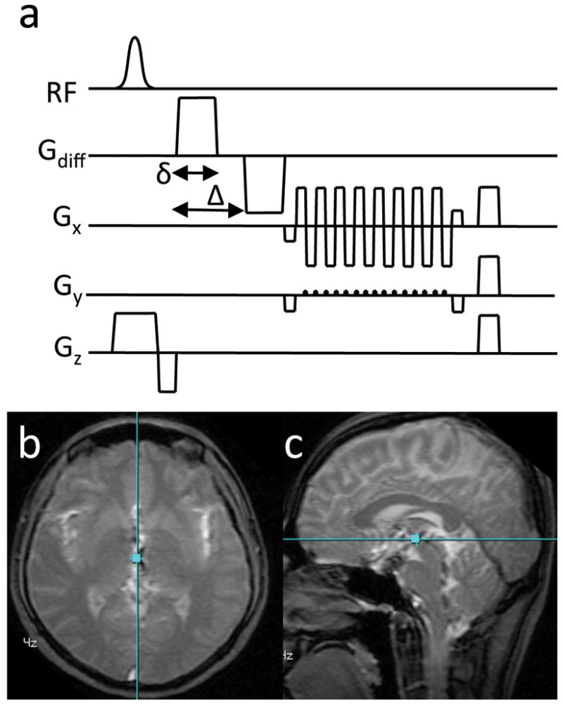
a) The DW-GRE pulse sequence depicting the bi-polar diffusion encoding gradients. b) The localizer image of the axial slice showing the relative position of the sagittal slice (blue line). c) The localizer image of the sagittal slice showing the relative position of the axial slice (blue line). The images (b, c) are from Subject 3.

Image Reconstruction

All post-processing was performed using software developed in-house in MATLAB (Natick, MA, USA). Data collected on the ramps of the EPI readout gradients were gridded to a Cartesian grid. Un-acquired phase-encode lines were recovered by POCS (18, 19). Finally, images were reconstructed by performing the 2D inverse FFT on the fully sampled Cartesian k-space data.

Estimating the Non-Rigid-Body Phase Maps

Figure 2 contains a summary of the algorithm used to estimate the non-rigid-body phase errors, Φ_non–rigid(r⃗, i), from the DW image phase, Φ(r⃗, i), and the b = 0 image phase, Φ_b0(r⃗). Essentially the terms Φ_rigid(r⃗, i) and Φ_ΔDW(r⃗) are estimated and Eq [9] is solved for Φ _non–rigid(r⃗, i).

Figure 2.

A diagram of the processing that was done to obtain the non-rigid-body phase maps (h), from the raw phase images of the diffusion weighted images (a). UW is the phase-unwrapping operator.

First, to remove most of the static phase, the unwrapped b = 0 image phase, Φ_b0(r⃗), was subtracted from the unwrapped DW image phase, Φ(r⃗, i), from each of the 250 time-points (20) (Fig 2a–d) to obtain an intermediate phase map, Φ _A(r⃗, i)(Fig 2e),

$${\mathrm{\Phi }}_A(\overrightarrow{r},i)=UW(\mathrm{\Phi }(\overrightarrow{r},i))-UW({\mathrm{\Phi }}_{b0}(\overrightarrow{r},i))$$ [10]

where UW is the phase unwrapping operator. Then, to remove the individual rigid-body phase terms from each of the 250 DW images, Eq [8] was fit to Φ_A(r⃗, i) over pixels lying within the brain to obtain the rigid-body phase map, Φ_rigid(r⃗, i) (Fig 2f). The rigid-body phase maps were then subtracted from Φ_A(r⃗, i) to obtain a second intermediate phase map, Φ_B (r⃗, i) (Fig 2g),

$${\mathrm{\Phi }}_B(\stackrel{\rightharpoonup }{r},i)={\mathrm{\Phi }}_A(\stackrel{\rightharpoonup }{r},i)-{\mathrm{\Phi }}_{\mathit{rigid}}(\stackrel{\rightharpoonup }{r},i).$$ [11]

Note that since the rigid-body phase, Φ_rigid(r⃗, i), and the b = 0 image phase, Φ_b0(r⃗), have been subtracted from the DW image phase, Φ(r⃗, i), that by Eq [9], Φ_B (r⃗, i) can be expressed as

$${\mathrm{\Phi }}_B(\stackrel{\rightharpoonup }{r},t)={\mathrm{\Phi }}_{\mathrm{\Delta }DW}(\stackrel{\rightharpoonup }{r})+{\mathrm{\Phi }}_{\mathit{non}-\mathit{rigid}}(\stackrel{\rightharpoonup }{r},t).$$ [12]

To isolate Φ_non–rigid(r⃗, i) from Φ_B (r⃗, i), it is assumed that the time average of Φ_non–rigid(r⃗, i) over all over the T acquired time points (recall that T=250 in the experiments) is 0,

$$\frac{1}{T}\sum _{i=1}^T{\mathrm{\Phi }}_{\mathit{non}-\mathit{rigid}}(\stackrel{\rightharpoonup }{r},i)=0,$$ [13]

which is equivalent to assuming that no net phase is accrued due to non-rigid-body motion over the entire exam. In other words, the non-rigid body motion was assumed to be periodic with no net displacement. This is similar to the approach taken in ref (14) except that here the phase wrap is addressed by the phase unwrapping step in Eq [10]. Then, since Φ_ΔDW (r⃗) (Fig 2h) does not depend on the TR number, i, by Eq [12] and Eq [13],

$$\frac{1}{T}\sum _{i=1}^T{\mathrm{\Phi }}_B(\stackrel{\rightharpoonup }{r},i)={\mathrm{\Phi }}_{\mathrm{\Delta }DW}(\stackrel{\rightharpoonup }{r})$$ [14]

and then finally the non-rigid-body phase, Φ_non–rigid(r⃗, i) (Fig. 2i), is obtained by combining Eq [12] and Eq [14],

$${\mathrm{\Phi }}_{\mathit{non}-\mathit{rigid}}(\stackrel{\rightharpoonup }{r},i)={\mathrm{\Phi }}_B(\stackrel{\rightharpoonup }{r},t)i-\frac{1}{T}\sum _{i=1}^T{\mathrm{\Phi }}_B(\stackrel{\rightharpoonup }{r},i).$$ [15]

Correlation Analysis

To assess the temporal correlation of the pulse-oximeter signal and the non-rigid-body phase maps, Φ_non–rigid(r⃗, i), Pearson’s linear correlation coefficient and corresponding p-values were computed between the pulse-oximeter signal and the time-varying signal in each pixel of Φ_non–rigid(r⃗, i) using MATLABs corr function. In the function, p-values were computed using the Student’s t-distribution. A pixel was determined to have a repeatable non-rigid-body phase if it had a p-value less than 0.05. The percentage of the p-values less than 0.05 across the entire image were computed for each of the six experiments and these percentages were averaged over subjects and experiments to give an overall impression of the level of repeatability observed. To account for different pulse travel duration between finger and brain, a delay was allowed between the pulse-oximeter signal and the time-dependent non-rigid-body phase in each voxel. The delay time that maximized the absolute correlation over the entire image of the axial slice with S/I diffusion encoding was used in the analysis.

Cardiac Binning

Raw pulse-oximeter waveforms with a sample spacing of 25 ms were obtained from the scanner host computer following each scan. Drift in the baseline and gain of the waveforms were corrected by applying a filter that forced the maximum of the pulse-oximeter signal to be 1 and the minimum to be 0 within a sliding window 3 seconds wide. Specifically, each point of the pulse-oximeter waveform was scaled by subtracting a local minimum and then dividing by a local maximum, where the local minimum and local maximum were the minimum and maximum of the signal within a 3 second wide rectangular window centered about the point. Peaks were detected according to 2 criteria: 1) the gradient of the signal is zero at that point and 2) the magnitude of the signal is greater than 0.5.

The time of the pulse-oximeter waveform was corrected for system and physiological delays by subtracting the delay found in the correlation analysis described above. An additional half bin width was added to the delay so that the peak of the pulse-oximeter waveform fell into the center of bin 1 (Fig 3). The image from each of the i TRs was assigned a normalized cardiac time, t_c(i), according to its relative position to the time of the peak occurring before it, t_p−(i), and the time of the peak occurring after it, t_p+(i), given by

Figure 3.

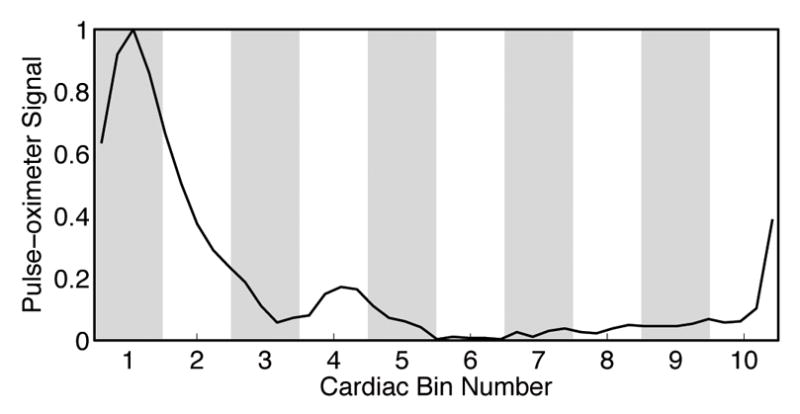
The relationship between the pulse-oximeter signal profile and the cardiac bins. Bin 1 corresponds to the systole, with the peak in the center of the bin. The pulse-oximeter signal from one heartbeat of Subject 2 is shown.

$$t_c(i)=\frac{t(i)-t_{p-}(i)}{t_{p+}(i)-t_{p-}(i)}$$ [16]

where t(i) is the time the image was acquired relative to the start of the scan. Both t_p−(i) and t_p+(i) are also measured relative to the start of the scan. Each of the i images was assigned to one of 10 cardiac bins, Bn, according to its normalized cardiac time, t_c(i),

$$B_n=\left\{i:\frac{n-1}{10}\le t_c(i)<\frac{n}{10}\right\}$$ [17]

where the bin number, n, ranged from 1 to 10. To ensure that the assumption of Eq [13] holds, the number of images in each cardiac bin was limited to the number of images in the bin with the fewest images.

Statistical Analysis

To quantify the beat-to-beat variability of the non-rigid-body phase within each of the 10 cardiac bins, the mean, m(r⃗, n), and standard deviation, σ(r⃗, n), of Φ_non–rigid(r⃗, i) was computed for the nth cardiac bin,

$$m(\stackrel{\rightharpoonup }{r},n)=\frac{1}{N_n}\sum _{i\in B_n}{\mathrm{\Phi }}_{\mathit{non}-\mathit{rigid}}(\stackrel{\rightharpoonup }{r},i),$$ [18]

and

$$\sigma (\stackrel{\rightharpoonup }{r},n)=\sqrt{\frac{1}{N_n}\sum _{i\in B_n}{[{\mathrm{\Phi }}_{\mathit{non}-\mathit{rigid}}(\stackrel{\rightharpoonup }{r},i)-m(\stackrel{\rightharpoonup }{r},n)]}^2},$$ [19]

where there are N_n images in n^th bin.

To assess whether the phases in the estimates of the m(r⃗, n) were significantly different from the zero-mean phase noise, a 2-tailed t-test was performed on each pixel. The t-statistic, τ, was computed according to,

$$\tau (\stackrel{\rightharpoonup }{r},n)=\frac{m(\stackrel{\rightharpoonup }{r},n)}{\sqrt{\frac{\sigma {(\stackrel{\rightharpoonup }{r},n)}^2}{N_n}+\frac{{\sigma }_{\mathit{phase}}^2}{T}}},$$ [20]

for each bin. Here, σ_phase is the standard deviation of the phase noise and T is the number of time-points measured total for the experiment. The number of degrees of freedom for the t-test was computed by,

$$v(\stackrel{\rightharpoonup }{r},n)=\frac{{\left(\frac{\sigma {(\stackrel{\rightharpoonup }{r},n)}^2}{N_n}+\frac{{\sigma }_{\mathit{phase}}^2}{T}\right)}^2}{\frac{\sigma {(\stackrel{\rightharpoonup }{r},n)}^4}{N_n^2(N_n-1)}+\frac{{\sigma }_{\mathit{phase}}^4}{T^2(T-1)}}.$$ [21]

Maps of the p-value, S(r⃗, n) were computed for each cardiac bin from the t-statistic, τ(r⃗, n), and the number of the degrees of freedom, υ(r⃗, n). The percentage of the pixels in S(r⃗, n) having p-values less than 0.05 were computed for each bin and also over all cardiac bins for an average value. The percentages were averaged over all subjects and experiments to give an overall impression of the level of repeatability observed. In pixels having having p-values less than 0.05 the statistical test shows that, at the 95 percent confidence level, those pixels demonstrate non-rigid-body phase that is repeatably different from the background noise from beat-to-beat.

Noise Quantification

To estimate the value of the parameter σ_phase that appears in Eq [20] and Eq [21], MRI was performed on a spherical agar phantom with the same MRI parameters as in the human scan described above. Because the phantom is assumed to have isotropic diffusion properties, only one axial slice of the phantom was scanned with the diffusion gradient oriented along the S/I direction. The SNR of the magnitude image was computed from the 250 time-resolved DW images (21). Then, to get an estimate of the lower bound of SNR, the minimum value of this SNR map was computed over the region of support of the phantom to get SNR_mag From this, the standard deviation of the phase image, σ_phase, in radians, was computed from the simple relationship (22),

$${\sigma }_{\mathit{phase}}=\frac{1}{{\mathit{SNR}}_{\mathit{mag}}}.$$ [22]

Since the phantom had different relaxation and diffusion parameters than human brain, this figure had to be adjusted by the ratio of the GRE signal equation.

Results

Noise Quantification

The standard deviation of the phase maps in the absence of physiologic noise, σ_phase, was estimated from the measurements in the agar phantom to be 0.043 rad. Note that the statistical parameters given by Eq [20] and Eq [21] are fairly robust to errors in the estimation of σ_phase since the sums in the denominators of each equation will be dominated by the larger σ (r⃗, n) term.

Volunteer Studies

Table 1 gives the percentage of pixels having a p-value less than 0.05 in the maps of temporal correlation coefficient of the pulse-oximeter signal to the non-rigid-body phase maps. With the exception of the A/P diffusion direction in the sagittal slice, all of the maps from all subjects have 75% or more pixels significantly correlated with the pulse-oximeter signal indicating a very high degree of correlation of the non-rigid-body phase with the cardiac cycle. The delay times and heart rates measured for each subject are also shown in the last 2 columns of Table 1. The maps of the correlation coefficient for all experiments in all subjects are shown in Figure 4. The correlation is strongest in the S/I direction, in agreement with the numerical data in Table 1. Note the varying patterns of positive and negative correlation with diffusion direction due to the differences in tissue motion along each axis.

Table 1.

The percentage of pixels having p-value < 0.05 in the Pearson’s correlation coefficient maps and the delay time between the pulse-oximeter signal and the image data that gave the maximum absolute correlation (second-to-last column). The heart rate for each subject is given in beats per minute in the last column.

Plane Diffusion Direction	Axial			Sagittal			avg	Delay, s	Heart rate, bpm
	S/I	L/R	A/P	S/I	L/R	A/P
Subject 1	95	92	87	81	86	52		0.16	71
Subject 2	97	95	94	86	91	56		0.08	56
Subject 3	96	87	91	78	84	40		0.13	72
Average	96	91	91	82	87	49	83		66

Figure 4.

Map of the Pearson’s Correlation Coefficient of the pulse-oximeter signal to the time-varying non-rigid-body phase in each pixel for all scans of all subjects. The spatial patterns of correlation are very similar for all 3 subjects in all cases accept for the sagittal slice with A/P diffusion direction.

Figure 5 shows the non-rigid-body phase maps, Φ_non–rigid(r⃗, i), from the S/I diffusion, axial slice in subject 1 for all time-points falling into cardiac bin 1 (Fig 5a), and into cardiac bin 7. It is visually apparent that the non-rigid-body phase maps are fairly similar within a bin. Note that in bin 1, which corresponds to the more dynamic period of systole, the non-rigid-body phase maps show more variation than those in bin 7 (Fig 5a), in which motion is less rapid.

Figure 5.

All of the non-rigid-body phase maps falling into cardiac bins 1 (a) and 7 (b) from subject 1. Note that the phase maps in each bin are very similar, demonstrating the repeatability of the non-linear phase patterns over the cardiac cycle. However, more variability is observed in bin 1 (a) than in bin 7 (b) reflecting the more rapid dynamics in systole compared with diastole. Also note that bin 1 (a) has a different colorbar than bin 7 (b).

A summary of the results from Subject 1 is shown in Figures 6, 7, and 8. From the non-rigid-body phase maps on the axial slice (Fig 6a) it is apparent that the S/I direction displays the greatest phase changes (Fig 6a, top row), followed by the L/R direction (Fig 6a, middle row), and then the A/P direction (Fig 6a, bottom row) with the weakest changes in the non-rigid-body phase maps. Also note that the greatest changes in the non-rigid-body phase maps in all three directions are associated with cardiac bin 1 (Fig 6, column 1), which corresponds to systole. The same general trends are apparent in the sagittal slices acquired in the same subject (Fig 6b). Fig. 6a and 6b also show the distinct motion of the brainstem and midbrain relative to the cerebrum and cerebellum. With the L/R encoding, one can also see the opposing direction of motion for the left and right hemisphere as shown by the positive and negative phase accrual, which is indicative of the lateral expansion during systole. Fig 7 shows that the standard deviation of the non-rigid-body phase tends to be higher in bin 1 corresponding to systole (Fig 7, first column) than in the later bins corresponding to diastole. However, despite the increased standard deviation during bin 1, most of the pixels over the brain display a significant non-rigid-body phase change in bin 1 (Figure 8, first column, red pixels).

Figure 6.

A comparison of the mean non-rigid-body phase maps from the axial (a) and sagittal (b) slices from subject 1. Note that cardiac bin 1 (corresponding to systole) is windowed differently from the other cardiac bins since the phase values are lower in the diastolic portion of the cardiac cycle.

Figure 7.

A comparison of the maps of the standard deviation non-rigid-body phase from the axial (a) and sagittal (b) slices from subject 1.

Figure 8.

A comparison of the p-value maps in all cardiac bins from the axial (a) and sagittal (b) slices from subject 1. Note that the pixels with p-values less than 0.05 are shown in red.

Table 2 shows the percentage of the pixels in the p-value maps S(r⃗, i) that had p-values of less than 0.05 on the t-test. In general, maps of S(r⃗, i) from bin 1 had more significant pixels than the average for all subjects, reflecting the greater overall non-rigid-body motion phase in the bin corresponding to systole. Comparing the numbers in table 2 to the p-value maps from subject 1 in Fig 8 the same trends can be observed. More pixels are significant in bin 1 in general than in the other bins, and more generally where the mean value of the non-rigid-body phase within a bin is higher, there are more significant pixels. Of course, this is due to the fact that the t-statistic in Eq [20] is proportional to the mean value of the non-rigid-body phase. These p-value maps show that the non-rigid-body phase is very repeatable from beat-to-beat over a large region of the brain.

Table 2.

The percent of the pixels in S(r⃗, n) that are significant (p < 0.05) averaged over all cardiac bins (all) and in the bin corresponding to systole (bin 1).

Plane Diffusion Direction	Axial						Sagittal						avg.
	S/I		L/R		A/P		S/I		L/R		A/P
-	all	bin 1	all	bin 1	all	bin 1	all	bin 1	all	bin 1	all	bin 1
Subject 1	74	88	75	80	72	45	72	79	73	78	32	38
Subject 2	80	95	74	92	68	84	47	64	60	79	40	40
Subject 3	70	88	66	76	61	82	65	79	50	62	19	14
avg. all	74		72		67		61		61		30		61
avg. bin 1		90		82		70		74		73		31	70

An abbreviated summary of the imaging results from subject 2 are given in Fig 9. Here the mean value of the non-rigid-body phase from bin 1 is given with corresponding standard deviation and p-value maps for each diffusion direction in the axial slice. The spatial patterns observed in these maps are very similar to those observed in subject one (Fig 6a, 7a, and 8a, first column). The larger non-rigid-body phase values observed in the images with S/I diffusion encoding compared with the other encoding directions is also consistent with results from subject one. Also apparent from the p-value maps (Fig 9, 3rd column) is the high repeatability of the non-rigid-body phase from beat-to-beat.

Figure 9.

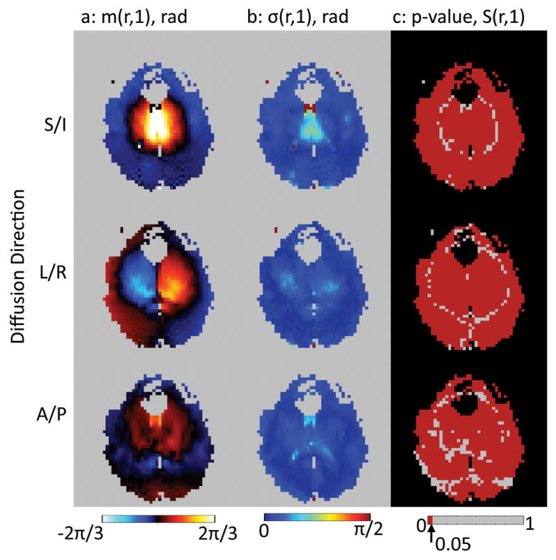
A comparison of the mean non-rigid-body phase maps (a), standard deviation of the non-rigid-body phase maps (b), and the p-value maps (c) from the cardiac bin with the greatest non-rigid-body phase, bin 1. Data from Subject 2 shown.

Figure 10 provides a comparison of the non-rigid-body phase in subjects 2 and 3 from the axial slice, for all three diffusion-encoding directions. This can be compared with Fig 6a which shows the corresponding images from subject 1. While the spatial and temporal patterns of the non-rigid-body phase are similar across all subjects there are differences. Some general patterns can be observed, however. First, the non-rigid-body phase in the S/I direction is the greatest. Second, the phases are at their greatest near systole (bin 1), then reduce in amplitude and reverse polarity as the tissue comes back to its resting position during diastole. Finally, regarding the non-rigid-body phase, there is no truly quiescent period. The phase appears to be changing throughout the cardiac cycle.

Figure 10.

Comparison of mean non-rigid-body phase in each cardiac bin in subjects 2–3. Note that cardiac bin 1 (corresponding to systole) is windowed differently from the other cardiac bins since the phase values are lower in the diastolic portion of the cardiac cycle.

Measurements of the non-rigid-body phase in an ROI (Fig 11b, red box) placed in the axial slice from subject 2 are presented in Fig 11a. The mean and standard deviation of the non-rigid-body phase within each bin are plotted (Fig 11, squares and errorbars) vs. the bin number. For reference a single cycle of the pulse oximeter is shown below in black. Also the mean of the non-rigid-body phase in the ROI is plotted vs. normalized cardiac time times 10 (to correspond to the bin numbers) for each individual image (Fig 11, small points). The key observation here is that the increased standard deviation in bin 1, for instance, appears to be due to rapid change of phase within the bin rather than actual physical variation in the phase from beat to beat.

Figure 11.

a) Plot of the mean value of the non-rigid-body phase and standard deviation of the non-rigid-body phase (solid lines, error bars) in an ROI in the axial scan (b) in subject 2. The ROI position is indicated in the b₀ image (b) by a red box. The mean values of the individual phase non-rigid-body phase maps are shown as the individual data points. The blue, green, and red lines correspond to the S/I, L/R, and A/P diffusion directions respectively. For reference one cycle of the pulse-oximeter waveform is shown in black at the bottom.

Discussion

The model for phase in DW-MRI developed here was used to isolate the phase due to non-rigid-body motion in the brain. The key observations in this work regarding this non-rigid-body phase are that it is:

1. greatest when diffusion-encoding is in the S/I, followed by L/R, then A/P with the lowest phase.

2. greater near the brainstem, midbrain, and pons.

3. highly correlated with pulse-oximeter waveforms

4. repeatable from beat-to-beat.

5. similar but not identical in spatial and temporal behavior across the healthy subjects observed.

Observations 1 and 2 are in line with previous work examining the motion of the brain (11, 12, 13, 14). Particularly the observation noted in the discussion of fig 9, i.e. that there is no truly quiescent period is in direct agreement with the observation in Ref (14) that the brain motion “appears to consist of a single displacement in systole followed by a slow return to the initial configuration in diastole”. This suggests that the non-rigid-motion cannot be dealt with in general by simple cardiac gating because the brain is always in motion. This problem will be even greater at higher b-values since, for example in the simplifying case of constant velocity, the motion-induced phase depends linearly on all three parameters that control the b-value, the gradient magnitude, gradient duration, and diffusion time Eq [5]. Cardiac gating can, at least, freeze the non-linear phase error and makes it predictable from beat-to-beat. Given the fact that during systole non-linear phase errors and hence corresponding k-space dispersion is largest, a proper delay that pushes the acquisition to a more quiescent period is advisable.

Observation 3 implies that cardiac monitoring with a pulse-oximeter (plethysmograph) can give sufficient fidelity to group the shots into the cardiac bins needed to do retrospective correction of the non-rigid-body phase. Furthermore, the correlation analysis performed here corrects for delays between the data acquisition and the pulse-oximeter waveforms due to physiology and hardware. Recent efforts to perform cardiac gating using the acquired data itself (23) suggest that even the pulse-oximeter apparatus may be done away with. This would make it much easier to bring retrospective non-rigid-body motion correction and hence multi-shot DW to routine practice.

Observation 4 supports the hypothesis that non-rigid-body motion in the brain is repeatable from beat to beat over many cardiac cycles. This provides a foundation for efforts such as those in Ref (10) to perform 3D phase navigation by measuring the non-rigid-body motion over multiple shots and grouping them together to form phase navigators for the non-rigid-body motion. Furthermore the observation that the standard deviation of the non-rigid-body phase is higher during systole supports the decision to exclude shots acquired during systole in previous works (10, 24), even with the grouping of shots in similar portions of the cardiac cycle to form non-rigid-body navigators (10). However, the results presented in Fig 11 suggest that with finer binning around systole, that these shots may perhaps be used.

In the three subjects examined, the patterns of correlation of the non-rigid-body phase with the pulse-oximeter signal (Fig 4) and the non-rigid-body phase as a function of cardiac bin were quite similar. However the differences are such that it would be difficult to derive a correction based on data from one individual and use it to correct data from others. This means that the non-rigid-body phase would have to be measured in each individual both in retrospective, navigator-based methods, as well as in more recently proposed prospective RF-based methods (25).

To keep the TR low and allow assessment of the non-rigid-body phase with a small temporal footprint, this study was done with a relatively low b-value (250s/mm²) compared to standard clinical practice. At higher b-values, the expected phase changes would increase (see Eqs [5] and [6], for instance), but the repeatability of the non-rigid-body phase should be the same since the underlying tissue motion is the same. One key difference, however, is that with higher b-values, the corresponding k-space dispersion is higher. This may cause errors with the partial-Fourier (POCS) method used in this study, due to the signal being dispersed outside of the sampled region (26). In this case the number of overscans would have to be increased, which in turn, would increase TE and ultimately reduce the time-resolution of the technique.

Conclusions

In this work, a phase model for DW-MRI of the brain was presented. In this model, static phase and dynamic phase were separated. Furthermore, in this model non-rigid-body motion-induced phases were assumed to be repeatable with the cardiac cycle from beat-to-beat. This assumption was tested in human volunteers and found to be valid to good approximation. Averaged across all subjects and diffusion directions investigated, the non-rigid-body phase in 83 percent of the brain territory investigated was significantly correlated to the pulse-oximeter waveform. In future efforts to improve 3D DW-MRI this assumption can be used to reduce the time spent collecting 3D phase navigators without sacrificing the ability to correct for non-rigid-body motion. The key benefit of reducing the navigation time is increased scan-time efficiency that can be used to increase spatial resolution, attain higher b-values, or acquire more encoding directions. This design flexibility afforded by this increased scan-time efficiency may ultimately bring high-resolution isotropic 3D DW-MRI of the whole brain closer to clinical reality.

References

- 1.Ordidge R, Helpern J, Qing Z, Knight R, Nagesh V. Correction of motional artifacts in diffusion-weighted MR images using navigator echoes. Magn Reson Imag. 1994;12:455–460. doi: 10.1016/0730-725x(94)92539-9. [DOI] [PubMed] [Google Scholar]
- 2.Anderson A, Gore J. Analysis and correction of motion artifacts in diffusion weighted imaging. Magn Reson Med. 1994;32:379–387. doi: 10.1002/mrm.1910320313. [DOI] [PubMed] [Google Scholar]
- 3.DeCrespigny A, Marks M, Enzmann D, Moseley M. Navigated diffusion imaging of normal and ischemic human brain. Magn Reson Med. 1995;33:720–728. doi: 10.1002/mrm.1910330518. [DOI] [PubMed] [Google Scholar]
- 4.Butts K, de Crespigny A, Pauly J, Moseley M. Diffusion-weighted interleaved echo-planar imaging with a pair of orthogonal navigator echoes. Magn Reson Med. 1996;35:763–770. doi: 10.1002/mrm.1910350518. [DOI] [PubMed] [Google Scholar]
- 5.Butts K, Pauly J, DeCrespigny A, Moseley M. Isotropic diffusion-weighted and spiral-navigated inter-leaved EPI for routine imaging of acute stroke. Magn Reson Med. 1997;38:741–749. doi: 10.1002/mrm.1910380510. [DOI] [PubMed] [Google Scholar]
- 6.Bammer R, Aksoy M, Liu C. Augmented generalized SENSE reconstruction to correct for rigid body motion. Magn Reson Med. 2007;57:90–102. doi: 10.1002/mrm.21106. [DOI] [PMC free article] [PubMed] [Google Scholar]
- 7.Miller K, Pauly J. Nonlinear phase correction for navigated diffusion imaging. Magn Reson Med. 2003;50:343–353. doi: 10.1002/mrm.10531. [DOI] [PubMed] [Google Scholar]
- 8.Liu C, Moseley M, Bammer R. Simultaneous phase correction and SENSE reconstruction for navigated multi-shot DWI with non-cartesian k-space sampling. Magn Reson Med. 2005;54:1412–1422. doi: 10.1002/mrm.20706. [DOI] [PubMed] [Google Scholar]
- 9.Atkinson D, Counsell S, Hajnal J, Batchelor P, Hill D, Larkman D. Nonlinear phase correction of navigated multi-coil diffusion images. Magn Reson Med. 2006;56:1135–1139. doi: 10.1002/mrm.21046. [DOI] [PubMed] [Google Scholar]
- 10.McNab J, Gallichan D, Miller K. 3D steady-state diffusion-weighted imaging with trajectory using radially batched internal navigator echoes (TURBINE) Magn Reson Med. 2010;63:235–242. doi: 10.1002/mrm.22183. [DOI] [PubMed] [Google Scholar]
- 11.Feinberg D, Mark A. Human brain motion and cerebrospinal fluid circulation demonstrated with MR velocity imaging. Radiology. 1987;163:793. doi: 10.1148/radiology.163.3.3575734. [DOI] [PubMed] [Google Scholar]
- 12.Greitz D, Wirestam R, Franck A, Nordell B, Thomsen C, Ståhlberg F. Pulsatile brain movement and associated hydrodynamics studied by magnetic resonance phase imaging. Neuroradiology. 1992;34:370–380. doi: 10.1007/BF00596493. [DOI] [PubMed] [Google Scholar]
- 13.Enzmann D, Pelc N. Brain motion: measurement with phase-contrast MR imaging. Radiology. 1992;185:653. doi: 10.1148/radiology.185.3.1438741. [DOI] [PubMed] [Google Scholar]
- 14.Poncelet B, Wedeen V, Weisskoff R, Cohen M. Brain parenchyma motion: measurement with cine echo-planar MR imaging. Radiology. 1992;185:645. doi: 10.1148/radiology.185.3.1438740. [DOI] [PubMed] [Google Scholar]
- 15.Bernstein M, King K, Zhou X. Handbook of MRI Pulse Sequences. Elsevier Academic Press; Burlington, MA, USA: 2004. [Google Scholar]
- 16.Hiltunen J, Hari R, Jousmäki V, Müller K, Sepponen R, Joensuu R. Quantification of mechanical vibration during diffusion tensor imaging at 3T. Neuroimage. 2006;32:93–103. doi: 10.1016/j.neuroimage.2006.03.004. [DOI] [PubMed] [Google Scholar]
- 17.Gallichan D, Scholz J, Bartsch A, Behrens T, Robson M, Miller K. Addressing a systematic vibration artifact in diffusion-weighted MRI. Hum Brain Mapp. 2010;31:193–202. doi: 10.1002/hbm.20856. [DOI] [PMC free article] [PubMed] [Google Scholar]
- 18.Cuppen J, van Est A. Reducing mr imaging time by one-sided reconstruction. Magn Reson Imag. 1987;5:526–527. [Google Scholar]
- 19.Haacke E, Lindskogj E, Lin W. A fast, iterative, partial-fourier technique capable of local phase recovery. J Magn Reson. 1991;92:126–145. [Google Scholar]
- 20.Jenkinson M. Fast, automated, n-dimensional phase-unwrapping algorithm. Magn Reson Med. 2003;49:193–197. doi: 10.1002/mrm.10354. [DOI] [PubMed] [Google Scholar]
- 21.Reeder S, Wintersperger B, Dietrich O, Lanz T, Greiser A, Reiser M, Glazer G, Schoenberg S. Practical approaches to the evaluation of signal-to-noise ratio performance with parallel imaging: Application with cardiac imaging and a 32-channel cardiac coil. Magn Reson Med. 2005;54:748–754. doi: 10.1002/mrm.20636. [DOI] [PubMed] [Google Scholar]
- 22.Haake E, Brown R, Thompson M, Venkatesan R. Magnetic Resonance Imaging. Physical Principles and Sequence Design. John Wiley & Sons Inc; New York, NY, USA: 1999. [Google Scholar]
- 23.Curcic J, Buehrer M, Boesiger P, Kozerke S. Prospective self-gating for simultaneous compensation of cardiac and respiratory motion. 16th Annual Proceedings of the ISMRM; Toronto, Ontario, Canada. 2008. p. 203. [DOI] [PubMed] [Google Scholar]
- 24.Jung Y, Samsonov A, Block W, Lazar M, Lu A, Liu J, Alexander A. 3D diffusion tensor MRI with isotropic resolution using a steady-state radial acquisition. J Magn Reson Imag. 2009;29:1175–1184. doi: 10.1002/jmri.21663. [DOI] [PMC free article] [PubMed] [Google Scholar]
- 25.Nunes R, Malik S, Hajnal J. Prospective correction of spatially non-linear phase patterns for diffusion-weighted fse imaging using tailored rf excitation pulses. 19th Annual Proceedings of the ISMRM; Montreal, Quebec, Canada. 2011. p. 172. [Google Scholar]
- 26.Storey P, Frigo F, Hinks R, Mock B, Collick B, Baker N, Marmurek J, Graham S. Partial k-space reconstruction in single-shot diffusion-weighted echo-planar imaging. Magn Reson Med. 2007;57:614–619. doi: 10.1002/mrm.21132. [DOI] [PubMed] [Google Scholar]