

Abstract
The fast Fourier transformation has been the gold standard for transforming data from time to frequency domain in many spectroscopic methods, including NMR. While reliable, it has as a drawback that it requires a grid of uniformly sampled data points. This needs very long measuring times for sampling in multidimensional experiments in all indirect dimensions uniformly and even does not allow reaching optimal evolution times that would match the resolution power of modern high-field instruments. Thus, many alternative sampling and transformation schemes have been proposed. Their common challenges are the suppression of the artifacts due to the non-uniformity of the sampling schedules, the preservation of the relative signal amplitudes, and the computing time needed for spectra reconstruction. Here we present a fast implementation of the Iterative Soft Thresholding approach that can reconstruct high-resolution non-uniformly sampled NMR data up to four dimensions within a few hours and make routine reconstruction of high-resolution NUS 3D and 4D spectra convenient. We include a graphical user interface for generating sampling schedules with the Poisson-Gap method and an estimation of optimal evolution times based on molecular properties. The performance of the approach is demonstrated with the reconstruction of non-uniformly sampled medium and high-resolution 3D and 4D protein spectra acquired with sampling densities as low as 0.8%. The method presented here facilitates acquisition, reconstruction and use of multidimensional NMR spectra at otherwise unreachable spectral resolution in indirect dimensions.
Keywords: nuclear magnetic resonance, sparse sampling, spectra reconstruction, iterative soft thresholding, compressed sensing, maximum entropy reconstruction, FM reconstruction
Introduction
The high magnetic field strengths of modern NMR spectrometers have increased the spectral resolution available for studies of complex biological macromolecules, such as proteins and nucleic acids. Common procedures for resonance assignment and structure determination employ multidimensional experiments, which involve evolution periods in several indirect dimensions. These have traditionally been sampled by proceeding through linear equidistant increments of the evolution times. Ideally, one wants to sample each indirect dimension to about 1.2 times the value of the relaxation time, T2, for the evolving coherences (Rovnyak et al. 2004b). Unfortunately, the time needed for uniform sampling through all increments in 3D and 4D spectra allows only to reach a fraction of the optimal evolution times (Rovnyak et al. 2004b) and the resolving power of modern instrument is only marginally utilized in the indirect dimensions. To reach the optimal range of evolution times in a reasonable overall measuring time can only be achieved with non-uniform sampling (NUS) as pointed out before (Rovnyak et al. 2004b). This requires however spectral reconstruction methods different from the Fast Fourier Transformation (FFT). Obviously, the quality of the resulting spectra depends crucially on the sampling schedules and the reconstruction methods, which has become an important field of recent research. Numerous sampling schedules have been proposed, such as exponentially weighted (Barna et al. 1987) or uniformly random sampling (Mobli et al. 2006; Kazimierczuk et al. 2008; Rovnyak et al. 2004a). Different approaches of radial or concentric sampling have also been proposed (Kupce and Freeman 2003; Coggins and Zhou 2008). Recently, it was suggested to select the gaps of skipped sampling grid points according to a Poisson distribution (Hyberts et al. 2010; Hyberts et al. 2011) or arranging sampling points picked using Poisson discs (Kazimierczuk et al. 2008).
Several methods have been proposed for reconstructing sparsely sample multidimensional NMR data. The initial approaches used different versions of Maximum Entropy principles (Barna et al. 1987; Hoch 1989) but a variety of other methods have also been developed since. The power of NUS is getting increasingly recognized in general, and methods for reconstructing such data have now collectively been called Compressed Sensing (CS). This term has been introduced and popularized by Donoho who provided a detailed theoretical basis for the validity of reconstructing frequency-domain data from sparse (NUS) data (Donoho 2006). A similar general analysis of stability and robustness of extending incomplete data has been provided by Candes and coworkers (Candes et al. 2006).
Examples of methods for reconstructing NUS NMR data, and which would fall under the term compressed sensing include the filter diagonalization (FDM) method (Chen et al. 2004; Mandelshtam et al. 1998), various applications of the CLEAN procedure (Coggins and Zhou 2008; Högbom 1974; Kupce and Freeman 2005; Wen et al. 2011), or the multidimensional decomposition method (MDD)(Tugarinov et al. 2005; Hiller et al. 2009; Denk et al. 1986). Recently, we have developed the Forward Maximum entropy (FM) method that reconstructs incomplete time domain data by an iterative approach using a conjugate gradient minimization of a target function (Hyberts et al. 2007). The target function is a norm of the frequency spectrum, such as the negative entropy, the sum of the absolute values of the frequency data points or others. The performance of the routine was improved when combined with a distillation module (Hyberts et al. 2009), which is also related to the CLEAN procedure (Högbom 1974). Using this reconstruction method it was shown that sensitivity can be gained for a given total measurement time when compared to uniform sampling(Hyberts et al. 2010). Thus, the software developed for the FM approach provides excellent reconstructions of spectra non-uniformly sampled in one or two indirect dimensions (Hyberts et al. 2011; Hyberts et al. 2009) but is computationally expensive for 3D and 4D NMR spectra. In particular, it is not efficient enough for routine reconstruction of high-resolution NUS 4D NMR spectra. Another recent procedure of compressed sensing has been described by Nietlispach and coworkers (Holland et al. 2011) who perform a minimization of the l1 norm of spectra to reconstruct NUS time domain data, which is mathematically equivalent to IST as shown (Stern et al. 2007) and is related to previous approaches (Hyberts et al. 2007; Lustig et al. 2007). They show that excellent reconstruction of 2D 1H-15N and 3D HNCA and HNCOCA experiments can be obtained. A related variant of compressed sensing was shown recently using an iterative re-weighted least squares approach, which is closely related to the procedures described here (Kazimierczuk and Orekhov 2011). The authors also showed excellent quality reconstructions of 2D HSQC and 2D NOESY spectra. Overall, there are several viable techniques for reconstructing NUS 2D and 3D NMR experiments. Among these, gradient optimization approaches tend to be slow and make reconstruction of 4D NUS time consuming. The MDD approach is fast but needs evaluation with regard to sensitivity and complete recovery of peaks (Hiller et al. 2009). The MDD package includes an IST option, which is also included in the recent Bruker TopSpin software. The SIFT approach is another technique for reconstruction of NUS spectra (Matsuki et al. 2009). Here knowledge about spectral regions that do not contain signals is used, and frequency-domain data points are set to zero in reconstruction cycles prior to inverse FFT to supplement time domain data. Kozminski and coworkers have developed a procedure termed SSA (Signal Separation Algorithm) (Stanek and Kozminski 2010; Stanek et al. 2011), which is a hybrid approach that combines the concepts of CLEAN (Högbom 1974) and manual artifact removal (Kazimierczuk et al. 2007).
Thus, searching for simple faster and reliable reconstruction methods for NUS NMR spectra we embarked on implementing the iterative soft thresholding (IST) approach. The use of iterative thresholding has been proposed previously for extracting unknown functions from noisy data (Donoho 1995). It has been used for reconstruction of sparse data in MRI (Suzuki and Toriwaki 1991) and other imaging methods, such as magnetic force microscopy (Ting et al. 2009). In high-resolution NMR, IST has been discussed for extending truncated uniformly sampled NMR data in the time domain (Stern et al. 2007). To our knowledge, the use of IST for reconstructing sparse NMR data has first been proposed by Drori who used a wavelet transform rather than the more commonly used FFT (Drori 2007).
Here we describe a simple adaptation of IST that can reconstruct NUS NMR spectra up to four dimensions very fast. The program developed follows the IST principle, such as outlined by Drori who employs wavelet transformations (Drori 2007). Our approach only uses the FFT and its inverse, which makes the reconstruction very fast compared to FM. The implementation described here largely eliminates the artifacts arising from the non-uniform sampling schedule. We provide a graphical user interface (GUI) for creating schedules with the Poisson-Gap sampling method up to three indirect dimensions. We demonstrate that processing based on this IST principle can efficiently and faithfully reconstruct up to 4D NUS NMR spectra where up to three indirect dimensions are sampled non-uniformly. Here we use the Poisson-Gap approach to select optimal sampling schedules (Hyberts et al. 2010; Hyberts et al. 2011). We show applications to a 15N-dispersed 3D HSQC-NOESY experiment and two four-dimensional methyl-methyl HC-NOESY-CH spectra on ILV-labeled samples with sampling densities of around 6%, 14.5% and below 0.8%. The simplicity of the algorithm currently allows reconstruction of these high-resolution 4D HC-NOESY-HC experiments within a few hours on a 128 CPU cluster. On a 25% sparse 1D time domain signal, the IST implementation described here is a factor of 534 faster than FM when using the same 3 GHz 32 Intel Xeon computer.
Materials and Methods
Protein Samples Used
A 15N labeled sample was prepared for the nuclear egress protein M50. This protein from mouse cytomegalo virus is critical for the movement of newly encapsidated viral particles from the nucleus to the cytoplasm. The molecular mass is 19.4 kDa. The sample concentration was 0.18 mM, which is the maximum concentration we can achieve due to solubility problems. Experiments were performed at 18°C since the protein is unstable at higher temperatures.
To obtain methyl-methyl NOEs in 4D NOESY spectra a complex of the MED25 component of the human Mediator with the transactivation domain (TAD) of the Herpes simplex transcriptional activator VP16 with a total molecular mass of 28 kDa was prepared. Both proteins were perdeuterated but 13C/1H labeled at the ILV methyl groups (Tugarinov and Kay 2004). Procedures of sample preparation have been described (Milbradt et al. 2011). A 1:1 ratio of VP16-TAD and MED25 was used to from a complex with a final concentration of 1 mM.
For recording an ultra-high resolution 4D methyl-methyl NOESY a 0.9 mM solution of a 10 kDa construct of protein G containing the B1 domain was prepared as described previously (Gronenborn et al. 1991; Zhou et al. 2001). The protein was perdeuterated but 13C/1H labeled at the ILV methyl groups (Tugarinov and Kay 2004).
NMR experiments
The 3D 15N dispersed NOESY experiment on the M50 protein was performed on a Bruker Avance 800 instrument at 298K. A total of 48 scans were recorded per increment. For the measurements the sweep width in the direct dimension was 11160.714 Hz, which was reduced to the HN area (11.0ppm – 5.5ppm) of 4403.250 Hz for the reconstruction. The sweep width in the indirect proton dimension was 9606.148 Hz ( 9.61 kHz), which was sampled in 400 increments of 0.104 ms and a maximum evolution time t-max of 41.62 ms. The sweep width in the indirect nitrogen dimension was 2000.000 Hz, which was sampled in 100 increments of 0.5ms and a maximum evolution time t-max of 50.00 ms. A total of 2400 increments out of the 40,000 point indirect Nyquist grid were measured resulting in a 6% sampling density.
The 4D methyl-methyl HMQC NOESY experiment on the MED25/VP16 complex was recorded on a Bruker Avance 750 instrument at 298K with the procedures described in (Hiller et al. 2009). The sampling schedule for the experiment on MED25/VP16 was generated with the MDD toolkit (Hiller et al. 2009). The sampling density was 14.5 %, with a maximum evolution time in the indirect dimensions of 17 ms in 1Hnoe, 13 ms in 13Cnoe, and 29 ms in 13Cdir. The numbers of complex indirect points in the Nyquist grid were 28 for 1Hnoe, 44 for 13Cnoe, and 96 for 13Cdir. The NOE mixing time was 150 ms. Spectral widths of the indirect dimensions were 1650 Hz in 1Hnoe, 3300 Hz in 13Cnoe and 13Cdir. The direct proton dimension was acquired for 77 ms with a spectral width of 10000 Hz. Four scans were recorded for each FID.
The 4D methyl-methyl HMQC NOESY experiment on GB1was recorded on a Bruker Avance 500 instrument at 303K using a methyl TROSY pulse sequence (Tugarinov et al. 2003)(Hiller et al. 2009). The schedule for the 4D methyl-methyl NOESY experiment on GB1 was generated with the Poisson Gap sampling GUI described below. The sampling density was 0.8 % with maximum evolution times in the indirect dimensions of 118 ms in 1Hnoe, 118.4 ms in 13Cnoe, and 118.8 ms in 13Cdir. The numbers of complex indirect points in the Nyquist grid were 60 for 1Hnoe, 150 for 13Cnoe, and 150 for 13Cdir. The NOESY mixing time was 120 ms. Spectral widths of the indirect dimensions were 500.1 Hz in 1Hnoe, 1257.6 Hz in 13Cnoe and 13Cdir. The direct proton dimension was acquired for 154 ms with a spectral width of 6666.7 Hz. Four scans were recorded for each FID.
Computation
The IST program was written in the C programming language and was implemented to run on a multiple cpu farm in parallel mode where the indirect data associated with each directly sampled data point are sent to one processor. We use a farm of 32 Intel Xeon computers each containing four 3 GHz cores operating at 64 bit. Processing times are indicated for the spectra shown below. The FM reconstructions were performed on a ServMax Tesla GPU HPC, which contains a 4-Core 3 GHz cpu with four Nvidia CUDA 240-Core cards. The Graphical User Interface (GUI) was written with GTK+, a cross-platform widget toolkit.
Results
IST reconstruction procedure
The procedure of the IST implementation is simple and is illustrated in Fig. 1. For demonstration we use a synthetic time domain data set containing two signals of different intensity, and no noise is added. To simulate sparse sampling, 75% of the data points (96 of 128) are set to zero using the Poisson-Gap sampling method (Hyberts et al. 2010; Hyberts et al. 2011). These sparse data are Fourier transformed with FFT. The frequency spectrum contains noise-like artifacts, which are, however, caused by the non-uniform sampling schedule. As the synthetic spectrum doesn’t contain noise, the artifacts are unrelated to ‘real’ noise. The PSF related artifacts due to non-uniform sampling are directly correlated with the height of the peaks. After the first FFT of the NUS time-domain data the tallest signal in the frequency domain data is identified, and a threshold slightly below its maximum is selected. In Fig. 1 this threshold is set at a height of 0.75 of the tallest peak (indicated with the dashed line). All data above this threshold value are moved to a secondary spectrum (right), which previously has been initialized with zeros at all frequency points. The residual spectrum, with the tallest signals truncated, is now converted back to a time-domain data set by inverse Fourier transformation. In this second-generation time domain data set, grid points not experimentally measured are again set to zero. At this point, one cycle is completed. In the second iteration the sparse time-domain data containing reduced tall peaks are again Fourier transformed, a new threshold is established, and the data above this threshold are removed and added to the secondary spectrum. The truncated spectrum is again converted to the time domain with inverse Fourier transformation. This procedure is iterated until the residual is nearly empty or below a user-defined threshold (see bottom left trace in Fig. 1). Here, 100 iterations eliminated the artifacts from NUS beyond detection in this simulated data set. For practical applications in spectra with noise and a high dynamic range we find that it beneficial to use small decreases of the threshold, such as 0.98. However, it seems possible to start with larger steps and to dynamically decrease the step sizes when approaching the noise. This could further accelerate the reconstruction process dramatically but has not been explored here.
Figure 1.
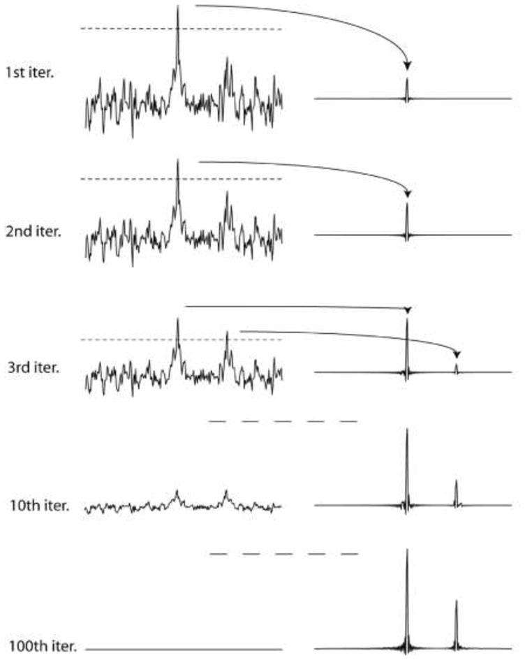
Illustration of the IST procedure. A synthetic time domain signal containing a large and a small resonance is sampled with a non-uniform Poisson-Gap sampling schedule (32 of 128 time-domain data points; 25% density). The line width was chosen so that 128 points correspond to T2. Time domain data were doubled with zero filling, and no apodization was applied prior to FFT, which is manifested in the sinc wiggles at the bases of the resonances. The top parts of the largest signals above a threshold are removed and stored in another file. The truncated spectrum is converted into a second-generation time domain signal by FFT-1, the points where the sampling schedule had zeros initially are set to zero again after the inverse Fourier transform, and the procedure is iterated. As all PSF-related artifacts caused by NUS come from the missing data points the final spectrum contains essentially no such artifacts.
The simulations in Fig. 2 explore the performance of IST in a synthetic spectrum of high dynamic range in the presence of noise. We consider three signals with relative heights of 50:2:1 and add random Gaussian noise with peak noise of 0.5. This resembles the situation of a strong NOESY diagonal peak and two weak cross peaks. The time domain consists of 1024 points on the Nyquist grid. The Fourier transform of the full time domain is shown at the top next to the transformation of the synthetic spectrum without noise where the relative peak intensities are indicated. We compare this with a time domain signal that has four times more scans per increment and the noise is lower by a factor of two. However, we sample only one quarter of the points (256 of 1024) using the Poisson Gap sampling method. Thus, both hypothetical experiments would require the same total measurement time. We apply the IST procedure to the NUS data set with a threshold of 98%. The first IST iteration exhibits strong artifacts from the NUS schedule primarily due to the strongest peak, and only the strongest peak appears in the first-iteration reconstructed spectrum. The artifacts gradually decrease during the iterations. While the strongest peak starts to be recovered quickly it takes more than 100 iterations to start recovering the weak peaks. At 500 iterations the residual is almost completely depleted and the reconstructed spectrum on the right represents the initial intensity distribution rather well. The noise in the reconstruction is less than half of that in the reference spectrum at the top, which supports the notion that the signal-to-noise ration can be significantly improved by NUS when the gain in measurement time is used to record more scans per increment (Hyberts et al. 2010). The relative intensities of the peaks are shown in Fig. 2B in dependence of the number of iterations. Note the strongest peak has been scaled by a factor of 10. The relative intensities of the two weak peaks are not exactly the same as in the noiseless reference spectrum at the top. The middle peak, which should have a relative intensity of 2 is slightly weaker. This is likely due to the random nature of the noise, which may add to the weaker peak or subtract from the stronger signal. This is consistent with the relative peak intensities in the reference spectrum with noise on top of Fig. 2A.
Figure 2.

Fidelity of peak reconstruction and termination criteria. (A) A synthetic spectrum was generated consistent of three Lorentzian lines with relative intensities 50:2:1 to resemble a situation of a NOESY spectrum with a strong diagonal and two small cross peaks. Random Gaussian noise was added with peaks noise of 0.5 relative intensity. The time domain signal consists of 1024 points. The line widths are set so that 1024 points correspond to T2. A regular FFT was applied to this simulated time-domain signal with and without noise to yield the references displayed on top. To simulate NUS, 256 of 1024 data points were selected using the Poisson-Gap sampling method (Hyberts et al. 2010), and the noise was scaled down by a factor of two to simulate equal overall measuring times of the NUS compared to the US data. The spectrum was reconstructed using IST and a threshold of 99.5%. Thus, the first iteration reconstruction contains the top of the strong signal at a relative peak height of 0.0025 (0.5% of 50). Various stages of the iteration are displayed with the residual on the left and the reconstructed spectrum on the right. The weaker signals appear only at around 150 iterations. (B) Heights of the three signals during the course of reconstruction. For display the strong signal was scaled by a factor of 10. The final relative intensities of the tallest and the smallest signal are approximately 50:1 as expected but signal 2 is smaller, which can be attributed to the stochastic effect of the noise. We terminate iterations when the residual is zero or below a user defined threshold. (C) The L2 norm (spectrum L2; square root of power) of the reconstructed spectrum increases during the iterations until the residual is nearly depleted. The residual L2 decreases almost linearly on a logarithmic scale and so does the increase of the reconstructed spectrum. The iteration can be terminates when the residual L2 drops below a user-defined value.
To establish termination criteria we plot in Fig. 2C the evolution during the iterations of the l2 norms (square root of power) for different spectral properties. The l2 norm for the residual is in cyan, for the reconstructed spectrum is in magenta, and for the increase of l2 (Δl2) of the reconstructed spectrum is in black. We terminate iterating when the residual is exhausted and no significant data are transferred to the reconstructed spectrum (see Figure 2A and 2C). This is done when the l2 norm of the residual is less than a user-defined value, such as ter =0.0001. Thus, the user has to define only two parameters, the step size of the iteration and the termination parameter.
The IST reconstruction outlined here is very fast and more efficient than the previously developed FM reconstruction (Hyberts et al. 2009). For the synthetic 1D spectrum used in Fig. 2, it is about 534 times faster. With n being the length of the Nyquist grid, IST has the advantage that the reconstruction scales in proportion to ndim × log(n) rather than n(dim+1) as in the FM approach. This is because IST utilizes only the FFT routine, and no matrix multiplication, as needed in the FM reconstruction. Hence, the IST reconstruction will always be faster than that of reconstruction routines that use matrix multiplications.
Graphical User Interface for Poisson Gap sampling
The IST approach is best utilized with an optimized NUS schedule. We have previously described the benefits of one-dimensional Poisson Gap sampling with sinusoidal weighting, as well as of a woven approach to generate a sampling schedule for two indirect dimensions(Hyberts et al. 2010; Hyberts et al. 2011). Here we extend the woven technique to three indirect dimensions, by stacking woven planes together. This is analogous to a set of woven panels put alternatively into a wooden box, such that the first woven plane is put at the bottom of the box. The second is then standing on the first plane and against one of the sides of the box; the third plane then standing on the first plane but against an orthogonal side of the box relative to the second plane. The fourth plane stands adjacent to the third, the fifth adjacent to the second, and the sixth is laying on the bottom on top of the first plane. As the woven planes have the width of one increment, the stacking in this way would cause the planes gradually sticking out of the top and sides of the Nyquist box. Hence, the areas of the planes are pre-adjusted to the area they will cover.
To conveniently create sampling schedules for up to three indirect dimensions we have developed a graphical user interface (GUI) shown in Figure 3. This allows accessing two back-end programs. On the one hand, it initializes creation of a Poisson-Gap sampling schedule(Hyberts et al. 2010) with a user defined sampling density. Setting a tolerance allows small deviations from the requested sampling density, which typically result as a consequence of the algorithm used to create the schedule. The user can set a seed number needed to initiate a Unix random number generator. On the other hand, the GUI guides the user to setting optimal maximum numbers of increments in the indirect dimensions, defining an optimal Nyquist grid, such as xN, yN and zN for a 4D experiment. This was guided by the idea that one optimally should sample indirect dimensions out to 1.2 × T2, where T2 is the relaxation time of the active coherence. Thus, providing the molecular weight, the temperature and the type of coherence, the program calculates approximate correlation times based on the well-known Stokes-Einstein formula . Here, rH is the effective hydrodynamic ration of the protein and is estimated from the molecular weight and assuming the protein is a perfect sphere. The user can override the calculated value if τc has been measured experimentally. The correlation time can also be estimated as measured correlation times fall roughly within the range 0.3xMW < τc < 0.9xMW when τc is in units of ns and MW is in kDa (Wagner 1997). Relaxation times of coherences active during the indirect dimensions are calculated with a C adaptation of the program COAST (Rovnyak et al. 2004b). The original COAST program is available at http://gwagner.med.harvard.edu. It calculates relaxation times based on well-known relations for 1H-15N pairs without (Peng and Wagner 1992) and with TROSY selection (Pervushin et al. 1997) and described in textbooks (Cavanagh et al. 2007). However, the values calculated should only be considered very rough estimates for guiding the choice of maximum evolution times and should not be misinterpreted as precise predictions of experimental transverse relaxation times. The estimated relaxation times can then be transferred manually to the boxes for the indirect dimensions. The factor next to the boxes defines then how far out to sample in units of the estimated T2. A factor of 1.2 would set the maximum evolution time to 1.2 × T2 of the respective coherence but any other factor can be used. Executing the program creates a sampling schedule that is visualized in the right-hand side of the GUI. The GUI also lists the total number of sampling points so that the user can estimate the total measuring time. The sweep-width may be entered in Hz, or ppm. In the latter case, the sweep-width in Hz is calculated via the spectrometer frequency and the nucleus in question.
Figure 3.

Screen shot of the graphical user interface (GUI) for generating Poisson-gap sampling schedules for up to three indirect dimensions and estimating relaxation properties of coherences. To estimate a maximum evolution time corresponding to T2 the total length of the Nyquist grid axis (np) is calculated as sweep width in Hz times T2. The Nyquist grid can be made longer or shorter be multiplying with a factor. The factor should be 1.2 in order to reach a maximum evolution time of 1.2 T2. The sweep-width may be entered in Hz, or ppm. In the latter case, the sweep-width in Hz is calculated via the spectrometer frequency and the nucleus in question. The sparsity of the sampling schedule can be selected with the button labeled “Sampling density”. It requires a tolerance because the Poisson Gap sampling method may create a schedule that does not exactly select the match the requested sparsity. Approximate values for the transverse relaxation times T2 can be estimated with the panel on top for various coherences typically used in triple resonance experiments. These rough estimates are based on correlation times estimated with the Stokes-Einstein formula and common equations for relaxation times as listed in (Peng and Wagner 1992; Peng and Wagner 1994; Wagner 1993). To our knowledge, relaxation rates for deuterated alpha carbons are not well understood and estimates made here use only proton-deuterium dipole-dipole relaxation have to be used with caution.
The sinusoidal weight can be set either as 1 or as 2 where the former value is used when denser sampling os both at the beginning and the end of the evolution time and uses one full half of the sine period to bias the lengths of the gaps in the Poisson-Gap sampling procedure. If a value of 2 is selected, only one quarter of the sine period is used leading to dense sampling at the beginning and long gaps at the end of the evolution time. As typically an apodization is applied that scales down the measured values at the end of the evolution time, the value 2 is the default option.
The sampling is finally determined by the seed value and the sampling density parameter, the latter entered as percentage. Note that the sampling density refers to overall multidimensional sampling density, not as a percentage axis wise.
The sequence of sampling points can be generated according to increasing time or in random order. If the latter is chosen sampling points are chosen all over, and at any time a NUS spectrum is present starting from zero sampling density and reaching the set sampling density at the end of the experiment, such as 3% in the example shown in Fig. 3.
Application to experimental spectra
To compare the performance of IST and FM reconstruction we recorded a 3D 15N dispersed NOESY on a 0.18 mM sample of the M50 protein, a component of the nuclear egress complex of mouse cytomegalo virus (Figure 4). In total, 2400 of 40,000 (6%) indirect data points were sampled and selected with the Poisson Gap sampling method. For comparison, the spectra were reconstructed with the FM and IST methods. As can be seen in the figure the reconstructed spectra are nearly identical. However, the IST reconstruction is orders of magnitudes faster (see caption to Figure 4).
Figure 4.

Comparison of FM and IST reconstruction of a 3D 15N dispersed NOESY recorded on a 0.8 mM sample of the M50 protein, a component of the mouse cytomegalovirus egress complex. The spectrum was recorded on a Bruker Avance 800 spectrometer at 298K. Data were sampled at 6% (2400 points) of a 400x100 (HxN) indirect Nyquist grid, selected with Poisson Gap sampling (Fig. 3). The representative plane compared is almost identical between FM and IST reconstruction. However, the FM reconstruction (500 iterations) took 1.5 days of parallel processing on a Cuda computer using 4 Nvidia GPU cards, whereas the IST reconstruction was completed within 4 hrs 45 min on a single cpu, and in just 3 minutes on a 128 cpu cluster.
To test IST on 4D spectra we reconstructed a NUS 4D HC-NOESY-HC spectrum of an ILV-labeled 28 kDa MED25/VP16 protein complex (Milbradt et al. 2011). The spectrum had been sampled with 14.5% sparsity. In Figure 5 we compare a representative plane reconstructed with straight FFT (left), FM (middle) and IST (right). When using straight FFT basically only the diagonal peak and the cross peak to the other methyl of the same residue (L486) can be seen while most of the spectrum of interest is obscured with artifacts due to NUS, and straight FFT is not a viable option. In contrast, FM and IST exhibit numerous cross peaks that reveal valuable methyl-methyl contacts. Both methods yield spectra of similar quality but the IST reconstruction is much faster. We perform the reconstructions for the 3D indirect cubes associated with each direct point. Here the spectrum spanned 351 (Hdirect) hypercomplex cubes with dimensions 28 (1Hnoe) × 44 (13Cnoe) × 96 (13Cdir). Using a plane-wise FM reconstruction in the Cnoe/Hnoe dimensions using 4 NVIDIA 2050 GPUs took 2.5 days for one hyper cube, and a reconstruction of the full spectrum is estimated to need around 440 days. In contrast, the reconstruction by IST was carried out on a cluster of 128 cpus, where the final spectrum spanned 351 (Hdirect) hypercomplex cubes with dimensions as listed above (28 × 44 × 96). The total reconstruction time was 1.5 hours, which is orders of magnitude faster than FM procedure although performed on an older computing platform. For technical reasons, we have not yet been able to port our IST reconstruction in the faster NVIDIA GPU CUDA environment since the only recently developed CUDA environment still lack some functionalities needed for the IST reconstructions.
Figure 5.

Cross plane from a NUS 4D HC-NOESY-CH experiment of an ILV-labeled protein complex (MED25/VP16). The sampling density was 14.5%. Left, transformed with the discrete Fourier transformation, DFT, middle with the FM reconstruction, right with IST. The FM reconstruction was only performed on one cube using a Nvidia C2050 card and requited 13 hrs of computing time. It stopped automatically after 116 iterations due to negligible gradient. For IST 400 iterations were run, and the complete set of 339 cubes were reconstructed parallel on 128 cpus within 1.5 hrs. Thus, reconstruction of each cube required around 30 min on one cpu). The same 2D plane is shown in the three panels. The diagonal peak of L486 is drawn in red and visible in all three panels. Traces through the 486/427 cross peak are drawn in blue. In the DFT panel the cross peak is barely above the NUS-related artifacts but is clearly seen in the FM and IST panels. Several other cross peaks are clearly seen in the contour plot and are assigned. The FM and IST reconstruction are of comparable quality but IST largely outperforms FM with processing speed.
As stated above we are interested in extending the evolution times in the indirect dimensions in 4D experiments toward the optimal value of 1.2 T2 we recorded a high resolution 4D carbon dispersed methyl-methyl NOESY on a 0.9 mM sample of an ILV labeled fragment of protein G containing the B1 domain. The Nyquist grid was 60, 150 and 150 complex points in the indirect 1H, 13C and 13C dimensions. With a spectral width of 500.1 Hz in proton (the most high-field peak was folded) and 1257.6 Hz in the two carbon dimensions, this translates to evolution times of 118 ms for proton, and 118.4 ms for both carbon dimensions. Thus, the Nyquist grid contains 10,800,000 indirect data points (real) of which 87,248 (0.8%) were measured. With this sparsity the spectrum could be recorded within 5 days on a 500 MHz spectrometer. The spectrum was reconstructed with the IST method, and a representative plane is shown in Fig. 6A. The plane contains the diagonal and NOESY cross peaks to the γ1 methyl of Val 54. Note the spectrum was recorded using the methyl-TROSY approach (Tugarinov et al. 2003), and the two fast relaxing carbon multiplet components are visible above and below the diagonal peak (Val 54 HG1/CG1). Note that in the spectrum of Fig. 5 these multiplet components are also visible as shoulders of the main diagonal peak but are not resolved due to the lower resolution. The two axes are the indirect 1H and 13C dimensions frequency labeled prior to the NOE mixing period. As reference a 2D 1H-13C HSQC is shown in Fig. 6B, which contains the same spectral region. All visible peaks in the NOESY plane are annotated according to the BMRB entry 7280 (Wilton et al. 2008). Cross sections along the indirect 1H and 13C axes are shown for a representative cross peak (Leu5 HD1/CG1) to demonstrate the S/N ratio and line shape. The quality of the spectrum demonstrates that very sparse high-resolution 4D NOESY spectra can be recorded and efficiently reconstructed with the IST approach.
Figure 6.

(A) Representative plane from an IST reconstruction of a NUS (0.8 % sparsity) high-resolution 4D HC-NOESY-CH experiment recorded with a 0.9 mM sample of the B1 domain of protein G (GB1). The indirect 1H and 13C dimensions frequency labeled before the NOE transfer are shown. (B) 1H-13C HSQC for the same spectral region as a reference. The domain was 1H/13C labeled at the methyl groups of ILV residues with 2H/12C everywhere else. In total, 10,906 of the 1,350,000 indirect data points (complex) (0.8 %) were measured with a Poisson-Gap sampling schedule generated by the program used in the GUI of Fig. 3. The spectrum was recorded on a Bruker Avance 500 spectrometer. The indirect proton dimension was recorded with 500.1 Hz spectral width and a maximum of 60 complex points; both indirect carbon dimensions were recorded with 1257.6 Hz spectral widths and a maximum of 150 complex points. The entire spectrum was reconstructed with the IST program within around 4 hrs on a 128 cpu farm. The diagonal peak of the V54 HG1/CG1 methyl group is colored red. Five NOESY cross peaks are visible in the plane and are labeled with the assignments. The methyl group of V54 HG2/CG2 was folded in the indirect 1H dimension. Proton and carbon cross section through the NOE cross peak of L5 HD1/CD1 are depicted to demonstrate the signal to noise ratio and the narrow line shape.
Fidelity of reconstruction
A crucial aspect of a reconstruction procedure for multidimensional NOESY spectra is whether cross peak intensities are faithfully reproduced. Thus, we compare two 3D 15N-dispersed NOESY spectra of the translation initiation factor eIF4E (mouse) but recorded at lower resolution of 128 and 50 time points in the 1H and 15N indirect dimensions, respectively. One spectrum was uniformly sampled with 8 scans per increment, the second spectrum was acquired with a NUS schedule with a 32% sampling density and also 8 scans per increment. Thus, the NUS spectrum was recorded in one third of the time. Peaks were picked on a pixel level in one representative cross plane at 126.6 ppm in the 15N dimension covering the region from 7 to 10 ppm and plotted against each other in Fig. 7. Obviously there is excellent fidelity of peak reconstruction. Similarly, we compared NUS 2D 13C-detected CAN spectra with uniformly sampled data recently recorded for a sensitivity comparison when introducing the Poisson-Gap sampling method together with the FM reconstruction (Hyberts et al. 2010). We reprocessed these data with the IST approach and find an excellent agreement with a correlation co-efficient of 0.94. In the comparison all pixels above noise level were drawn. There are no outliers indicating that there are no obvious false positives in the IST reconstruction.
Fig. 7.

Fidelity of peak heights in IST reconstructions. (A) Two 3D 15N-dispersed NOESY spectra of human translation initiation factor eIF4E were recorded uniformly with 128 × 50 indirect 1H × 15N time domain points, and non-uniformly with 32% of the indirect dimensions, both with 8 scans per increment. The NUS spectrum was IST reconstructed, and the heights of peaks are compared for a representative 1H-1H cross plane at the 15N frequency of 126.6 ppm. Values of pixels above noise level between 7 and 10 ppm in the direct dimension are compared. (B) Correlation of peak intensities (pixel values) of uniformly sampled 13C-detected 2D CaN experiments with IST reconstructed NUS data (25% sparsity). The same spectra were analyzed but processed with the FM reconstruction (Hyberts et al. 2010).
Discussion
The implementation of the IST principle for reconstructing NUS spectra up to three indirect dimensions (4D spectra) is very fast, as compared to the FM reconstruction, and yields spectra of high quality. It is particularly attractive for recording and reconstructing high-resolution NUS 3D and 4D NOESY experiments. We lower the threshold in small steps (98%) for faithful recovery of weak peaks. The l2 norm of the residual is calculated to monitor the progress of the reconstruction and reconstruction is terminated if it drops below a user defined value ter. The value of ter should be significantly below the noise level to warrant faithful values of the heights of small peaks.
Since the procedure only uses FFT and FFT-1 routines and no matrix multiplications IST is very fast and is suitable for routine transformation of high-resolution 3D and 4D spectra. This enables quick recording and reconstructions of high-resolution 3D and 4D spectra at the resolution in indirect dimensions closely matching the resolution power of modern NMR spectrometers. For indirect 13C dimensions, sampling out to 1.2 × T2 may be complicated by the carbon homonuclear couplings when using uniform 13C labeling. However, when working with very large proteins it is common to employ sparse 13C labeling, such as with precursors that place 13C only in the methyl groups of ILV residues, using the alternate 13C-12C labeling pioneered by LeMaster (LeMaster and Kushlan 1996), or other creative labeling methods. The application with ILV-labeled samples is demonstrated with the 4D spectra shown here.
Efficient reconstruction of high-resolution NUS 4D methyl-methyl NOESY experiments as shown here will be particularly beneficial for characterizing structures of all-helical proteins and in particular helical integral membrane proteins. Inter-helical contacts are made by side-chains, such as containing methyl groups. For helical proteins, long-range NOEs involving backbone amides are scarce and not the best source of structural constraints. Backbone protons are surrounded by side chains, which keeps them distant to protons of other helices. Thus, distances of amide protons to neighboring helices are rather long, and side-chain/side-chain NOEs are expected to be a much better source of structural constraints. Helix-helix interfaces, and the transmembrane regions of integral membrane proteins are typically rich in methyl-bearing residues, and methyl-methyl NOEs would be a valuable source of structural constraints. However, the methyl regions of helical membrane proteins suffer from severe spectral overlap. Thus, inter-helical methyl-methyl NOEs are difficult to measure with traditional NMR approaches and have indeed rarely been obtained and utilized in NMR structure determinations of integral membrane proteins. A detailed account of these difficulties can be found for example in the description of the structure determination of sensory rhodopsin (Gautier et al. 2010). Thus, approaches for better resolving methyl-methyl NOEs in high-resolution 4D NOESY experiments as described here will facilitate solving structures of helical soluble and membrane proteins.
In the moment the IST approach is our reconstruction method of choice for 3D and 4D spectra primarily because of the much faster processing speed. For 2D spectra with one indirect dimension, FM and IST yield comparable results. However, FM has the conceptual benefit of not altering experimentally measured data points, which is not the case for IST. If iterations are not run deep into the noise weak peaks may be slightly scaled down with IST. Thus it remains to be seen whether FM has advantages for reconstruction of very weak peaks.
Conclusion
The IST procedure described here is very fast and suitable for reconstructing NUS 3D and 4D NOESY spectra. With appropriate sampling schedules and using IST reconstruction very high-resolution spectra can be obtained when sampling less than 1% of the Nyquist space. This allows exploiting the full spectral resolution in indirect dimensions provided in principle by the resolving power of modern high-field instruments. The approach described here is expected to be particularly attractive for characterizing structures of all helical proteins and in particular helical membrane proteins for resolving methyl-methyl NOEs in regions of severe spectral overlap. To facilitate setting up these experiments a GUI is presented for generating reasonable sampling schedules. Similar tools will be developed to enable the non-expert user reconstruction of NUS 3D and 4D experiments routinely.
Supplementary Material
Table 1.
Acquisition and processing parameters of the experiments shown.
| a) 3D 15N-dispersed NOESY: The spectrum was recorded on 0.8 mM sample of the M50 protein (19.4 kDa), sampling density 6% (2,400 of 40,000 complex points), measured on a Bruker Avance 800. FM reconstruction (500 iterations) on a Cuda computer using 4 Nvidia GPU cards was achieved in 1.5 days. IST reconstruction on a 128 cpu cluster was obtained in 3 min. | |||
|---|---|---|---|
| Dimension | Spectral width (Hz) | Number of complex points | Maximal evolution time (ms) |
| F1 1H | 9,606.148 | 400 | 41.62 |
| F2 15N | 2,000.00 | 100 | 50.00 |
| F3 1H | 9,765.6 | 1024 | 104.8 |
| b) 4D 13C dispersed methyl-methyl NOESY (150 ms mixing time): The spectrum was recorded on a 1 mM sample of the Med25 complex with the transactivation domain of VP16 (28 kDa), sampling density 14.5%. Recorded on a Bruker Avance 750 with four scans per FID and a total measuring time of 7.5 days. FM reconstruction on one cube took 13 hrs on a Cuda computer using 4 Nvidia GPU cards. IST reconstruction of one cube on a single 32 Xeon cpu required 30 min, and all 339 cubes were reconstructed in 1.5 hrs on a cluster of 128 cpus. | |||
|---|---|---|---|
| Dimension | Spectral width (Hz) | Number of complex points | Maximal evolution time (ms) |
| F1 1H | 1,650 | 28 | 17 |
| F2 13C | 3,300 | 44 | 13 |
| F3 13C | 3,300 | 96 | 29 |
| F4 1H | 10,000 | 768 | 77 |
| c) High-resolution 4D 13C dispersed methyl-methyl NOESY (120 ms mixing time): The spectrum was recorded on a 0.9 mM sample of a 10 kDa protein G construct containing the B1 domain with a sampling density of 0.8% (10,906 of 1,350,000 complex points), measured on a Bruker AMX 500 with four scans per FID and a total measuring time of 5 days. IST reconstruction was achieved in one day on a cluster of 128 cpus. | |||
|---|---|---|---|
| Dimension | Spectral width (Hz) | Number of complex points | Maximal evolution time (ms) |
| F1 1H | 500.1 | 60 | 118 |
| F2 13C | 1,257.6 | 150 | 118.4 |
| F3 13C | 1,257.6 | 150 | 118.8 |
| F4 1H | 6666.7 | 1024 | 154 |
Acknowledgments
This research was supported by the National Institutes of Health (Grants GM047467, CA127990, GM094608 and EB002026).
Abbreviations
- NMR
nuclear magnetic resonance
- IST
iterative soft thresholding
- FM reconstruction
Forward Maximum Entropy reconstruction
- MDD
multi-dimensional decomposition
- FDM
filter diagonalization method
- FFT
fast Fourier transformation
- DFT
discrete Fourier transformation
- NOE
nuclear Overhauser enhancement
- NOESY
NOE spectroscopy
- GUI
graphical user interface
Footnotes
Contribution from Harvard Medical School, Boston, MA 02115, USA
Availability
The programs for IST reconstruction and the tool for creating sampling schedules described here will be made available upon request.
References
- Barna JCJ, Laue ED, Mayger MR, Skilling J, Worrall SJP. Exponential sampling, an alternative method for sampling in two-dimensional NMR experiments. J Magn Reson. 1987;73:69–77. [Google Scholar]
- Candes EJ, Romberg J, Tao T. Robust uncertainty principles: exact signal reconstruction from highly incomplete frequency information. Information Theory, IEEE Transactions on. 2006;52 (2):489–509. [Google Scholar]
- Cavanagh J, Fairbrother WJ, Palmer AG, III, Rance M, Skelton NJ. Protein NMR Spectroscopy: Principles and Practice. 2. Academic Press; New York, NY: 2007. [Google Scholar]
- Chen J, Nietlispach D, Shaka AJ, Mandelshtam VA. Ultra-high resolution 3D NMR spectra from limited-size data sets. J Magn Reson. 2004;169(2):215–224. doi: 10.1016/j.jmr.2004.04.017. S1090780704001260 [pii] [DOI] [PubMed] [Google Scholar]
- Coggins BE, Zhou P. High resolution 4-D spectroscopy with sparse concentric shell sampling and FFT-CLEAN. J Biomol NMR. 2008;42(4):225–239. doi: 10.1007/s10858-008-9275-x. [DOI] [PMC free article] [PubMed] [Google Scholar]
- Denk W, Baumann R, Wagner G. Quantitative evaluation of cross peak intensities by projection of two-dimensional NOE spectra on a linear space spanned by a set of reference resonance lines. J Magn Reson. 1986;67:386–390. [Google Scholar]
- Donoho DL. De-Noising by Soft-Thresholding. Information Theory, IEEE Transactions on. 1995;41:613–627. [Google Scholar]
- Donoho DL. Compressed sensing. Information Theory, IEEE Transactions on. 2006;52 (4):1289–1306. [Google Scholar]
- Drori I. Fast l1 Minimizatio by Iterative Thresholding for Multidimensional NMR Spectroscopy. Eurasip Journal on Advances Signal Processing. 2007;2007:1–10. [Google Scholar]
- Gautier A, Mott HR, Bostock MJ, Kirkpatrick JP, Nietlispach D. Structure determination of the seven-helix transmembrane receptor sensory rhodopsin II by solution NMR spectroscopy. Nature structural & molecular biology. 2010;17(6):768–774. doi: 10.1038/nsmb.1807. [DOI] [PMC free article] [PubMed] [Google Scholar]
- Gronenborn AM, Filpula DR, Essig NZ, Achari A, Whitlow M, Wingfield PT, Clore GM. A novel, highly stable fold of the immunoglobulin binding domain of streptococcal protein G. Science. 1991;253 (5020):657–661. doi: 10.1126/science.1871600. [DOI] [PubMed] [Google Scholar]
- Hiller S, Ibraghimov I, Wagner G, Orekhov VY. Coupled decomposition of four-dimensional NOESY spectra. J Am Chem Soc. 2009;131(36):12970–12978. doi: 10.1021/ja902012x. [DOI] [PMC free article] [PubMed] [Google Scholar]
- Hoch JC. Modern spectrum analysis in nuclear magnetic resonance: alternatives to the Fourier transform. Methods Enzymol. 1989;176:216–241. doi: 10.1016/0076-6879(89)76014-6. [DOI] [PubMed] [Google Scholar]
- Högbom Aperture synthesis with a non-regular distribution of interferometer baselines. Astron Astrophys Suppl. 1974;15:417–426. [Google Scholar]
- Holland DJ, Bostock MJ, Gladden LF, Nietlispach D. Fast multidimensional NMR spectroscopy using compressed sensing. Angewandte Chemie. 2011;50(29):6548–6551. doi: 10.1002/anie.201100440. [DOI] [PubMed] [Google Scholar]
- Hyberts SG, Arthanari H, Wagner G. Applications of Non-Uniform Sampling and Processing. Top Curr Chem. 2011 doi: 10.1007/128_2011_187. [DOI] [PMC free article] [PubMed] [Google Scholar]
- Hyberts SG, Frueh DP, Arthanari H, Wagner G. FM reconstruction of non-uniformly sampled protein NMR data at higher dimensions and optimization by distillation. J Biomol NMR. 2009;45(3):283–294. doi: 10.1007/s10858-009-9368-1. [DOI] [PMC free article] [PubMed] [Google Scholar]
- Hyberts SG, Heffron GJ, Tarragona NG, Solanky K, Edmonds KA, Luithardt H, Fejzo J, Chorev M, Aktas H, Colson K, Falchuk KH, Halperin JA, Wagner G. Ultrahigh-Resolution (1)H-(13)C HSQC Spectra of Metabolite Mixtures Using Nonlinear Sampling and Forward Maximum Entropy Reconstruction. J Am Chem Soc. 2007;129 (16):5108–5116. doi: 10.1021/ja068541x. [DOI] [PMC free article] [PubMed] [Google Scholar]
- Hyberts SG, Takeuchi K, Wagner G. Poisson-gap sampling and forward maximum entropy reconstruction for enhancing the resolution and sensitivity of protein NMR data. J Am Chem Soc. 2010;132(7):2145–2147. doi: 10.1021/ja908004w. [DOI] [PMC free article] [PubMed] [Google Scholar]
- Kazimierczuk K, Orekhov VY. Accelerated NMR spectroscopy by using compressed sensing. Angewandte Chemie. 2011;50(24):5556–5559. doi: 10.1002/anie.201100370. [DOI] [PubMed] [Google Scholar]
- Kazimierczuk K, Zawadzka A, Kozminski W. Optimization of random time domain sampling in multidimensional NMR. J Magn Reson. 2008;192(1):123–130. doi: 10.1016/j.jmr.2008.02.003. S1090-7807(08)00053-0 [pii] [DOI] [PubMed] [Google Scholar]
- Kazimierczuk K, Zawadzka A, Kozminski W, Zhukov I. Lineshapes and artifacts in Multidimensional Fourier Transform of arbitrary sampled NMR data sets. J Magn Reson. 2007;188(2):344–356. doi: 10.1016/j.jmr.2007.08.005. S1090-7807(07)00241-8 [pii] [DOI] [PubMed] [Google Scholar]
- Kupce E, Freeman R. Projection-reconstruction of three-dimensional NMR spectra. J Am Chem Soc. 2003;125 (46):13958–13959. doi: 10.1021/ja038297z. [DOI] [PubMed] [Google Scholar]
- Kupce E, Freeman R. Fast multidimensional NMR: radial sampling of evolution space. Journal of magnetic resonance. 2005;173(2):317–321. doi: 10.1016/j.jmr.2004.12.004. [DOI] [PubMed] [Google Scholar]
- LeMaster DM, Kushlan DM. Dynamical Mapping of E. coli Thioredoxin via 13C NMR Relaxation Analysis. J Am Chem Soc. 1996;118 (39):9255–9264. [Google Scholar]
- Lustig M, Donoho D, Pauly JM. Sparse MRI: The application of compressed sensing for rapid MR imaging. Magnetic resonance in medicine : official journal of the Society of Magnetic Resonance in Medicine/Society of Magnetic Resonance in Medicine. 2007;58(6):1182–1195. doi: 10.1002/mrm.21391. [DOI] [PubMed] [Google Scholar]
- Mandelshtam VA, Taylor HS, Shaka AJ. Application of the filter diagonalization method to one- and two-dimensional NMR spectra. J Magn Reson. 1998;133 (2):304–312. doi: 10.1006/jmre.1998.1476. [DOI] [PubMed] [Google Scholar]
- Matsuki Y, Eddy MT, Herzfeld J. Spectroscopy by integration of frequency and time domain information for fast acquisition of high-resolution dark spectra. Journal of the American Chemical Society. 2009;131(13):4648–4656. doi: 10.1021/ja807893k. [DOI] [PMC free article] [PubMed] [Google Scholar]
- Milbradt AG, Kulkarni M, Yi T, Takeuchi K, Sun ZY, Luna RE, Selenko P, Naar AM, Wagner G. Structure of the VP16 transactivator target in the Mediator. Nat Struct Mol Biol. 2011;18(4):410–415. doi: 10.1038/nsmb.1999. nsmb.1999 [pii] [DOI] [PMC free article] [PubMed] [Google Scholar]
- Mobli M, Stern AS, Hoch JC. Spectral reconstruction methods in fast NMR: reduced dimensionality, random sampling and maximum entropy. J Magn Reson. 2006;182(1):96–105. doi: 10.1016/j.jmr.2006.06.007. S1090-7807(06)00156-X [pii] [DOI] [PubMed] [Google Scholar]
- Peng JW, Wagner G. Mapping of spectral density functions using heteronuclear NMR relaxation measurements. J Magn Res. 1992;98:308–332. [Google Scholar]
- Peng JW, Wagner G. Investigation of protein motions via relaxation measurements. Methods Enzymol. 1994;239:563–596. doi: 10.1016/s0076-6879(94)39022-3. [DOI] [PubMed] [Google Scholar]
- Pervushin K, Riek R, Wider G, Wuthrich K. Attenuated T2 relaxation by mutual cancellation of dipole-dipole coupling and chemical shift anisotropy indicates an avenue to NMR structures of very large biological macromolecules in solution. Proc Natl Acad Sci U S A. 1997;94 (23):12366–12371. doi: 10.1073/pnas.94.23.12366. [DOI] [PMC free article] [PubMed] [Google Scholar]
- Rovnyak D, Frueh DP, Sastry M, Sun ZY, Stern AS, Hoch JC, Wagner G. Accelerated acquisition of high resolution triple-resonance spectra using non-uniform sampling and maximum entropy reconstruction. J Magn Reson. 2004a;170 (1):15–21. doi: 10.1016/j.jmr.2004.05.016. [DOI] [PubMed] [Google Scholar]
- Rovnyak D, Hoch JC, Stern AS, Wagner G. Resolution and sensitivity of high field nuclear magnetic resonance spectroscopy. J Biomol NMR. 2004b;30 (1):1–10. doi: 10.1023/B:JNMR.0000042946.04002.19. [DOI] [PubMed] [Google Scholar]
- Stanek J, Augustyniak R, Kozminski W. Suppression of sampling artefacts in high-resolution four-dimensional NMR spectra using signal separation algorithm. Journal of magnetic resonance. 2011 doi: 10.1016/j.jmr.2011.10.009. [DOI] [PubMed] [Google Scholar]
- Stanek J, Kozminski W. Iterative algorithm of discrete Fourier transform for processing randomly sampled NMR data sets. Journal of biomolecular NMR. 2010;47(1):65–77. doi: 10.1007/s10858-010-9411-2. [DOI] [PubMed] [Google Scholar]
- Stern AS, Donoho DL, Hoch JC. NMR data processing using iterative thresholding and minimum l(1)-norm reconstruction. J Magn Reson. 2007;188(2):295–300. doi: 10.1016/j.jmr.2007.07.008. S1090-7807(07)00211-X [pii] [DOI] [PMC free article] [PubMed] [Google Scholar]
- Suzuki H, Toriwaki J. Automatic segmentation of head MRI images by knowledge guided thresholding. Comput Med Imaging Graph. 1991;15 (4):233–240. doi: 10.1016/0895-6111(91)90081-6. [DOI] [PubMed] [Google Scholar]
- Ting M, Raich R, Hero AO., 3rd Sparse image reconstruction for molecular imaging. IEEE Trans Image Process. 2009;18(6):1215–1227. doi: 10.1109/TIP.2009.2017156. [DOI] [PubMed] [Google Scholar]
- Tugarinov V, Hwang PM, Ollerenshaw JE, Kay LE. Cross-correlated relaxation enhanced 1H[bond]13C NMR spectroscopy of methyl groups in very high molecular weight proteins and protein complexes. J Am Chem Soc. 2003;125(34):10420–10428. doi: 10.1021/ja030153x. [DOI] [PubMed] [Google Scholar]
- Tugarinov V, Kay LE. An isotope labeling strategy for methyl TROSY spectroscopy. J Biomol NMR. 2004;28(2):165–172. doi: 10.1023/B:JNMR.0000013824.93994.1f. 5147766 [pii] [DOI] [PubMed] [Google Scholar]
- Tugarinov V, Kay LE, Ibraghimov I, Orekhov VY. High-resolution four-dimensional 1H-13C NOE spectroscopy using methyl-TROSY, sparse data acquisition, and multidimensional decomposition. J Am Chem Soc. 2005;127 (8):2767–2775. doi: 10.1021/ja044032o. [DOI] [PubMed] [Google Scholar]
- Wagner G. NMR relaxation and protein mobility. Curr Opin Struct Biol. 1993;3:748–754. [Google Scholar]
- Wagner G. An account of NMR in structural biology. Nat Struct Biol. 1997;4 (Suppl):841–844. [PubMed] [Google Scholar]
- Wen J, Wu J, Zhou P. Sparsely sampled high-resolution 4-D experiments for efficient backbone resonance assignment of disordered proteins. Journal of magnetic resonance. 2011;209(1):94–100. doi: 10.1016/j.jmr.2010.12.012. [DOI] [PMC free article] [PubMed] [Google Scholar]
- Zhou P, Lugovskoy AA, Wagner G. A solubility-enhancement tag (SET) for NMR studies of poorly behaving proteins. J Biomol NMR. 2001;20 (1):11–14. doi: 10.1023/a:1011258906244. [DOI] [PubMed] [Google Scholar]
Associated Data
This section collects any data citations, data availability statements, or supplementary materials included in this article.