Model Parameters and Outbreak Control for SARS

Tool for estimating basic reproductive number for the SARS outbreak suggests need for multiple methods of control.

Abstract

Control of the 2002–2003 severe acute respiratory syndrome (SARS) outbreak was based on rapid diagnosis coupled with effective patient isolation. We used uncertainty and sensitivity analysis of the basic reproductive number R₀ to assess the role that model parameters play in outbreak control. The transmission rate and isolation effectiveness have the largest fractional effect on R₀. We estimated the distribution of the reproductive number R₀ under perfect isolation conditions. The distribution lies in the interquartile range 0.19–1.08, with a median of 0.49. Even though the median of R₀ is <1, we found that 25% of our R₀ distribution lies at R₀ > 1, even with perfect isolation. This implies the need to simultaneously apply more than one method of control.

Severe acute respiratory syndrome (SARS), a viral respiratory disease, has been reported in 32 countries as of July 11, 2003. SARS is believed to have originated in Guangdong Province, China, in November 2002 (1). Researchers at the Erasmus Medical Center in Rotterdam, the Netherlands, identified a coronavirus as the agent responsible for infecting 8,437 persons worldwide, with 813 deaths as of July 11, 2003 (2). According to recent epidemiologic data from Hong Kong (3), a person exposed to SARS enters an incubation period with a mean length of 6.4 days. Symptomatic persons in that study were hospitalized at a mean rate of 1/4.85 days^–1. Those who recovered were discharged a mean of 23.5 days after diagnosis, while the mean period to death was 35.9 days after diagnosis. Because no specific treatment for SARS exists, control of the epidemic relied on rapid diagnosis and isolation of patients (1), an approach that is reported to be effective (4). However, most early SARS cases in Toronto occurred in hospitals, with movement of SARS patients between hospitals contributing to the disease's initial spread (5). In Taiwan, 94% of SARS cases occurred through transmission in hospital wards (6), and similar effects occurred in Hong Kong and Singapore (7). Although the SARS epidemic was eventually controlled, the measures used to achieve that control varied greatly in scope from one place to another. Control of an outbreak relies partly on identifying what disease parameters are likely to lead to a reduction in the reproduction number R₀. Here we calculate the dependence of R₀ on model parameters.

Methods

Two models of the SARS epidemic that incorporate the effects of quarantine and early detection of new cases but assume perfect isolation were recently introduced (8,9). A slightly different model was used to quantify the role that fast diagnosis and efficient isolation of patients played in Toronto's outbreak (10). This model predicted control in Toronto and showed that lack of immediate action would have been catastrophic (11). The model incorporates differences in the population's susceptibility (3) by dividing the population into classes S₁ (high risk) and S₂ (low risk). A low-risk group in the age range <19 years can be observed from the age-specific incidence in Hong Kong (3). The low-risk class (S₂) has a reduced susceptibility to SARS, measured by the parameter p (0 < p < 1). While p = 0 denotes no susceptibility to SARS, p = 1 indicates that both susceptible classes are equally susceptible to SARS. Initially, S₁ = rN and S₂ = (1-ρ)N, where N is the total population size and r is the initial proportion of fully susceptible (S₁) persons. Susceptible persons exposed to SARS enter the exposed class (assumed to be asymptomatic) with a rate proportional to β and remain there for a mean incubation period of 1/k. The possibility of reduced transmission from the exposed class is included through the parameter q (0 < q < 1), a relative measure of infectiousness. Once symptomatic, exposed persons progress to the infectious class (illness not yet diagnosed), where they may recover at the rate γ₁, die at rate δ, or enter the diagnosed class at rate α. Isolation mechanisms may be put in place in the diagnosed class to reduce their impact on transmission. The relative infectiousness after isolation has begun is measured by the parameter l (0 < l < 1) so that l = 0 denotes perfect isolation and l = 1 denotes ineffective isolation.

Basic Reproductive Number (R₀)

The basic reproductive number (R₀) is the average number of secondary cases generated by a primary case. If R₀ < 1, an epidemic can not be sustained. On the other hand, if R₀ > 1, an epidemic typically occurs.

The basic reproductive number derived from our model (10) is given by the formula

.

This equation includes 10 parameters of which 2, the diagnostic rate (α) and the relative infectiousness during isolation (l), are widely recognized as being amenable to modification by medical intervention. The transmission rate (β) is defined as the number of persons infected per infectious person per day. This differs from R₀, which is the average number of secondary cases that an infectious person generates when introduced into a susceptible population. Definitions for the remaining parameters are provided in Table 1.

Table 1. An extended definition for the transmission rate (β) is the number of persons infected per infectious person per day while the basic reproductive number (R₀) is the average number of secondary cases an infectious individual can generate when this rate is introduced into a susceptible population.

Parameter	Definition	Baseline value
pa	Reduction in risk of infection for class S2	0.33
ρa	Initial proportion of the population at higher risk for SARS	0.77
βb	Transmission rate per day	0.25
1/ka	Mean incubation period (days)	6.37
1/γ1	Mean infectious period (days)	28.4
1/γ2a	Mean infectious period for persons with diagnosed SARS (days)	23.5
1/α	Mean period before diagnosis (days)	4.85
δa	Induced death rate per day	0.0279
q	Relative measure of infectiousness for the exposed class	0.1
l c	Relative infectiousness after isolation has begun	[0,1]

^aBaseline values for k, γ₂, α, ρ, p and δ have been taken from reference 3.
^bβ = 0.25 is our estimated transmission rate in Hong Kong.
^cl = 0 means perfect isolation, while l = 1 means no isolation.

Parameter Estimation

Baseline values for k, γ₂, δ, and α are taken from the mean values estimated in reference 3. Because whether asymptomatic persons (exposed class) can transmit the disease is not known, we have fixed q = 0.1 (the relative infectiousness of exposed, asymptomatic persons) as in reference 10.

The model parameters Θ = (β, l) are fitted to Hong Kong data (2) by least squares fit to the cumulative number of cases C (t, Θ) (equation 1 in reference 10). All other parameters are fixed to their baseline values (Table 1). We used a computer program (Berkeley Madonna, R.I. Macey and G.F. Foster, Berkeley, CA) and appropriate initial conditions for the parameters for the optimization process, which was repeated 10 times (each time the program is fed with two different initial conditions for each parameter) before the "best fit" was chosen. The best fit gives β = 0.25 and l = 0.43. We also estimated the relative infectiousness after isolation (l) for the case of Singapore (l = 0.49) by following the least squares procedure described above. However, for the case of Toronto, not enough data were available on the initial growth of the outbreak. Hence, we only estimated l from Toronto data after control measures were put in place on March 26 (10,11), where l = 0.1. We used the transmission rate (β) obtained from Hong Kong data as the baseline value (Table 1).

We revised earlier estimates for ρ and p (10) (both affect R₀) using data from the age distribution of residents and the age-specific incidence of SARS in Hong Kong, as reported (3). The revised estimates are ρ = 0.77 (the initial proportion of the population at higher risk) and p = 1/3 (the measure of reduced susceptibility in S₂). The lower-risk subpopulation lies in the age range <19. It constitutes approximately 23% of Hong Kong's population (3). The fact that most of the SARS cases included in the epidemiologic studies of the Toronto outbreak (5) were transmitted in hospitals limits the use of general demographic data from Toronto in the estimation of ρ and p. Hence, we used the parameters estimated from the situation in Hong Kong. Baseline values for all the parameters are given in Table 1.

Uncertainty Analysis for R₀

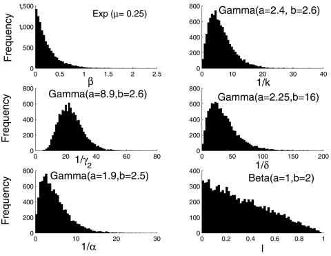
We carried out an uncertainty analysis on the basic reproductive number (R₀) to assess the variability in R₀ that results from the uncertainty in the model parameters. We used a Monte Carlo procedure (simple random sampling) to quantify the uncertainty of R₀ to model parameters when these parameters are distributed. Similar methods have been used before (12–14). Parameters (k, γ₂, δ, α) were assigned a different probability density function (PDF) (Figure 1), which is taken from reference 3. The relative measure of infectiousness of persons after isolation procedures are put in place (l) was assumed to be uniformly distributed in the interval (0 < l < 1). The observed heterogeneity in transmission rates during the SARS epidemic is modeled here by assuming that β is distributed exponentially with mean 0.25 person^–1 day^–1 (our estimate of the transmission rate in Hong Kong). Parameters q, p, and ρ are fixed to their baseline values (Table 1). We sampled the set of six parameters (β, k, γ₂, δ, α, l) 10⁵ times, holding q, p, and ρ fixed. We then computed R₀ from each set. A probability density function for R₀ is obtained and can be statistically characterized. Here, we characterize R₀ by its median and interquartile range.

Figure 1.

Histograms of the six distributed parameters appearing in equation 1 with sample size 10⁵. The transmission rate was assumed to be exponentially distributed with mean 0.25, our estimated transmission rate in Hong Kong. Here l is assumed to have a beta distribution (l ~ β [1,2]). Alternative distributions for l were also used as described in the text. All other distributions were taken from reference 3.

Sensitivity Analysis for R₀

We performed a sensitivity analysis on R₀ to quantify the effect of changes in the model parameters on R₀. Hence, we rank model parameters according to the size of their effect on R₀. Partial rank correlation coefficients (12–15) were computed between each of the parameters (with the exception of p, q, and ρ, which were held fixed) and R₀ as samples were drawn from the distributions, thus quantifying the strength of the parameter's linear association with R₀. The larger the partial rank correlation coefficient, the larger the influence of the input parameter on the magnitude of R₀. Because the distribution of the parameter l (relative infectiousness after isolation) is not known, we also studied the sensitivity of R₀ to various distributions of l. Distributions of l used for the Monte Carlo calculation of the partial rank correlation coefficients are: a) l ~ β (a = 2, b = 2) where β is used to denote a beta distribution. Here, the likelihood of l is bell-shaped with mean 0.5 and variance 0.05; b) l ~ β (a = 1, b = 2), the likelihood of l decreases linearly in the [0,1] interval; and c) l ~ β (a = 2, b = 1), the likelihood of l increases linearly in the [0,1] interval.

Results

Uncertainty Analysis for R₀

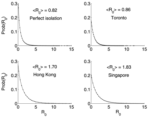
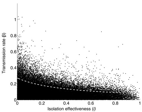
The resulting R₀ distribution lies in the interquartile range 0.43–2.41, with a median of 1.10. Moreover, the probability that R₀ > 1 is 0.53. The same Monte Carlo procedure, but with fixed values of l = 0.1 and α = 1/3 day^–1 for Toronto (i.e., after implementing control measures on March 26), give a median and interquartile range for the distribution of R₀ = 0.58 (0.24–1.18) (Table 2). Similarly, a lower rate of diagnosis a = 1/4.85 day^–1 and the relative infectiousness after isolation in Hong Kong (l = 0.43) and Singapore (l = 0.49) gives R₀ = 1.10 (0.44–2.29) and 1.17 (0.47–2.47), respectively (Figure 2). Perfect isolation (l = 0) gives R₀ = 0.49 (0.19–1.08). Especially noteworthy is that even in cases when eventual control of an outbreak is achieved (Toronto and a hypothetical case of perfect isolation), 25% of the weight of the distribution of R₀ lies at R₀ > 1. Furthermore, the median and interquartile range of R₀ are larger when p = 1, as has been assumed (8). In Figure 3 we show the (β, l) parameter space when R₀ < 1 obtained from our uncertainty analysis (14).

Table 2. The median and the interquartile range (IQR) of the distribution of the basic reproductive number (R₀) of SARS for Toronto, Hong Kong, and Singapore obtained from our uncertainty analysis.

Location	R0 mean	R0 median	R0 IQR
Toronto, Canada (l = 0.10)	0.86	0.58	0.24–1.18
Hong Kong (l = 0.43)	1.70	1.10	0.44–2.29
Singapore (l = 0.49)	1.83	1.17	0.47–2.47

Figure 2.

Empiric (dots) and stretched exponential estimated probability density function Prob(R₀) = a exp[–(R₀/b)^c] (solid line) (16) of R₀ for the cases of Toronto (a = 0.186, b = 0.803, c = 0.957, after control measures had been implemented), Hong Kong (a = 0.281, b = 1.312, c = 0.858), and Singapore (a = 0.213, b = 1.466, c = 0.883) obtained from our uncertainty analysis. The distribution for the case of perfect isolation (l = 0, a = 0.369, b = 0.473, c = 0.756) is shown as a reference.

Figure 3.

(β, l) parameter space when R₀ < 1 obtained from the uncertainty analysis (black dots). The deterministic (β, l) level curve when R₀ = 1 is shown in by the dotted white line. All other parameters in equation 1 were fixed to their baseline values (Table 1). l = 0 denotes perfect isolation; l = 1 denotes no isolation.

Sensitivity Analysis for R₀

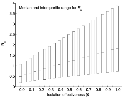
The transmission rate β and the relative infectivity during isolation (l) are the most influential parameters in determining R₀. The systematic decline in R₀ with increasing l in the range [0,1] is illustrated in Figure 4. Furthermore, our results do not change if we assume the three distributions mentioned in the Methods section (sensitivity analysis) for the parameter l. Table 3 shows the partial rank correlation coefficients for the other three possible distributions of l. The transmission rate is ranked first independent of the distribution of l. The relative infectiousness after isolation is ranked second when l comes from distributions (a) and (b) and ranked third when it comes from distribution (c) (see Methods). Our sensitivity analysis is corroborated by computing local derivatives on R₀ (see Appendix). Because bounds exist on how much a given parameter can change in practice, achieving control (i.e., R₀ < 1) can require changing parameters other than those with the highest partial rank correlation coefficient. For example, reference 10 showed that control of the outbreak in Toronto relied on both a reduction in l and 1/α, even though α is ranked fairly low by the partial rank correlation coefficient.

Figure 4.

Boxplot of the sensitivity of R₀ estimates to varying values of l, the relative infectiousness after isolation has begun. l = 0 denotes perfect isolation while l = 1 denotes no isolation. The boxplot shows the median and the interquartile range of R₀ obtained from Monte Carlo sampling of size 10⁵.

Table 3. Partial rank correlation coefficients (PRCCs) between each of the input parameters and R₀ from Monte Carlo sampling of size 10⁵ for different distributions of the relative infectiousness after isolation (l) as described in the text.

Probability distribution	Input parameters in order of decreasing PRCC (shown in parenthesis)
β (a = 2, b = 2)	β (0.92), l (0.57), δ (0.53), γ2 (0.35), α (0.32), k (0.13)
β (a = 1, b = 2)	β (0.90), l (0.60), δ (0.44), α (0.39), γ2 (0.26), k (0.12)
β (a = 2, b = 1)	β (0.92), δ (0.60), l (0.51), γ2 (0.40), α (0.22), k (0.11)

Conclusion

We have estimated R₀ for the cases of Toronto, Hong Kong, and Singapore (Table 2) through an uncertainty analysis shown in equation 1. Our estimates for R₀ agree with the empirical R₀ observed from the data of the first week of the SARS outbreak in Singapore (8). A stretched exponential distribution fits the resulting distributions of R₀ for the different locations (Figure 2). Even though the median of R₀ is <1 when perfect patient isolation is assumed (l = 0), we find that 25% of our R₀ distribution lies at R₀ > 1. That is, implementing a single method for control may not be sufficient to contain a SARS outbreak. Control may require modifying more than one parameter amenable to intervention. In our model, these parameters include the diagnostic rate (α), the relative infectiousness after isolation has begun (l), and the per capita transmission rate (β). The fact that α and l are not independent, but are tightly coupled, favors control.

Our expression for R₀ incorporates the effects of diagnosis-isolation strategies. Moreover, our approach includes differential susceptibility (p) and effective population size (ρ). Most models take p = 1, even though data from Hong Kong show that a low-risk subpopulation lies in the age range <19, approximately 23% of Hong Kong's population (3). The assumption p = 1 thus overestimates R₀.

Our sensitivity analysis shows that the transmission rate (β) and the relative infectiousness after isolation in hospitals (l) have the largest effect on R₀. With the exception of a few measures, such as closing schools, no clear policies would modify β directly. This means that a substantial effort must be (and has been) made by the medical community to modify other parameters, such as the diagnostic rate. Hence, the strong sensitivity of R₀ to the transmission rate β indicates that efforts in finding intervention strategies that manage to systematically lower the contact rate of persons of all age groups promise an effective means for lowering R₀. Such strategies may include using face masks (the probability of transmission per contact may be reduced), washing hands, and avoiding large crowds (large public events).

Associated with the role of screening, diagnosis, and the effective isolation of patients is the issue of cost. We cannot ignore or minimize the value of stringent quarantine measures and the probability of compliance combined with the economic effect of lost wages (thousands were quarantined in Taiwan, Hong Kong, and Singapore [17]), the costs associated with screening at airports and hospitals, the cost associated with closing hospitals; and the costs associated with isolating SARS patients and exposed persons (see Appendix for a brief discussion).

Appendix

Local Sensitivity Analysis of the Basic Reproductive Number

The sensitivity analysis approach through an exhaustive sampling of the parameter space provides a global measure of the sensitivity of model parameters. Another approach is to compute the sensitivity indices of the model parameters through local derivatives (18). This approach only provides a local measure as the sensitivity indices can change when the parameter values change. Here, we use local sensitivity analysis to corroborate our global sensitivity analysis results and discuss how this approach can be applied in the analysis of cost as part of a policy of outbreak control.

Let λ represent any of the 10 nonnegative parameters, β, ρ, p, q, k, γ₁, γ ₂, δ, α, and l, that define the basic reproductive number of our model (19)

(1)

If a "small" perturbation δλ is made to the parameter λ, a corresponding change will occur in R₀ as δR₀, where

The normalized sensitivity index Ψ_λ is the ratio of the corresponding normalized changes and is defined as

(2)

An approximation of the perturbed value of R₀, in terms of the sensitivity index is

where the 10 normalized sensitivity indexes are

with η = p(1–ρ)+ρ and γ₂ = a γ₁/( α –γ₁). For the values of the parameters used in this model, the sensitivity indices Ψ_β, Ψ_ρ, Ψ_p, Ψ_q, and Ψ_l are positive, Ψ_k = –Ψ_q, and the remaining indexes are negative. Furthermore, since all of the indexes (except Ψ_β) are functions of the parameters, the sensitivity indexes will change as the parameter values change.

For our specific case where β = 0.25, q = 0.1, p = 1/3, k = 0.15707, α = 0.2061, γ₁ = 0.035285, γ₂ = 0.0426, δ = 0.0279, and ρ = 0.77 and Toronto (l = 0.1) or Hong Kong (l = 0.43), the normalized sensitivity indices are computed. The sensitivity indices and the associated percentage changes needed to affect a 1% decrease in R₀ are given in Tables A1 and A2. Since the effective rate of patient isolation and the average rate of diagnosis are two feasible intervention strategies, we examine how changes to the parameters l and α affect R₀.

Let us first consider the outbreak in Hong Kong. The value α = 0.2061 means that the mean time to diagnose an infected person's illness is approximately 4.85 days. The sensitivity index Ψ_α = –0.1933 means that a 5.2% increase in α, which in turn requires a decrease of 5.7 hours of mean time to diagnosis, would result in a decrease of approximately 1% in R₀. Similarly, the sensitivity index Ψ_l = 0.5183 suggests that a 1.9% decrease in the value of l, that is going from 0.43 to 0.42 isolation effectiveness,2 results in a 1% decrease in R₀. In other words, individually a 5.2% increase in a or a 1.9% decrease in l both result in approximately a 1% decrease in R₀. For the particular values of the parameters chosen for Hong Kong, the most effective way to reduce R₀ is to decrease the transmission rate β and the parameter l (improve the effective isolation rate). In the case of Toronto, Ψ_α = –0.4758 means that a 2.1% increase in α, results in a 1% decrease in R₀, whereas Ψ_l = 0.2001 means a 5% decrease in l also results in a 1% decrease in R₀.

As can be seen from these two examples, the importance or ranking of the sensitivity indices can change as the values of the parameters change. Specifically, the sensitivity indices Ψ_l and Ψ_α satisfy the relationship

(3)

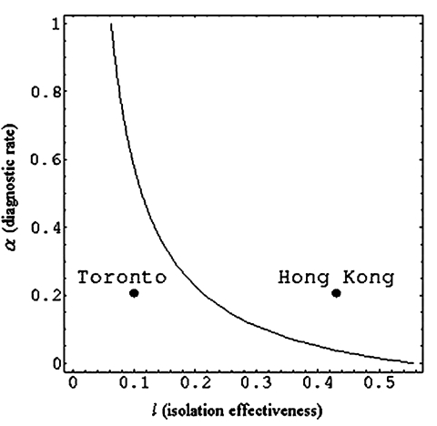
For the particular values of the parameters given above, the Figure A1 shows the level curve for the pair (l,α), where l(α+2γ₁+2δ) = δ+γ₂. The particular parameter values are either for Toronto (l,α) = (0.1, 0.2064) or for Hong Kong (l,α) = (0.43, 0.2064). Choosing the parameter values (l,α) below the level curve means that ||Ψ_l|| < ||Ψ_α||and the converse is true if (l,α) is chosen above the curve. Along the level curve, the magnitude of the sensitivities is equal. Notice that the level curve divides the parameter space into two regions, each of area A_above and A_below, respectively. Since A_above >> A_below, Ψ_l will be the dominant sensitivity index for randomly chosen (l,α).

One aspect of implementing an efficient intervention policy is the fact that limited resources are available. If one assumes, for example, that the strategies of isolation and diagnosis have associated 1% incremental costs in implementation of δC_I and δC_D, respectively, then a mixed strategy should be formulated that maximizes the effectiveness of a combined intervention. Specifically, if x denotes the magnitude of percentage decrease in l, and y denotes the % increase in a and assuming that there is a maximum amount of total additional resources available (δC_T), then the total additional cost of a new mixed isolation and diagnosis intervention policy must satisfy the inequality δC_Ix+δC_Dy < δC_T. Since the objective is to maximize the decrease in R₀, this means we want to maximize the objective function P = ||Ψ_l||x+||Ψ_α||y under the appropriate constraints. In a more general setting, additional nonlinear constraints could be involved, which case would require one to solve a nonlinear optimization problem. The situation in which the cost of diagnosis of infected persons may be much greater than the cost of isolation or vice versa is certainly of interest.

Biography

Mr. Chowell is a Ph.D. candidate in the department of Biological Statistics and Computational Biology at Cornell University. His research interests include epidemic modeling of emerging infectious diseases and social network analysis.

Table A1. Sensitivity indices for Toronto with l = 0.1.

Positive sensitivity indices		Negative sensitivity indices
Ψβ = 1	–1%	Ψα = –0.4758	2.10%
Ψr = 0.6063	–1.65%	Ψδ = –0.1707	5.86%
Ψl = 0.2001	–4.99%	Ψγ2 = –0.1208	8.28%
Ψγ = 0.1172	–8.53%	Ψk = –0.1172	8.53%
Ψp = 0.0906	–11.04%	Ψγ1 = –0.1156	8.65%

Table A2. Sensitivity indices for Hong Kong with l = 0.43.

Positive sensitivity indices		Negative sensitivity indices
Ψβ = 1	–1%	Ψγ2 = –0.3129	3.19%
Ψρ = 0.6063	–1.65%	Ψδ = –0.3016	3.32%
Ψl = 0.5183	–1.93%	Ψα = –0.1933	5.17%
Ψp = 0.0906	–11.04%	Ψγ1 = –0.1216	8.22%
Ψq = 0.0706	–14.16%	Ψk = –0.0706	14.16%

Figure A1.

Level curve of (l,α), where l(α+2γ₁+2δ) = δ+γ₂.

References

- 1.Kamps BS, Hoffmann C, eds. SARS Reference [monograph on the Internet]. 3rd ed. 2003. Oct [cited 2003 Jul 5]. Available from: http://www.sarsreference.com/sarsref/summary.htm
- 2.World Health Organization. Cumulative number of reported probable cases of severe acute respiratory syndrome (SARS) [monograph on the Internet]. [cited 2003 Jul 5]. Available from: http://www.who.int/csr/sarscountry/en/
- 3.Donnelly CA, Ghani AC, Leung GM, Hedley AJ, Fraser C, Riley S, et al. Epidemiological determinants of spread of causal agent of severe acute respiratory syndrome in Hong Kong. Lancet. 2003;361:1761–6. 10.1016/S0140-6736(03)13410-1 [DOI] [PMC free article] [PubMed] [Google Scholar]
- 4.Vogel G. Flood of sequence data yields clues but few answers. Science. 2003;300:1062. 10.1126/science.300.5622.1062a [DOI] [PubMed] [Google Scholar]
- 5.Booth CM, Matukas LM, Tomlinson GA, Rachlis AR, Rose DB, Dwosh HA, et al. Clinical features and short-term outcomes of 144 patients with SARS in the greater Toronto area. JAMA. 2003;289:2801–9. 10.1001/jama.289.21.JOC30885 [DOI] [PubMed] [Google Scholar]
- 6.Health chief says 94 percent of SARS cases result of hospital infections [news release on the Internet]. Taiwan Headlines. 2003. May 20 [cited 2003 Jul 5]. Available from: http://www.taiwanheadlines.gov.tw/20030520/20030520s1.html
- 7.World Health Organization. Update 28 – affected areas, status of SARS outbreaks in individual countries [monograph on the Internet]. 2003. Apr 12 [cited 2003 20 May]. Available from: http://www.who.int/csr/sarsarchive/2003_04_12/en/
- 8.Lipsitch M, Cohen T, Cooper B, Robins JM, Ma S, James L, et al. Transmission dynamics and control of severe acute respiratory syndrome. Science. 2003;300:1966–70. 10.1126/science.1086616 [DOI] [PMC free article] [PubMed] [Google Scholar]
- 9.Riley S, Fraser C, Donnelly CA, Ghani AC, Abu-Raddad LJ, Hedley AJ, et al. Transmission dynamics of the etiological agent of SARS in Hong Kong: impact of public health interventions. Science. 2003;300:1961–6. 10.1126/science.1086478 [DOI] [PubMed] [Google Scholar]
- 10.Chowell G, Fenimore PW, Castillo-Garsow MA, Castillo-Chavez C. SARS outbreaks in Ontario, Hong Kong and Singapore: the role of diagnosis and isolation as a control mechanism. J Theor Biol. 2003;224:1–8. 10.1016/S0022-5193(03)00228-5 [DOI] [PMC free article] [PubMed] [Google Scholar]
- 11.Brown D. A model of epidemic control. The Washington Post. 2003. May 3. p. A07.
- 12.Sanchez MA, Blower SM. Uncertainty and sensitivity analysis of the basic reproductive rate: tuberculosis as an example. Am J Epidemiol. 1997;145:1127–37. [DOI] [PubMed] [Google Scholar]
- 13.Blower SM, Dowlatabadi H. Sensitivity and uncertainty analysis of complex models of disease transmission: an HIV model, as an example. Int Stat Rev. 1994;2:229–43. 10.2307/1403510 [DOI] [Google Scholar]
- 14.Velasco-Hernandez JX, Gershengorn HB, Blower SM. Could widespread use of combination antiretroviral therapy eradicate HIV epidemics? Lancet Infect Dis. 2002;2:487–93. 10.1016/S1473-3099(02)00346-8 [DOI] [PubMed] [Google Scholar]
- 15.Kendall MG, Stuart A. The advanced theory of statistics. 4th ed. New York: Macmillan Publishing Co.; 1979. [Google Scholar]
- 16.Kohlrausch R. Ann Phys (Leipzig). 1847;12:393–8. [Google Scholar]
- 17.Mandavilli A. SARS epidemic unmasks age-old quarantine conundrum. Nat Med. 2003;9:487. 10.1038/nm0503-487 [DOI] [PMC free article] [PubMed] [Google Scholar]
- 18.Caswell H. Matrix population models. 2nd ed. Sunderland (MA): Sinauer Associates, Inc. Publishers; 2001. [Google Scholar]
- 19.Chowell G, Fenimore PW, Castillo-Garsow MA, Castillo-Chavez C. SARS outbreaks in Ontario, Hong Kong, and Singapore: the role of diagnosis and isolation as a control mechanism. J Theor Biol. 2003;224:1–8. 10.1016/S0022-5193(03)00228-5 [DOI] [PMC free article] [PubMed] [Google Scholar]