Denoising Sparse Images from GRAPPA using the Nullspace Method (DESIGN)

Abstract

To accelerate magnetic resonance imaging using uniformly undersampled (nonrandom) parallel imaging beyond what is achievable with GRAPPA alone, the Denoising of Sparse Images from GRAPPA using the Nullspace method (DESIGN) is developed. The trade-off between denoising and smoothing the GRAPPA solution is studied for different levels of acceleration. Several brain images reconstructed from uniformly undersampled k-space data using DESIGN are compared against reconstructions using existing methods in terms of difference images (a qualitative measure), PSNR, and noise amplification (g-factors) as measured using the pseudo-multiple replica method. Effects of smoothing, including contrast loss, are studied in synthetic phantom data. In the experiments presented, the contrast loss and spatial resolution are competitive with existing methods. Results for several brain images demonstrate significant improvements over GRAPPA at high acceleration factors in denoising performance with limited blurring or smoothing artifacts. In addition, the measured g-factors suggest that DESIGN mitigates noise amplification better than both GRAPPA and L₁ SPIR-iT (the latter limited here by uniform undersampling).

Introduction

The time-consuming nature of image encoding in magnetic resonance imaging (MRI) continues to inspire novel acquisition and image reconstruction techniques and technologies. In conventional Cartesian Fourier transform-based imaging, 3-D k-space is sampled along readout lines uniformly spaced in the phase-encode directions. To reduce the scan time, accelerated parallel imaging uses multiple receiver coils to produce high-quality images without aliasing from k-space acquisitions that are undersampled in the phase-encode directions.

To obtain superior image reconstructions from even less data than is possible with multiple receiver coils alone, we investigate combining sparsity-promoting regularization with the GRAPPA accelerated parallel imaging reconstruction method (1). GRAPPA directly estimates the missing k-space lines in all the coils from the undersampled data, using a set of specially calibrated reconstruction kernels. The proposed method uses a combination of a weighted fidelity to the GRAPPA reconstruction, a joint sparsity penalty function, and a data-preserving nullspace formulation. This method is designed to accommodate uniform Cartesian sampling patterns and can be implemented with similar complexity to existing sparsity regularization methods; in addition, this method can be easily adapted to random Cartesian subsampling by modifying only the GRAPPA reconstruction step, although this extension is not studied here.

Accelerated parallel imaging

Given multiple receiver coils, post-processing techniques like SENSE (2), SMASH (3), GRAPPA, and SPIR-iT (4), synthesize un-aliased images from multi-coil undersampled data, in either k-space or the image domain. GRAPPA and SPIR-iT acquire several additional k-space lines, called ACS lines, to form kernels for use in reconstruction. One important limitation of GRAPPA is the assumption of uniform undersampling. However, GRAPPA can be extended to non-uniform Cartesian subsampling at greater computational cost by using many kernels, one for each source/target pattern encountered. In contrast, SPIR-iT easily accommodates non-uniform sampling patterns, since SPIR-iT uses the kernel to enforce consistency between any point in k-space and its neighborhood of k-space points, both acquired and unknown. All these methods successfully reconstruct diagnostically useful images from undersampled data; however, at higher acceleration factors, GRAPPA tends to fail due to noise amplification or incompletely resolved aliasing. Due to its indirect formulation, SPIR-iT is more computationally intensive than GRAPPA for uniform undersampling.

Sparsity-enforcing regularization of parallel imaging

Since a wide variety of MR images are approximately sparse (5), the compressed sensing (CS) (6–8) framework is a reasonable alternative for recovering high-quality images from undersampled k-space. However, remaining faithful to uniform undersampling destroys the incoherent sampling (with respect to the sparse transform domain) useful for CS. Applying CS or methods combining parallel imaging and CS like L₁ SPIR-iT (9,10) to uniformly undersampled data results in images with noticeable coherent aliasing artifacts. Since the noise amplified by parallel imaging methods like GRAPPA remains unstructured in the sparse transform domain regardless of the k-space sampling pattern, sparsity-enforcing regularization nevertheless can improve image quality in the uniformly undersampled case via denoising. This combination of GRAPPA and sparsity-based denoising remains not fully explored. This work, of which a preliminary account is presented in (11), succeeds CS-GRAPPA (12), L₁ SPIR-iT, CS-SENSE (13), and other joint optimization approaches. It combines GRAPPA with sparsity regularization to enable quality reconstructions from scans with greater acceleration where noise amplification dominates the reconstruction error.

CS-GRAPPA, CS-SENSE, and L₁ SPIR-iT all combine parallel imaging methods (GRAPPA, SENSE, and SPIR-iT) with compressed sensing, but each differs from the proposed method (beyond undersampling strategies). CS-GRAPPA combines CS and GRAPPA, alternatingly applying GRAPPA and CS reconstructions to fill the missing k-space lines; the iterative structure of this method may limit the synergy between sparsity and multiple coils. CS-SENSE sequentially applies CS to each aliased coil image and combines the CS results using SENSE; like SENSE, CS-SENSE is highly sensitive to the quality of the estimates of the coil sensitivity profiles. L₁ SPIR-iT is the most similar to the proposed method, as it jointly optimizes both for sparsity and for fidelity to a parallel imaging solution. However, L₁ SPIR-iT iteratively applies the SPIR-iT kernel, updating the k-space data for consistency instead of filling in the missing k-space data directly. The presented algorithm uses a direct GRAPPA reconstruction and applies sparsity as a post-processing method for denoising.

The proposed method—Denoising Sparse Images from GRAPPA using the Nullspace method (DESIGN)—jointly optimizes a GRAPPA fidelity penalty and simultaneous sparsity of the coil images while preserving the data by optimizing in the nullspace of the data observation matrix. The effects of adjusting the tuning parameter balancing sparsity and GRAPPA fidelity are evaluated. The resulting algorithm is compared against GRAPPA alone and other denoising methods, to measure the additional improvement possible from combining these accelerated image reconstruction techniques, as well as against L₁ SPIR-iT, the prevailing method combining parallel imaging and CS (albeit here with uniform undersampling).

Theory

GRAPPA

In this work, we assume that the 3-D acquisition is accelerated in only the phase-encode directions, so the volume can be divided into 2-D slices in the readout direction and each slice reconstructed separately. Thus, GRAPPA and SPIR-iT are presented for 2-D accelerated data with 2-D calibration data; this formulation follows the “hybrid space CCDD method” with “independent calibration” discussed in (14); other formulations are certainly possible.

For a given slice, denote the 2-D k-space value at frequency (k_y,k_z) encoded by the pth coil as y_p(k_y,k_z), the frequency spacing corresponding to full field-of-view (FOV) sampling (Δk_y, Δk_z), the number of coils P, and the size of the correlation kernel (B_y,B_z). In GRAPPA, the missing data is recovered using

$$y_p(k_y+r_y\mathrm{\Delta }{k}_y,k_z+r_z\mathrm{\Delta }{k}_z)={\displaystyle \sum _{q=1}^P}{\displaystyle \sum _{b_y=1}^{B_y}}{\displaystyle \sum _{b_z=1}^{B_z}}{g}_q^{(p,r_y,r_z)}(b_y,b_z)y_q(k_y+(b_y-\lceil \frac{B_y}{2}\rceil )R_y\mathrm{\Delta }{k}_y,k_z+(b_z-\lceil \frac{B_z}{2}\rceil )R_z\mathrm{\Delta }{k}_z),$$ [1]

where the kernel coefficients $g_q^{\left(p,r_y,r_z\right)}\left(b_y,b_z\right)$ are computed from a least-squares fit using the ACS lines in that slice. Let M and N represent the number of acquired and full k-space data points in a coil slice, respectively; the M × P matrix D is the acquired data for all the coils, and the N × P matrix Y is the full k-space for all the coils. Collecting the GRAPPA reconstruction equations for the full k-space yields the full k-space reconstruction Y_GRAPPA = G(D), where G is a linear system that can be implemented efficiently using convolutions.

SPIR-iT

SPIR-iT uses a different kernel to form consistency equations for each point in the full k-space with its neighbors and organizes the resulting consistency equations into the linear system Y = G_S(Y); the complete derivation of the consistency kernel coefficients can be found in (4). SPIR-iT minimizes the ℓ₂ consistency error using the constrained optimization problem

$${\mathbf{Y}}_{\text{SPIR-iT}}\in \underset{\mathbf{Y}}{\text{minimize}}{\Vert \mathbf{Y}-{\mathbf{G}}_S(\mathbf{Y})\Vert }_F^2\mathrm{s}.\mathrm{t}.{\Vert \mathbf{D}-\mathbf{K}\mathbf{Y}\Vert }_F^2\le \epsilon ,$$ [2]

where K is the M × N subsampling matrix selecting the observed k-space data points, ‖·‖_F is the Frobenius norm, and ε constrains the allowed deviation from the data. When preserving the acquired data exactly (setting ε = 0 above), the SPIR-iT optimization problem is conveniently expressed in the nullspace of the subsampling matrix K (15). Let K^c represent the (N−M) × N subsampling matrix selecting the missing k-space. The range of [K^T,(K^c)^T] is R^N, and each row of K^c is in the nullspace of K. Thus, if the missing k-space data X = K^cY, then Y = K^TD + (K^c)^TX is a nullspace decomposition of Y. When the data is preserved with equality, the SPIR-iT optimization problem becomes

$${\mathbf{X}}_{\text{SPIR-iT}}\in \underset{\mathbf{X}}{\text{minimize}}{\Vert {\mathbf{K}}^{\mathrm{T}}\mathbf{D}+{\left({\mathbf{K}}^{\mathrm{c}}\right)}^{\mathrm{T}}\mathbf{X}-{\mathbf{G}}_S({\mathbf{K}}^{\mathrm{T}}\mathbf{D}+{\left({\mathbf{K}}^{\mathrm{c}}\right)}^{\mathrm{T}}\mathbf{X})\Vert }_F^2;{\mathbf{Y}}_{\text{SPIR-iT}}={\mathbf{K}}^{\mathrm{T}}\mathbf{D}+{({\mathbf{K}}^{\mathrm{c}})}^{\mathrm{T}}{\mathbf{X}}_{\text{SPIR-iT}}.$$ [3]

Augmenting the SPIR-iT optimization problem with the hybrid ℓ _2,1 norm of the sparsifying transform of the coil images and utilizing random undersampling of k-space yields the L₁ SPIR-iT method. Denote the regularization parameter λ, the sparsifying transform Ψ, and the inverse discrete Fourier transform F⁻¹; then the above optimization problem becomes

$${\mathbf{X}}_{{\mathrm{L}}_1\text{SPIR-iT}}\in \underset{\mathbf{X}}{\text{minimize}}{\Vert {\mathbf{K}}^{\mathrm{T}}\mathbf{D}+{\left({\mathbf{K}}^{\mathrm{c}}\right)}^{\mathrm{T}}\mathbf{X}-{\mathbf{G}}_S\left({\mathbf{K}}^{\mathrm{T}}\mathbf{D}+{\left({\mathbf{K}}^{\mathrm{c}}\right)}^{\mathrm{T}}\mathbf{X}\right)\Vert }_F^2+\lambda {\displaystyle \sum _{n=1}^N}{\Vert {\left[\mathbf{\Psi }{\mathbf{F}}^{-1}\left({\mathbf{K}}^{\mathrm{T}}\mathbf{D}+{\left({\mathbf{K}}^{\mathrm{c}}\right)}^{\mathrm{T}}\mathbf{X}\right)\right]}_{n,:}\Vert }_2.$$ [4]

DESIGN: combining GRAPPA and sparsity

To regularize GRAPPA with sparsity, the objective function consists of a least-squares term to favor fidelity to the GRAPPA k-space result and a function to promote simultaneous sparsity across the coil images in the sparse transform domain. Using the notation G(D) to denote the GRAPPA-reconstructed full k-space, λ for the tuning parameter trading off fidelity to the GRAPPA solution for sparsity, ‖·‖_s for the simultaneous sparsity penalty function, we have

$${\mathbf{Y}}_{\text{DESIGN}}\in \underset{\mathbf{Y}}{\text{minimize}}{\Vert \mathbf{Y}-\mathbf{G}(\mathbf{D})\Vert }_F^2+\lambda {\Vert \mathbf{\Psi }{\mathbf{F}}^{-1}\mathbf{Y}\Vert }_s\mathrm{s}.\mathrm{t}.\mathbf{D}=\mathbf{\text{KY}}.$$ [5]

Denote the sparse transform representation of a single vector w. To construct the simultaneous sparsity penalty function on the sparse transform matrix W, we first consider a single vector w and a separable approximation to the ℓ₀ “norm” ${\displaystyle {\sum }_{n=1}^N}s\left(w_n\right)$ For example, s(w_n) = |w_n| for the ℓ ₁ norm in (6,8), s(w_n) = |w_n|^p for the ℓ_p (p < 1) penalty in (16), or s(w_n) = log(1+|w_n|²) for the Cauchy penalty function (17). In this paper, the ℓ₁ norm is chosen due to its convexity and suitability for approximately sparse signals. Now, let W represent the sparse transform coefficients for a collection of vectors Y; W = ΨF⁻¹Y. To extend this sparsity penalty function to simultaneous sparsity across coil images, we consider s(w_n) applied to the ℓ₂ norm of the vector of sparse transform coefficients [W_n,1, …, W_n,P]:

$${\Vert \mathbf{W}\Vert }_s={\displaystyle {\sum }_{n=1}^N}S({\Vert [{\mathbf{W}}_{n,1}\cdots {\mathbf{W}}_{n,P}]\Vert }_2).$$ [6]

By enforcing simultaneous sparsity across the magnitudes of the sparse representations of all the coil images, we target the sparsity inherent in the combined image.

The GRAPPA reconstruction operations in k-space non-uniformly amplify the additive noise in the image domain. Coupled with correlation across channels, the GRAPPA reconstruction noise power varies in each voxel and across coils, so we replace the GRAPPA fidelity term with a weighted ℓ ₂ norm. Here, we weight the deviation from the GRAPPA result for each voxel in each coil by its contribution to the final combined image, with the notion that voxels with B₁⁻ attenuation (due to the receive coils’ sensitivities) or more noise amplification (due to GRAPPA) should be allowed to deviate more and contribute less to the final image. The multi-channel reconstructed images are combined as a post-processing step using per-voxel linear coil-combination weights C that are computed from an estimate of the coil sensitivity profiles. Due to the known smoothness of coil sensitivity profiles, this estimate is computed from low-resolution data. If the ACS lines are situated at the center of k-space (as is the case for the datasets evaluated in this paper), this calibration data is suitable for estimating the coil sensitivity profiles due to the known smoothness of those profiles. Otherwise, a sum-of-squares combination of the reconstructed coil images can be performed and the GRAPPA fidelity term is reweighted by just the coil noise covariance. Based on the formulation of the multi-channel SNR equation in (18) and SENSE, the coil combination weights are computed to be "signal normalized," i.e. the gain is unity. In particular, we employ the weights that combine the data across channels such that the resulting SNR is optimized (if the sensitivities are exact):

$$[C_1(x,y,z)\cdots C_P(x,y,z)]={({[\begin{array}{c}\hfill S_1(x,y,z)\hfill \\ \hfill ⋮\hfill \\ \hfill S_P(x,y,z)\hfill \end{array}]}^{\mathrm{H}}{\mathbf{\Lambda }}^{-1}\left[\begin{array}{c}\hfill S_1(x,y,z)\hfill \\ \hfill ⋮\hfill \\ \hfill S_P(x,y,z)\hfill \end{array}]\right)}^{-1}{[\begin{array}{c}\hfill S_1(x,y,z)\hfill \\ \hfill ⋮\hfill \\ \hfill S_P(x,y,z)\hfill \end{array}]}^{\mathrm{H}}{\mathbf{\Lambda }}^{-1},$$ [7]

where [·]^H is the conjugate transpose, S_p(x,y,z) are the coil sensitivity estimates, and Λ is the measured coil noise covariance matrix. Each voxel of the combined image is formed by multiplying the vector [C₁(x,y,z), …, C_P(x,y,z)] by the stacked vector of the corresponding pixel in all of the coil images. This combination corresponds to performing SENSE on un-accelerated data with low-resolution coil sensitivity estimates. Using these coil combination weights, DESIGN becomes

$${\mathbf{Y}}_{\text{DESIGN}}\in \underset{\mathbf{Y}}{\text{minimize}}{\Vert \mathbf{C}·{\mathbf{F}}^{-1}(\mathbf{Y}-\mathbf{G}(\mathbf{D}))\Vert }_F^2+\lambda {\Vert \mathbf{\Psi }{\mathbf{F}}^{-1}\mathbf{Y}\Vert }_s\mathrm{s}.\mathrm{t}.\mathbf{D}=\mathbf{\text{KY}}.$$ [8]

While not investigated here, one could also substitute analytical GRAPPA per-coil g-factors (based on the kernel) for the coil combination weights. However, the coil combination weights may already be available, as we use them to combine the full reconstructed k-space into a single combined image.

In order to solve this optimization problem, we first convert it to an unconstrained form using the aforementioned nullspace method:

$${\mathbf{X}}_{\text{DESIGN}}\in \underset{\mathbf{X}}{\text{minimize}}{\Vert \mathbf{C}·{\mathbf{F}}^{-1}({\mathbf{K}}^{\mathrm{T}}\mathbf{D}+{\left({\mathbf{K}}^{\mathrm{c}}\right)}^{\mathrm{T}}\mathbf{X}-\mathbf{G}(\mathbf{D}))\Vert }_F^2+\lambda {\Vert \mathbf{\Psi }{\mathbf{F}}^{-1}\left({\mathbf{K}}^{\mathrm{T}}\mathbf{D}+{\left({\mathbf{K}}^{\mathrm{c}}\right)}^{\mathrm{T}}\mathbf{X}\right)\Vert }_s.$$ [9]

The iteratively reweighted least squares (IRLS) method used in (19,20) is applied in conjunction with least-squares solver LSMR (21), available online at http://www.stanford.edu/group/SOL/software/lsmr.html. The IRLS method transforms the above problem into a succession of least-squares ones:

$${\mathbf{X}}^{t+1}\in \underset{\mathbf{X}}{\text{minimize}}{\Vert \mathbf{C}·{\mathbf{F}}^{-1}({\mathbf{K}}^{\mathrm{T}}\mathbf{D}+{\left({\mathbf{K}}^{\mathrm{c}}\right)}^{\mathrm{T}}\mathbf{X}-\mathbf{G}(\mathbf{D}))\Vert }_F^2+\lambda {\Vert {\mathbf{\Delta }}^{\frac{1}{2}}\left({\mathbf{X}}^t)\mathbf{\Psi }{\mathbf{F}}^{-1}\right({\mathbf{K}}^{\mathrm{T}}\mathbf{D}+{({\mathbf{K}}^{\mathrm{c}})}^{\mathrm{T}}\mathbf{X})\Vert }_F^2,$$ [10]

where the diagonal matrix [Δ(X)]_n,n = ∂s(w_n)/∂w_n /w_n for w_n = ‖W_n,:‖₂, and W = ΨF⁻¹(K^TD+(K^c)^TX); using this choice of reweighting matrix with IRLS is equivalent to using half-quadratic minimization (22–24). The gradient (or when s(·) is not differentiable, the sub-gradient) of the objective function is

$$2{\mathbf{K}}^{\mathrm{c}}{\mathbf{F}}^{-\mathrm{H}}({\mathbf{C}}^{*}·\mathbf{C}·{\mathbf{F}}^{-1}\left({\mathbf{K}}^{\mathrm{T}}\mathbf{D}+{({\mathbf{K}}^{\mathrm{c}})}^{\mathrm{T}}\mathbf{X}-\mathbf{G}(\mathbf{D}))\right)+2\lambda {\mathbf{K}}^{\mathrm{c}}{\mathbf{F}}^{-\mathrm{H}}{\mathbf{\Psi }}^{-\mathrm{H}}(\mathbf{\Delta }\left({\mathbf{X}}^t)\mathbf{\Psi }{\mathbf{F}}^{-1}\right({\mathbf{K}}^{\mathrm{T}}\mathbf{D}+{({\mathbf{K}}^{\mathrm{c}})}^{\mathrm{T}}\mathbf{X})),$$ [11]

where [·]^* is the element-wise complex conjugate. Setting the gradient equal to zero yields the linear system A^HAx = A^Hb, where x = vec(X), diag(·) constructs a diagonal matrix from a vector, ⊗ is the Kronecker product, and

$$\mathbf{A}=[\begin{array}{c}\hfill \text{diag}(\text{vec}(\mathbf{C}))\hfill \\ \hfill \sqrt{\lambda }({\mathbf{I}}_{P\times P}\otimes {\mathbf{\Delta }}^{\frac{1}{2}}\left({\mathbf{X}}^t)\mathbf{\Psi }\right)\hfill \end{array}]{\mathbf{I}}_{P\times P}\otimes {\mathbf{F}}^{-1}{({\mathbf{K}}^{\mathrm{c}})}^{\mathrm{T}},\text{ and }\mathbf{b}=[\begin{array}{c}\hfill \text{vec}(\mathbf{C}·{\mathbf{F}}^{-1}\left(\mathbf{G}(\mathbf{D})-{\mathbf{K}}^{\mathrm{T}}\mathbf{D})\right)\hfill \\ \hfill -\sqrt{\lambda }\text{ vec}({\mathbf{\Delta }}^{\frac{1}{2}}\left({\mathbf{X}}^t)\mathbf{\Psi }{\mathbf{F}}^{-1}{\mathbf{K}}^{\mathrm{T}}\mathbf{D}\right)\hfill \end{array}].$$ [12]

The IRLS method consists of fixing the diagonal weight matrix, solving the resulting linear system using LSMR, re-computing the weight matrix for the new vector x, and repeating until convergence. Solving the normal equations A^HAx = A^Hb using LSMR only requires that the matrix-vector multiplications Ax and A^Hy be efficient to compute for arbitrary vectors x and y.

Design choices

Before applying DESIGN denoising, a couple important design choices must be considered. Based on the class of images, an appropriate sparsifying transform must be chosen. Empirical evidence presented in (5) suggests that a wavelet or finite-differences transform yields approximately sparse representations for many types of MRI data, including brain images. Multi-scale multi-orientation transforms like the curvelet (25), contourlet (26), or shearlet (27) may improve sparsity; however, the extension of DESIGN to overcomplete transforms is not discussed here. In addition, the optimal choice of tuning parameter should be determined, based on the expected noise amplification and sparsity of the desired image.

Methods

In practical applications of DESIGN, data is acquired using a uniform subsampling of Cartesian k-space. A small set of ACS lines are acquired and are used to compute the 3×3 GRAPPA kernel (the 2-D kernel is the size of three neighboring k-space blocks in each direction), to generate coil combination weights, and to include as known data in the reconstruction. Before computing the sensitivity profiles, the ACS lines are apodized using a Blackman window that reduces the effects of low-resolution blurring on the profile estimates. The noise covariance matrix Λ is measured via a noise-only acquisition (no RF excitation) collected before the main acquisition; the noise covariance matrix is computed using the sample covariance across the coils of all the k-space samples.

Once the data is acquired, slices orthogonal to the readout direction are reconstructed individually using GRAPPA and the DESIGN algorithm, using design parameters appropriate for the acquisition. The optimization problem is solved using IRLS, combined with LSMR for inverting linear systems. Pseudocode for the complete algorithm is shown in Table 1. Each inner iteration of LSMR requires 2P FFT's, P fast sparsifying transforms, and its transpose, as well as multiplication by diagonal weight matrices and subsampling matrices. Although b (on the right side of the normal equation) only needs to be re-computed when the weight matrix changes, computing b has similar complexity. Thus, the overall algorithm's complexity is comparable to existing sparsity-based denoising methods. Since the time-consuming operations (FFT, wavelet, etc.) can be parallelized on a GPU, an efficient implementation suitable for practical use is possible.

Table 1.

Pseudocode for proposed method, DESIGN.

Estimate coil sensitivities from low-resolution data, and compute C. Compute GRAPPA kernel and run GRAPPA reconstruction on data D to yield result G(D). Initialization: X ← initial guess (possibly from GRAPPA result or previous run of method). $w_n\leftarrow {\Vert {\mathbf{\Psi }}_{n,:}{\mathbf{F}}^{-1}\left({\mathbf{K}}^{\mathrm{T}}\mathbf{D}+{({\mathbf{K}}^{\mathrm{c}})}^{\mathrm{T}}\mathbf{X}\right)\Vert }_2,{[\mathbf{\Delta }]}_{n,n}\leftarrow \frac{1}{w_n}\frac{\partial s(w_n)}{\partial w_n}$ $\mathbf{A}=\left[\begin{array}{c}\hfill \text{diag}(\text{vec}(\mathbf{C}))\hfill \\ \hfill \sqrt{\lambda }\left({\mathbf{I}}_{P\times P}\otimes {\mathbf{\Delta }}^{\frac{1}{2}}\mathbf{\Psi }\right)\hfill \end{array}\right]{\mathbf{I}}_{P\times P}\otimes {\mathbf{F}}^{-1}{({\mathbf{K}}^c)}^{\mathrm{T}},\mathbf{b}=\left[\begin{array}{c}\hfill \text{vec}(\mathbf{C}·{\mathbf{F}}^{-1}(\mathbf{G}(\mathbf{D})-{\mathbf{K}}^{\mathrm{T}}\mathbf{D}))\hfill \\ \hfill -\sqrt{\lambda }\text{vec}\left({\mathbf{\Delta }}^{\frac{1}{2}}\mathbf{\Psi }{\mathbf{F}}^{-1}{\mathbf{K}}^{\mathrm{T}}\mathbf{D}\right)\hfill \end{array}\right],\mathbf{X}\leftarrow \text{LSMR}(\mathbf{A},\mathbf{b})$ Repeat steps 4–5 until convergence. Full k-space result: Y ← KTD + (Kc)T X. Combined image: $\mathbf{I}\leftarrow {\displaystyle {\sum }_{p=1}^P}{[\mathbf{C}·{\mathbf{F}}^{-1}\mathbf{Y}]}_{:,p}.$

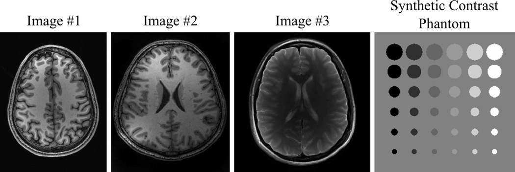
For the experiments that follow, several full-FOV 3-D datasets are acquired using un-accelerated sequences on Siemens Tim Trio 3 T systems (Siemens Healthcare, Erlangen, Germany) with the vendor 32-channel head-coil array. Two T₁-weighted MPRAGE’s (both 256×256×176 sagittal, 1.0 mm isotropic) and a T₂-weighted TSE (264×256×23 axial, 0.75×0.78×5 mm) all were collected, with acquisition times of 8, 8, and 4 minutes, respectively. From each of these datasets, a 2-D axial slice is extracted (and for the first two datasets, cropped); sum-of-squares combinations of these cropped images are used as the ground-truth. Slices from these three datasets and a synthetic phantom for studying contrast loss, are shown in Figure 1. Multiple channels were generated for the synthetic data using the Biot-Savart B₁ simulator written by Prof. Fa-Hsuan Lin available online at http://www.nmr.mgh.harvard.edu/~fhlin/tool_b1.htm. To generate the reduced-FOV data, each slice is undersampled in both directions in k-space. A 36×36 block (not undersampled) at the center of k-space is retained as the ACS lines used in the reconstructions; the total (effective) acceleration R accounts for this additional block of data. Based on empirical results in the literature (5), a four-level ‘9-7’ wavelet transform (DWT) is selected as an appropriate sparsifying transform for these images. This data is processed using the different reconstruction and denoising algorithms implemented in MATLAB. Each reconstructed image is evaluated qualitatively by generating a difference image and quantitatively by computing the peak-signal-to-noise ratio (PSNR):

$$\text{PSNR}=20{\text{ log}}_{10}\frac{\text{max}(|\text{ref}.\text{ image}|)}{\sqrt{\frac{1}{N}{\displaystyle \sum }{||\text{recon}.\text{ image}|-|\text{ref}.\text{ image}||}^2}}\text{ dB}.$$ [13]

Figure 1.

Sum-of-squares magnitude images of 2-D axial slices from three fully sampled brain (T1-weighted, normalized; T1-weighted, normalized; and T2-weighted, un-normalized) datasets, and a synthetic noise-free contrast phantom. These images are used as reference images (ground truth) for the difference images and magnitude-PSNR calculations shown throughout this paper.

Both the difference images and the PSNR are computed from magnitude images. As PSNR does not account for the importance of specific image features or the preservation of certain anomalies like tumors, the included difference images are used to understand the algorithms’ relative performances.

Optimizing the tuning parameter

In order to denoise a dataset using DESIGN, one must select a value of λ that achieves the desired trade-off between GRAPPA fidelity and sparsity. The sparsity penalty can be viewed as regularization, as it denoises the GRAPPA reconstruction. In this experiment, the effect of varying λ is studied for a single dataset and different acceleration factors. As tuning parameter selection is common to many regularization problems, inspiration for choosing an appropriate value can be drawn from the literature, including cross-validation for the lasso (28) or reference image-based L-curve selection for parallel imaging (29). Since the noise amplification of GRAPPA, and accelerated parallel imaging in general, is tied to the undersampling factor, the noise in the data, and the sparsity of the image, the choice of tuning parameter, λ, varies from image to image and acquisition to acquisition. For each acceleration, DESIGN is run for a coarse range of λ from 10^a, for a = −5, −4, …, 5, and 6, and repeated for densely-spaced λ around the optimal coarse value to determine the best value. The optimal choice of λ is determined for each dataset independently in the performance comparisons to follow.

Performance comparisons

To evaluate the performance of DESIGN, the implementation using the DWT (4-level 9-7 wavelet) sparsifying transform with the ℓ ₁ norm is compared against GRAPPA, GRAPPA with multichannel adaptive Wiener filter-based denoising, and L₁ SPIR-iT (admittedly limited by uniform undersampling). The multichannel Wiener filter-based denoising is approximated by (i) estimating a global noise variance on the combined image using median absolute deviation (30), (ii) estimating the local signal mean and variance for each pixel of the combined image, (iii) generating signal and noise covariances across coils using low-resolution coil sensitivities estimated from the ACS lines, and (iv) denoising each pixel of the uncombined data using the resulting multichannel Wiener filter. The implementation of L₁ SPIR-iT used in this paper is developed in (10), which is available online at http://www.cs.berkeley.edu/~mjmurphy/l1spirit.html. Various sizes of the SPIR-iT kernel are simulated, but little difference is observed between them; a 7×7 kernel (SPIR-iT kernel size refers to k-space points, not blocks) is used here. These performance experiments are repeated for various accelerations for a representative slice from each dataset. For L₁ SPIR-iT, the regularization parameter λ is chosen for each acceleration factor via the same parameter sweep approach as for DESIGN for each dataset.

Eliminating noise covariance estimation

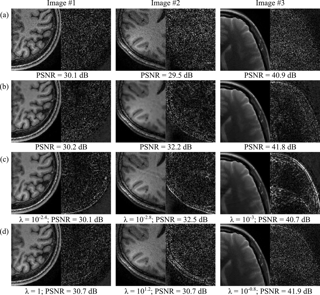
To study the potential for eliminating the requirement of estimating Λ from an additional noise-only acquisition, which requires additional time, the performance comparisons for moderate levels of uniform undersampling shown in Figure 4 are repeated for the slices of the three human datasets used previously, substituting the identity matrix for the measured noise covariance matrices. This approximation affects the coil combination weights, reweighting both the GRAPPA fidelity term of the DESIGN algorithm and the contributions of the reconstructed coil images to the combined image.

Figure 4.

Performance comparisons with R = 10.5, 10.5, and 12.4 uniform undersampling, for these three datasets, respectively. For the representative slices from each dataset, the magnitude and difference images of a representative region are shown, along with PSNR, for (a) GRAPPA, (b) GRAPPA with multichannel adaptive local Wiener-filter-based denoising, (c) L₁ SPIR-iT, and (d) DESIGN denoising. The PSNR-optimal choices of λ are shown for both L₁ SPIR-iT and DESIGN. Note that L₁ SPIR-iT is limited here by uniform undersampling.

Noise amplification and geometry factors

Geometry factors (g-factors) describe the noise amplification of a reconstruction method due to the geometry of the coils beyond the factor of √R loss of SNR due to undersampling k-space (2). For a linear algorithm like GRAPPA or SENSE, the noise amplification should also be linear, so the g-factors only depend on the sampling pattern/acceleration factor. Also, the g-factors can be computed analytically for GRAPPA, as is done in (31). For nonlinear algorithms, the SNR loss depends on the input noise level, so g-factors are valid only in a small range around that noise level. Note that while the PSNR is sensitive to most sources of error, including blurring and aliasing, g-factors are only indicative of noise amplification in the reconstruction. To compute the g-factors for GRAPPA, GRAPPA with multichannel adaptive Wiener filter-based denoising, L₁ SPIR-iT, and DESIGN, 400 Monte Carlo trials are used. The noise amplifications from each simulation are averaged, and the resulting values are combined across coils using the coil combination weights used to form the combined image. The parameters for each of the reconstruction algorithms are identical to those used in the preceding performance evaluations. In each trial, zero-mean additive white complex-valued Gaussian noise is added to the k-space data before performing reconstructions; the noise covariance Λ_AWGN is chosen to be the same as the noise covariance matrix Λ observed for the acquisition. This method for computing g-factors is described in (32).

Oversmoothing and loss of contrast

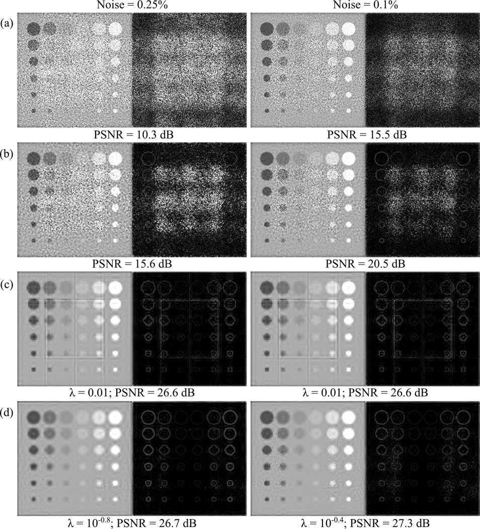
When denoising images, one must be careful not to oversmooth, as the reduction of contrast or resolution can hide important features. To explore the impact of DESIGN denoising on tissue contrast, a synthetic 32-channel contrast phantom (based on the phantom described in (33)) is generated, complex Gaussian noise is added, and the various reconstruction and denoising methods are compared on R = 12.1 uniform undersampled data from this phantom using the noise-free magnitude image as ground truth. This experiment is carried out for noise with 0.25% and 0.1% standard deviation (before amplification due to undersampling), to depict the extent of contrast loss at different noise levels. Parameter sweeps for λ are carried out for both DESIGN and L₁ SPIR-iT in each experiment.

Results

Several experiments are performed exploring design choices and comparing DESIGN to existing methods.

Optimizing the tuning parameter

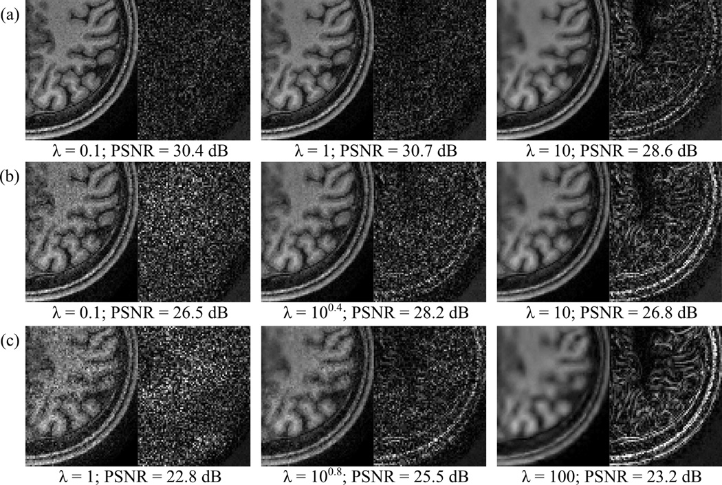
For DESIGN, the optimal choice of λ is expected to increase with R since the noise amplification due to GRAPPA and undersampling worsens with greater acceleration. In Figure 2, a representative region in DESIGN reconstructions of a slice of the first T₁-weighted MPRAGE dataset depict the trend in denoising and oversmoothing as λ increases, with optimal values of λ generally increasing at higher accelerations. The noise present in the leftmost column and the oversmoothing in the rightmost column together demonstrate the significance of tuning parameter selection in obtaining desirable results.

Figure 2.

DESIGN denoising results and difference images as λ increases, for the ℓ₁ norm with (a) R = 8.7, (b) R = 10.5, and (c) R = 12.0 uniform undersampling, all with the four-level ‘9-7’ DWT. The value of λ increases from left to right, and the results for the PSNR-optimal choice of λ for this dataset is shown in the center column. When λ is small, DESIGN resembles GRAPPA, and as λ increases, denoising and smoothing affect the result more noticeably. At high acceleration, these results suggest choosing a value of λ that denoises without excessive blurring becomes more challenging.

Performance comparisons

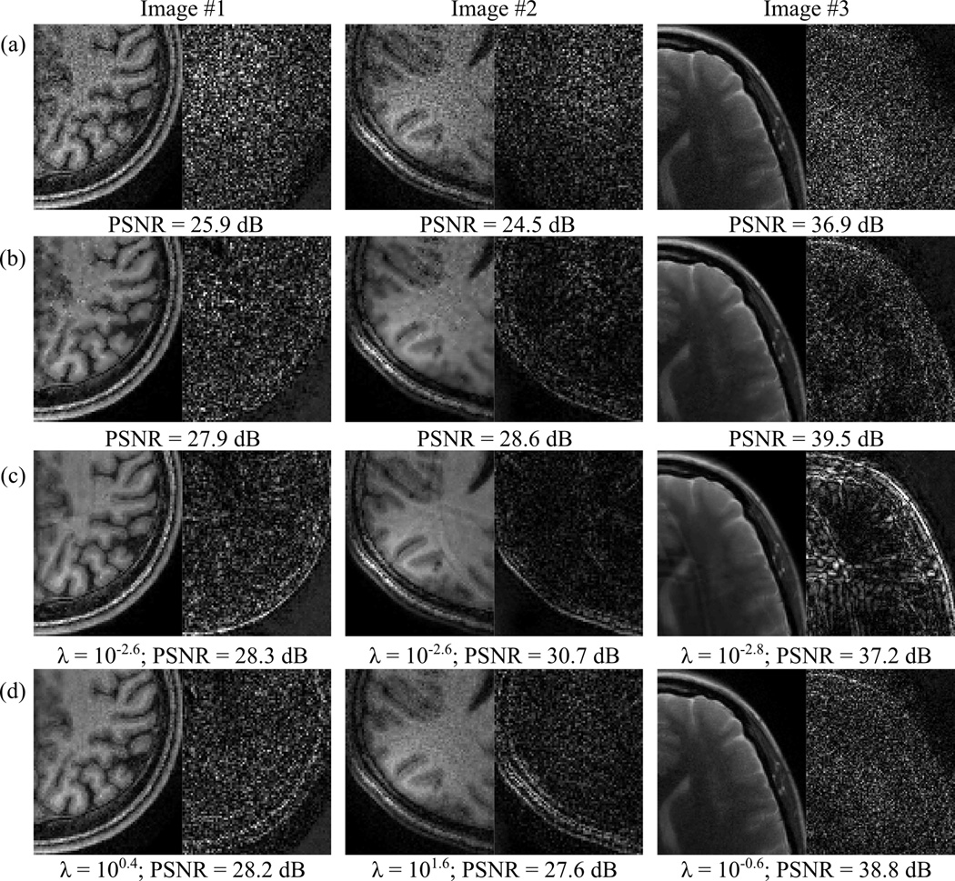
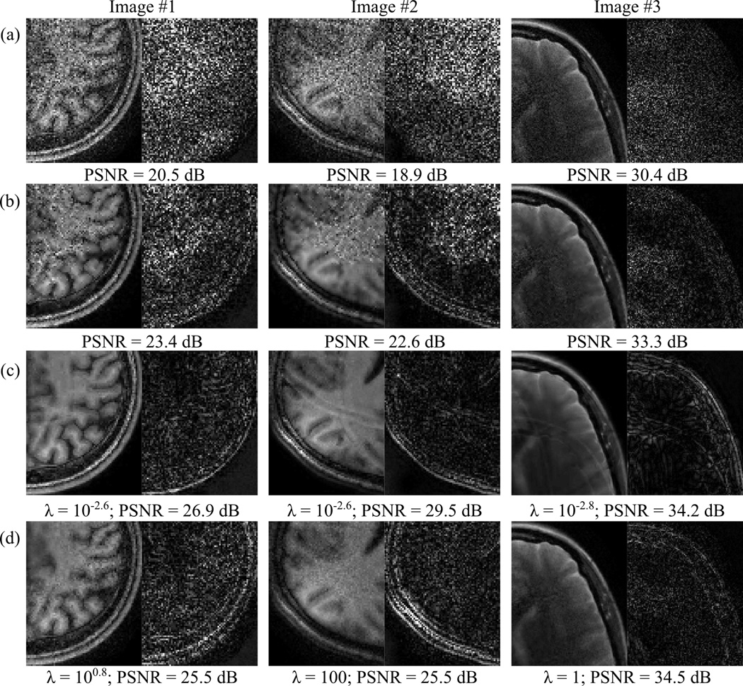
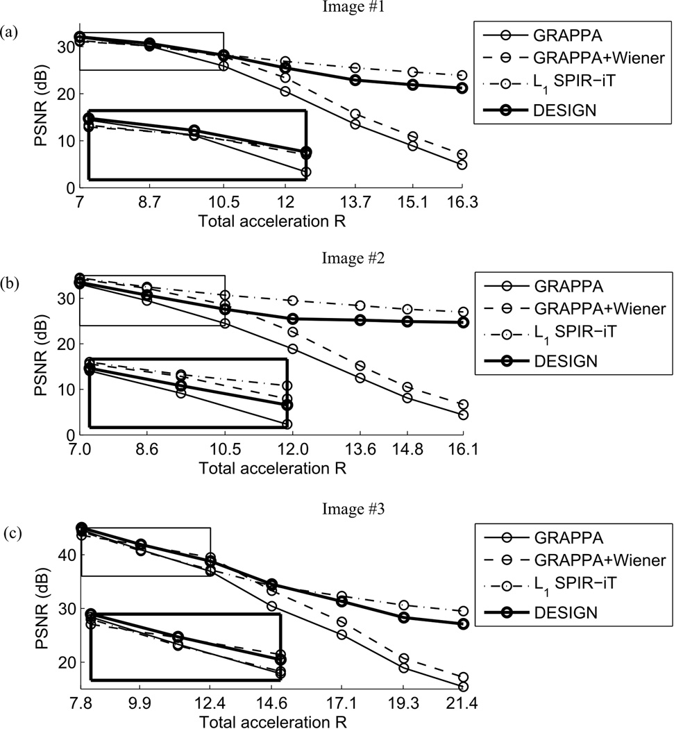
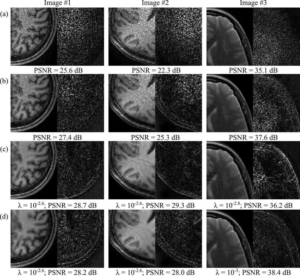
Results and difference images using GRAPPA, GRAPPA with multichannel adaptive local Wiener filter-based denoising, L₁ SPIR-iT, and DESIGN denoising are shown for representative slices of all three datasets in Figures 3–5 for increasing levels of uniform undersampling (see the figures for the total accelerations R of the three datasets), respectively. The magnitude image PSNR values for these different reconstruction methods are plotted as a function of R in Figure 6 for each of these images, over a broad range of total accelerations.

Figure 3.

Performance comparisons with R = 8.7, 8.6, and 9.9 uniform undersampling, respectively for these three datasets. For the representative slices from each dataset, the magnitude and difference images of a representative region are shown, along with PSNR, for (a) GRAPPA, (b) GRAPPA with multichannel adaptive local Wiener-filter-based denoising, (c) L₁ SPIR-iT, and (d) DESIGN denoising. The PSNR-optimal choices of λ are shown for both L₁ SPIR-iT and DESIGN. Note that L₁ SPIR-iT is limited here by uniform undersampling.

Figure 5.

Performance comparisons with R = 12, 12.1, and 14.6 uniform undersampling, respectively for these three datasets. For the representative slices from each dataset, the magnitude and difference images of a representative region are shown, along with PSNR, for (a) GRAPPA, (b) GRAPPA with multichannel adaptive local Wiener-filter-based denoising, (c) L₁ SPIR-iT, and (d) DESIGN denoising. The PSNR-optimal choices of λ are shown for both L₁ SPIR-iT and DESIGN. Note that L₁ SPIR-iT is limited here by uniform undersampling.

Figure 6.

Magnitude image PSNRs plotted vs. total acceleration R for representative slices of (a–b) two T₁-weighted MPRAGE datasets and (c) the T₂-weighted TSE dataset for GRAPPA, GRAPPA with multichannel adaptive local Wiener filter-based denoising, L₁ SPIR-iT, and DESIGN denoising. The inset regions display the PSNR trends for smaller R, where the methods’ performances are more similar. Note that L₁ SPIR-iT is limited here by uniform undersampling. For a given acceleration, the tuning parameter is determined for each dataset individually.

Several trends are evident from the images and plots. First, the noise power in the GRAPPA result increases significantly as R increases. As expected, the PSNR gain from denoising is more evident at higher accelerations. In addition, the noise amplification in L₁ SPIR-iT appears to increase far more slowly than with GRAPPA, so using the SPIR-iT parallel imaging result in place of the GRAPPA result may yield improved performance at high accelerations with only the additional computational cost up front to compute the SPIR-iT result. However, unlike GRAPPA, the L₁ SPIR-iT result appears far worse at un-aliasing without the help of random undersampling, as coherent aliasing is clearly visible in magnitude and difference images for the last two datasets in Figures 4 and 5. PSNR is insensitive to this aliasing since the effects are localized in the image. Blotches are clearly visible in the multichannel Wiener filter-denoised results; both L₁ SPIR-iT and DESIGN denoising produce more consistent images. The multichannel Wiener filter also appears in Figure 5 to hit its limit in denoising capability at very high accelerations. Finally, the evidence of similar levels of improvement from denoising using DESIGN over GRAPPA alone in each of the three datasets supports the broad applicability of the proposed method, at least for anatomical brain images.

Eliminating noise covariance estimation

Using the identity matrix in place of the measured noise covariance matrix, DESIGN is compared for moderately undersampled data against GRAPPA, GRAPPA with multichannel Wiener filter denoising, and L₁ SPIR-iT in Figure 7 as is done in the previous performance comparisons. The ability of DESIGN to improve upon the GRAPPA reconstructions for these three datasets appears hampered by using an identity matrix in place of the measured noise covariance matrix. In most cases, the images denoised with DESIGN still appear preferable to both GRAPPA alone or with multichannel Wiener filtering, reducing noise and producing few artifacts. Thus, if the measured noise covariance matrix is not available, the DESIGN method may still be used, to suboptimal results.

Figure 7.

Performance comparisons with R = 10.5, 10.5, and 12.4 uniform undersampling, for these three datasets, respectively, repeated using the identity matrix in place of the measured noise covariance. For the representative slices from each dataset, the magnitude and difference images of a representative region are shown, along with PSNR, for (a) GRAPPA, (b) GRAPPA with multichannel adaptive local Wiener-filter-based denoising, (c) L₁ SPIR-iT, and (d) DESIGN denoising. The choices of λ were established based on coarse, then fine, parameter sweeps for each dataset independently.

Noise amplification

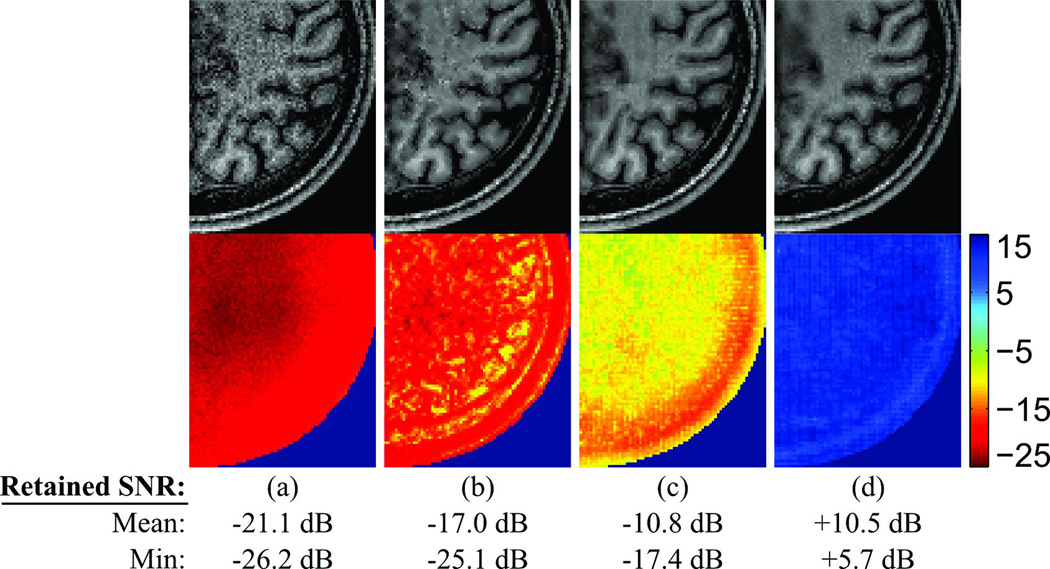
To further understand the denoising capabilities of DESIGN, the retained SNR (1/√R/g-factors) is shown for the first dataset with Λ_AWGN = Λ in Figure 8. GRAPPA, multichannel adaptive Wiener filter-based denoising, L₁ SPIR-iT, and DESIGN denoising are displayed below the reconstructed images reproduced from Figure 4, using exactly the same parameters as in the preceding performance comparisons, for R = 10.5. The substantially lower noise amplification present in the DESIGN result confirms the noise suppression from regularizing the GRAPPA result with sparsity; the noise suppression from DESIGN far exceeds that of the conventional denoising method based on multichannel local Wiener filtering. Due to the nonlinearity of the DESIGN algorithm, these results would be expected to change when the added noise power described by Λ_AWGN is varied. The present implementation of L₁ SPIR-iT does not appear to mitigate noise amplification nearly as much as DESIGN does for this acceleration factor. Thus, DESIGN may be combined with L₁ SPIR-iT in situations when noise suppression is a priority. More study is needed to understand this apparent advantage.

Figure 8.

The retained SNR in dB is compared across (a) GRAPPA, (b) GRAPPA with multichannel adaptive local Wiener filter-based denoising, (c) L₁ SPIR-iT, and (d) DESIGN denoising using the first dataset and the pseudo-multiple replica method with 400 Monte Carlo trials, for the four-level ‘9-7’ DWT with R = 10.5 uniform undersampling. The mean and minimum retained SNR correspond to the average and minimum gain/attenuation over the image, excluding the region without signal. The corresponding magnitude images for these reconstructions from Figure 4 are shown above for reference. The retained SNR maps are plotted on the same color scale to facilitate comparison.

Contrast loss and oversmoothing

The apparent downside of denoising using a method like DESIGN is the smoothing or blurring that results from aggressively employing a sparsity-based penalty; this blurring can reduce both contrast and spatial resolution. To quantify the loss of contrast due to denoising, we process the synthetic contrast phantom at two different noise levels and identify the circular contrast regions lost in the noise in the reconstruction. Upon visual inspection, we observe from Figure 9 that despite many of the contrast regions being lost in the noise in the GRAPPA reconstructions for both noise levels, those contrast regions are visible in the denoised DESIGN result. At the 0.25% noise level, the contrast of the central circles in the bottom row diminishes from ±10% to ±8%. At the 0.1% noise level, the contrast decreases to ±9%. Thus, contrast degradation does not appear to be significant at these noise levels.

Figure 9.

Synthetic 32-channel contrast phantom, with 0.25% and 0.1% complex Gaussian noise added, R = 12.1 uniformly undersampled, and reconstructed using (a) GRAPPA, (b) GRAPPA with multichannel adaptive local Wiener filter-based denoising, (c) L₁ SPIR-iT, and (d) DESIGN denoising, with a four-level ‘9-7’ DWT sparsifying transform. The magnitude difference images shown and the PSNR are relative to the original noise-free synthetic image.

Discussion

The primary design choices left to the user involve selecting an appropriate sparsifying transform and choosing the value of the tuning parameter. Throughout this paper, we achieve reasonable results using a four-level ‘9-7’ DWT; although not specifically tuned for brain images, a different transform may be necessary to apply DESIGN successfully to other types of data. The first experiment depicts the effect of choosing different values for the tuning parameter λ on DESIGN. As the primary design choice left to the user, the tuning parameter may be selected via either a parameter sweep, as is done in this paper, or a method like cross-validation.

The images depicting the results of reconstruction using DESIGN demonstrate that the proposed method mitigates noise amplification due to both undersampling and GRAPPA, improving PSNR and supporting the notion of sparsity-enforcing regularization as an effective denoising method. However, improvements in PSNR, like mean-squared error, are not indicative of improved diagnostic quality, and care must be taken to avoid oversmoothing. The included visual comparisons suggest that the DESIGN denoising method may be beneficial at moderately high accelerations, especially at a field strength of 3 T with a receive coil array with 32 channels. In addition, despite the sparsity regularization component of the joint optimization method, the algorithm functions properly with uniform undersampling, relying on GRAPPA to mitigate the aliasing; this feature obviates the need to dramatically redesign pulse sequences used for acquisition; existing noisy GRAPPA reconstructions may be improved by post-processing with this method.

However, the oversmoothing observed at very high accelerations suggests that this method may not be suitable for generating diagnostically useful images with extreme undersampling. The results from simulations involving synthetic 1.5 T data (with SNR degraded by added noise and gray/white matter contrast reduced according to T₁ values from (34)) are depicted in supplemental Figure S1. The reduction in image quality across all methods suggests that the feasible range of acceleration with this method is not as great as for 3 T; similar degradation is probable when far fewer coil channels are available. In addition, fewer channels reduces the ability of GRAPPA to resolve aliasing at high accelerations, and residual aliasing may remain in images denoised using DESIGN, reducing the proposed method’s utility at high accelerations. Further study is required to understand the limits of DESIGN in terms of aliasing and SNR loss from using 12- or 16-channel systems, and lower acceleration factors may be necessary with such systems.

The analysis using a synthetic contrast phantom supports that although DESIGN blurs low-contrast elements slightly, the degradation is not significant. Analyses of effective resolution conducted using both synthetic (based on the phantom described in (33)) and real Siemens multipurpose resolution phantoms are depicted in supplemental Figures S2–S4. Although the reconstructed image quality varies significantly among methods, the effective resolutions estimated using the full width at half maximum (FWHM) of horizontal and vertical cuts of the 2-D point-spread function (PSF) are all on the order of one voxel. However, this analysis is limited to simple features and relatively low noise levels and does not predict the contrast or texture degradation or loss of resolution that would result with applying DESIGN to denoise human images acquired at high accelerations; such oversmoothing may hinder the isolation of small features or low-contrast regions. Further tests on images with pathologies are necessary before the effects of oversmoothing can be ascertained definitively.

DESIGN denoising exhibits several distinctive characteristics when compared to L₁ SPIR-iT, the state-of-the-art method for combining compressed sensing and parallel imaging. First, when random undersampling is not possible, GRAPPA, and hence DESIGN, is far more effective at mitigating coherent aliasing than the underlying SPIR-iT approach; these artifacts are clear in several instances at high accelerations. Furthermore, according to the retained SNR maps, DESIGN is much more effective at denoising than L₁ SPIR-iT, ignoring the uniform sampling constraint. Moreover, not having to convolve the SPIR-iT (or GRAPPA) kernel with the k-space data in every iteration simplifies the implementation of the algorithm. In situations where random undersampling is used, DESIGN can denoise the L₁ SPIR-iT result, mitigating SNR loss at high accelerations.

In conclusion, the proposed method successfully combines GRAPPA and sparsity-based denoising. Adjusting the framework to accommodate non-uniform or non-Cartesian sampling patterns, using SPIR-iT or another non-uniform GRAPPA-like operator, and/or gridding techniques, would enable applicability to a greater number of acquisition schemes, including radial and spiral trajectories. In addition, the proposed algorithm can benefit greatly from implementation on a GPU, since the dominant computational operations (FFT and DWT) are all highly parallelizable. Such an implementation would enable cost-effective real-world application on clinical scanners. Further work includes testing DESIGN denoising on a variety of other types of MR images, carefully examining the effect of denoising on low-contrast anomalies like small tumors or lesions, and exploring more sophisticated sparsifying transforms or penalty functions suggested by a Bayesian analysis of the image denoising problem.

Supplementary Material

Supp Fig S1

Figure S1: Performance comparison with R = 10.5 uniform undersampling for the second dataset, with contrast reduced and complex Gaussian noise added to simulate the effects of lower T₁ and reduced SNR at 1.5 T, as shown in (a). The magnitude and difference images of a representative region are shown, along with PSNR, for (b) GRAPPA, (c) GRAPPA with multichannel adaptive local Wiener-filter-based denoising, (d) L₁ SPIR-iT, and (e) DESIGN denoising. The choices of λ were established based on coarse, then fine, parameter sweeps specifically for this dataset.

Supp Fig S2

Figure S2: Synthetic 32-channel resolution phantom, with added complex Gaussian noise (noise level = 1%), and regions A and B designed to measure horizontal and vertical resolution, respectively, is R = 12.1 uniformly undersampled, and reconstructed using (a) GRAPPA, (b) GRAPPA with multichannel adaptive local Wiener filter-based denoising, (c) L₁ SPIR-iT, and (d) DESIGN denoising, with a four-level ‘9-7’ DWT sparsifying transform. The magnitude point spread functions (PSFs) estimated for regions A and B are shown, a horizontal cut for region A, and a vertical cut for region B. Each reported horizontal and vertical resolution is based on the full width half maximum (FWHM) of the corresponding cut of PSF curve.

Supp Fig S3

Figure S3: Synthetic 32-channel resolution phantom, with added complex Gaussian noise (noise level = 0.25%), and regions A and B designed to measure horizontal and vertical resolution, respectively, is R = 12.1 uniformly undersampled, and reconstructed using (a) GRAPPA, (b) GRAPPA with multichannel adaptive local Wiener filter-based denoising, (c) L₁ SPIR-iT, and (d) DESIGN denoising, with a four-level ‘9-7’ DWT sparsifying transform. The magnitude point spread functions (PSFs) estimated for regions A and B are shown, a horizontal cut for region A, and a vertical cut for region B. Each reported horizontal and vertical resolution is based on the full width half maximum (FWHM) of the corresponding cut of PSF curve.

Supp Fig S4

Figure S4: Slice of (a) multipurpose resolution phantom, with horizontal and vertical grid regions labeled A and B, respectively, R = 11.2 uniformly undersampled, and reconstructed using (b) GRAPPA, (c) GRAPPA with multichannel adaptive local Wiener filter-based denoising, (d) L₁ SPIR-iT (λ = 10^−1.6), and (e) DESIGN denoising (λ = 10^1.2), with a four-level ‘9-7’ DWT sparsifying transform. The full images (a–e) are cropped around the phantom to show detail. Regions A and B in each reconstructed image are shown below the whole- magnitude image PSNRs. The magnitude point spread functions (PSFs) estimated for regions A and B are shown, a horizontal cut for region A, and a vertical cut for region B. Each reported horizontal and vertical resolution is based on the full width half maximum (FWHM) of the corresponding cut of PSF curve.

List of Symbols

A

matrix uppercase “a”

b

vector lowercase “bee”

C

matrix uppercase “cee”

D

matrix uppercase “dee”

Δ

Greek matrix uppercase “delta”

ε

Greek lowercase “epsilon”

F

matrix uppercase “ef”

G

matrix uppercase “gee”

I

matrix uppercase “i"

K

matrix uppercase “kay”

ℓ

script lowercase “el”

Λ

Greek matrix uppercase “lambda”

λ

Greek lowercase “lambda”

Ψ

Greek matrix uppercase “Psi”

W

matrix uppercase “double u”

w

vector lowercase “double-u”

X

matrix uppercase “ex”

x

vector lowercase “ex”

Y

matrix uppercase “wye”

References

- 1.Griswold M, Jakob P, Heidemann R, Nittka M, Jellus V, Wang J, Kiefer B, Haase A. Generalized autocalibrating partially parallel acquisitions (GRAPPA) Magn Reson Med. 2002;47(6):1202–1210. doi: 10.1002/mrm.10171. [DOI] [PubMed] [Google Scholar]
- 2.Pruessmann K, Weiger M, Scheidegger M, Boesiger P. SENSE: sensitivity encoding for fast MRI. Magn Reson Med. 1999;42(5):952–962. [PubMed] [Google Scholar]
- 3.Sodickson D, Manning W. Simultaneous acquisition of spatial harmonics (SMASH): fast imaging with radiofrequency coil arrays. Magn Reson Med. 1997;38(4):591–603. doi: 10.1002/mrm.1910380414. [DOI] [PubMed] [Google Scholar]
- 4.Lustig M, Pauly J. SPIRiT: Iterative self-consistent parallel imaging reconstruction from arbitrary k-space. Magn Reson Med. 2010;64(2):457–471. doi: 10.1002/mrm.22428. [DOI] [PMC free article] [PubMed] [Google Scholar]
- 5.Lustig M, Donoho D, Pauly J. Sparse MRI: The application of compressed sensing for rapid MR imaging. Magn Reson Med. 2007;58(6):1182–1195. doi: 10.1002/mrm.21391. [DOI] [PubMed] [Google Scholar]
- 6.Candes E, Romberg J, Tao T. Robust uncertainty principles: Exact signal reconstruction from highly incomplete frequency information. IEEE Transactions on Information Theory. 2006:489–509. [Google Scholar]
- 7.Candes E, Romberg J. Quantitative robust uncertainty principles and optimally sparse decompositions. Foundations of Computational Mathematics. 2006:227–254. [Google Scholar]
- 8.Donoho D. Compressed sensing. IEEE Transactions on Information Theory. 2006:1289–1306. [Google Scholar]
- 9.Lustig M, Alley M, Vasanawala SS, Donoho DL, Pauly JM. L1 SPIR-IT: Autocalibrating Parallel Imaging Compressed Sensing. 17th Annual Meeting of ISMRM; Honolulu, HI, USA: ISMRM. 2009. p. 379. [Google Scholar]
- 10.Murphy M, Keutzer K, Vasanawala S, Lustig M. Clinically Feasible Reconstruction Time foRL1-SPIRiT Parallel Imaging and Compressed Sensing MRI. 18th Annual Meeting of ISMRM; Stockholm, Sweden: ISMRM. 2010. p. 4854. [Google Scholar]
- 11.Weller DS, Polimeni JR, Grady LJ, Wald LL, Adalsteinsson E, Goyal VK. Combining nonconvex compressed sensing and GRAPPA using the nullspace method. 18th Annual Meeting of ISMRM; Stockholm, Sweden: ISMRM. 2010. p. 4880. [Google Scholar]
- 12.Fischer A, Seiberlich N, Blaimer M, Jakob PM, Breuer FA, Griswold MA. A Combination of Nonconvex Compressed Sensing and GRAPPA (CS-GRAPPA). 17th Annual Meeting of ISMRM; Honolulu, HI, USA: ISMRM. 2009. p. 2813. [Google Scholar]
- 13.Liang D, Liu B, Wang J, Ying L. Accelerating SENSE using compressed sensing. Magn Reson Med. 2009;62(6):1574–1584. doi: 10.1002/mrm.22161. [DOI] [PubMed] [Google Scholar]
- 14.Brau AC, Beatty PJ, Skare S, Bammer R. Comparison of reconstruction accuracy and efficiency among autocalibrating data-driven parallel imaging methods. Magn Reson Med. 2008;59(2):382–395. doi: 10.1002/mrm.21481. [DOI] [PMC free article] [PubMed] [Google Scholar]
- 15.Grady LJ, Polimeni JR. Nullspace Compressed Sensing for Accelerated Imaging. 17th Annual Meeting of ISMRM; Honolulu, HI, USA: ISMRM. 2009. p. 2820. [Google Scholar]
- 16.Chartrand R. Exact reconstruction of sparse signals via nonconvex minimization. IEEE Signal Processing Letters. 2007:707–710. [Google Scholar]
- 17.Trzasko J, Manduca A. Highly Undersampled Magnetic Resonance Image Reconstruction via Homotopic l(0)-Minimization. IEEE Transactions on Medical Imaging. 2009:106–121. doi: 10.1109/TMI.2008.927346. [DOI] [PubMed] [Google Scholar]
- 18.Roemer P, Edelstein W, Hayes C, Souza S, Mueller O. The NMR phased array. Magn Reson Med. 1990;16(2):192–225. doi: 10.1002/mrm.1910160203. [DOI] [PubMed] [Google Scholar]
- 19.Holland P, Welsch R. Robust Regression Using Iteratively Re-Weighted Least-Squares. Communications in Statistics Part a-Theory and Methods. 1977:813–827. [Google Scholar]
- 20.Zelinski A, Goyal V, Adalsteinsson E. Simultaneously Sparse Solutions to Linear Inverse Problems with Multiple System Matrices and a Single Observation Vector. SIAM Journal on Scientific Computing. 2010:4533–4579. doi: 10.1137/080730822. [DOI] [PMC free article] [PubMed] [Google Scholar]
- 21.Fong DC-L, Saunders MA. LSMR: An iterative algorithm for sparse least-squares problems: Systems Optimization Laboratory. Stanford University. 2010 [Google Scholar]
- 22.Geman D, Reynolds G. Constrained Restoration and the Recovery of Discontinuities. IEEE Transactions on Pattern Analysis and Machine Intelligence. 1992;14(3):367–383. [Google Scholar]
- 23.Geman D, Yang C. Nonlinear image recovery with half-quadratic regularization. IEEE Transactions on Image Processing. 1995;4(7):932–946. doi: 10.1109/83.392335. [DOI] [PubMed] [Google Scholar]
- 24.Nikolova M, Chan RH. The equivalence of half-quadratic minimization and the gradient linearization iteration. IEEE Transactions on Image Processing. 2007;16(6):1623–1627. doi: 10.1109/tip.2007.896622. [DOI] [PubMed] [Google Scholar]
- 25.Candes E, Demanet L, Donoho D, Ying L. Fast discrete curvelet transforms. Multiscale Modeling & Simulation. 2006:861–899. [Google Scholar]
- 26.Do M, Vetterli M. The contourlet transform: An efficient directional multiresolution image representation. IEEE Transactions on Image Processing. 2005:2091–2106. doi: 10.1109/tip.2005.859376. [DOI] [PubMed] [Google Scholar]
- 27.Easley G, Labate D, Lim W. Sparse directional image representations using the discrete shearlet transform. Applied and Computational Harmonic Analysis. 2008:25–46. [Google Scholar]
- 28.Tibshirani R. Regression shrinkage and selection via the Lasso. Journal of the Royal Statistical Society Series B-Methodological. 1996:267–288. [Google Scholar]
- 29.Lin FH, Kwong KK, Belliveau JW, Wald LL. Parallel imaging reconstruction using automatic regularization. Magn Reson Med. 2004;51(3):559–567. doi: 10.1002/mrm.10718. [DOI] [PubMed] [Google Scholar]
- 30.Donoho D, Johnstone I. Ideal Spatial Adaptation by Wavelet Shrinkage. Biometrika. 1994;81(3):425–455. [Google Scholar]
- 31.Breuer F, Kannengiesser S, Blaimer M, Seiberlich N, Jakob P, Griswold M. General formulation for quantitative G-factor calculation in GRAPPA reconstructions. Magn Reson Med. 2009;62(3):739–746. doi: 10.1002/mrm.22066. [DOI] [PubMed] [Google Scholar]
- 32.Robson PM, Grant AK, Madhuranthakam AJ, Lattanzi R, Sodickson DK, McKenzie CA. Comprehensive quantification of signal-to-noise ratio and g-factor for image-based and k-space-based parallel imaging reconstructions. Magn Reson Med. 2008;60(4):895–907. doi: 10.1002/mrm.21728. [DOI] [PMC free article] [PubMed] [Google Scholar]
- 33.Smith DS, Welch EB. Non-Sparse Phantom for Compressed Sensing MRI Reconstruction. 19th Annual Meeting of ISMRM; Montreal, Canada: ISMRM. 2011. p. 2845. [Google Scholar]
- 34.Ethofer T, Mader I, Seeger U, Helms G, Erb M, Grodd W, Ludolph A, Klose U. Comparison of longitudinal metabolite relaxation times in different regions of the human brain at 1.5 and 3 Tesla. Magn Reson Med. 2003;50(6):1296–1301. doi: 10.1002/mrm.10640. [DOI] [PubMed] [Google Scholar]
Associated Data
This section collects any data citations, data availability statements, or supplementary materials included in this article.
Supplementary Materials