Decision value computation in DLPFC and VMPFC adjusts to the available decision time

Abstract

It is increasingly clear that simple decisions are made by computing decision values (DV) for the options under consideration, and then comparing these values to make a choice. Computational models of this process suggest that it involves the accumulation of information over time, but little is know about the temporal course of valuation in the brain. To examine this, we manipulated the available decision time and observed the consequences in the brain and behavioral correlates of choice. Participants were scanned with functional magnetic resonance imaging while they chose to eat or not eat basic food items, in two conditions differing in the amount of time provided for choice. After identifying valuation-related regions with unbiased whole-brain general linear models, we analyzed two regions of interest: ventromedial prefrontal cortex (VMPFC) and dorsolateral prefrontal cortex (DLPFC). Finite impulse response models of the upsampled estimated neural activity from those regions allowed us to examine the onset, duration, and termination of decision value signals, and to compare across regions. We found evidence for the immediate onset of value computation in both regions, but an extended duration with longer decision time. However, this was not accompanied by behavioral changes in either the accuracy or determinants of choice. Finally there was modest evidence that DLPFC computation correlated with, but lagged behind VMPFC computation, suggesting the sharing of information across these regions. These findings have important implications for models of decision value computation and choice.

INTRODUCTION

There is a growing consensus that the brain makes simple decisions by assigning a decision value (DV) to the options under consideration, and then comparing these values to make a choice (Rangel and Hare, 2010; Padoa-Schioppa, 2011; Rushworth et al., 2011). In this framework, understanding the DVs’ properties is critical, because they affect the choices that are eventually made. For example, if DVs are noisy when decisions are made under time pressure, then so are choices (Milosavljevic et al., 2010; Milosavljevic et al., 2011).

A considerable amount has been learned about the computational and neurobiological properties of the DV signals. A large number of studies, utilizing different species and techniques, consistently link activity in the ventromedial prefrontal cortex (VMPFC) with the computation of DVs at the time of choice (Rangel and Hare, 2010; Wallis and Kennerley, 2010; Padoa-Schioppa, 2011). Activity in dorsolateral prefrontal cortex (DLPFC) also frequently correlates with DVs, though less consistently (Kable and Glimcher, 2007; Plassmann et al., 2007; Litt et al., 2010; Plassmann et al., 2010). In several decision tasks involving self-control, the DV signals in VMPFC seem to be constructed using inputs from DLPFC areas that do not encode for DVs themselves (Hare et al., 2009; Figner et al., 2010; Baumgartner et al., 2011; Hare et al., 2011a). Finally, recent studies have shown that similar areas of VMPFC and DLPFC are part of the network involved in comparing DVs to make a choice (Basten et al., 2010; Hare et al., 2011b).

Although these findings have established the critical role of VMPFC and DLPFC in the computation of DVs at the time of choice, the nature of the DV signals encoded, as well as how they relate to choices, have not been systematically investigated. Four questions are of particular interest. First, does the available decision time affect the duration and quality of decision value signals in VMPFC and DLPFC? Second, do the changes in the DV signals have an effect on the quality of choices? Third, are there differences between regions in how decision value signals evolve over time within decision episodes? And fourth, are there differences in the stimulus information that is used to compute the decision value signals in VMPFC and DLPFC (e.g., taste versus health attributes for foods)?

The answers to these questions are important because they have direct bearing on the properties and quality of the decision-making circuitry, and how it is affected by environmental variables such as time pressure or distraction. For example, it is not known if the brain keeps refining its estimates of DV if given extra decision time, or if stops computing them as soon as the estimate is satisfactory, even if extra time remains (Kiani et al., 2008). In the former case extra decision time could have a positive impact on the quality of choices, but in the latter it is just wasted time. The relationship between the two DV signals is also poorly understood. Some have argued that VMPFC signals serve as precursors to DLPFC signals, which eventually drive choices (Wallis and Miller, 2003). In contrast, in other decision paradigms the influence appears to go in the other direction (Hare et al., 2009; Baumgartner et al., 2011).

Here we describe the results of an fMRI experiment in which participants were asked to make consumption decisions about snack foods under two externally controlled decision speeds: fast (1s) and slow (4s) choices. The results of the experiment allow us to systematically test specific hypotheses associated with each of these three questions (see Results section for details).

METHODS

Participants

Twenty-eight participants completed both sessions of the study (8 females, mean age [SD] = 22.4 [0.6] years). Of these, six participants were excluded from data analysis: one due to scanner malfunction during the study, two for excess head motion during scanning (total translation greater than 3mm or total rotation greater than 2.45 degrees in any single volume), and three due to highly atypical behavioral responses that suggested that they were not taking the task seriously (i.e. responding without considering the stimuli, as evidenced by having identical consecutive responses in more than 50% of trials). Twenty-two participants were used in the analyses (6 females, mean age [SD] = 22.6 [0.6] years). All participants gave written informed consent, and all procedures were approved by Caltech’s Institutional Review Board.

Task

The experiment took place over two sessions, separated by one to four days. On day 1, we collected basic subject specific information about the stimuli used in the experiment. On day 2, participants performed an in-scanner choice task.

Day 1

For the first behavior-only session, participants were asked to fast for at least four hours prior to the experiment. Participation in the task was contingent on signing a statement affirming that they had not eaten or drunk anything except water for the past 4 hours, and reporting no food allergies or intolerances. During this session, participants rated 249 color images of different appetitive and aversive snack food items (e.g. Kit-Kat bar, apple slices, Spam; see Supplementary Materials for a complete list) on three different 5-point scales: Liking (Strongly Dislike to Strongly Like), Tastiness (Very Bad to Very Good), and Healthiness (Very Unhealthy to Very Healthy). Ratings were blocked, so that all ratings of a given type were completed before moving onto ratings of a different type. Liking ratings for all foods were assessed first, randomly followed by ratings of Healthiness and Tastiness (order counterbalanced across participants).

On every trial, participants were shown one of the food items for 1s, with a white box around it, during which they could not respond. Immediately after the box disappeared, participants entered ratings at their own pace. Their response was followed by a 1s feedback screen displaying the rating they had selected. Trials were separated by a uniform random 1–3s screen with a centered fixation cross. Ratings scales were displayed and explained before each block, and the left-right order of each rating type was separately randomized across participants.

Day 2

The same 4-hour fasting and screening criteria were implemented in the second session. After detailed instruction, participants performed a simple choice task in the scanner. Every trial they were shown one food item and had to decide whether they wanted to eat it at the end of the experiment. They indicated their choices using a 4-point scale (Strong Yes, Yes, No, Strong No; left/right ordering randomized across participants), which allowed us to measure simultaneously their decisions and the strength of their preferences. Participants cared about their decisions because they knew that they would have to stay in the lab for 20 minutes at the end of the experiment, and that the only thing that they would be allowed to eat would be based on their decisions. Specifically, one trial was randomly selected and participants were required to eat that food item if their response was “Strong Yes” or “Yes”, and were not allowed to eat it otherwise.

The structure of the decision task was similar to the ratings task (Figure 1). The only differences were as follows: 1) the initial “viewing period” of the foods now lasted either 1s (Short condition) or 4s (Long condition), 2) participants had to indicate their decision within 1s of the beginning of the response period or the trial aborted, and 3) the intertrial intervals were drawn uniformly from 1–6s. To maintain the spacing across trials, the unused fraction of the response period was added to the intertrial interval. Stimuli were divided between the Short and Long conditions based on each participant’s liking ratings in the behavioral session, to equate the distribution of Liking ratings across conditions. Conditions were blocked (25 trials/block), and block order was randomized subject to the constraint that there were two blocks of each type (Short; Long) during each functional scan. Blocks were preceded with an instruction cue indicating the duration of the viewing period in the upcoming block of trials: (shown for 5s, followed by a 1s fixation cross) informing participants about the upcoming condition. There were 200 trials in each condition (400 trials total; 8 blocks of each trial type, 16 blocks total). See the Supplementary Materials for details on how foods were distributed between conditions.

Figure 1.

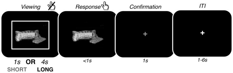
Scanner choice task. On each trial, a color image of a food item appeared surrounded by a white box for either 1s (Short condition) or 4s (Long condition). During this time participants were not allowed to enter a response. Afterwards the white box disappeared and participants had up to 1s to enter their choice on a 4-point scale (Strong Yes, Yes, No, or Strong No). Immediately after response, a 1s confirmation screen appeared with a green fixation cross. Trials were separated by an inter-trial interval of 1–6s rand duration.

fMRI: Data collection

Scanning was performed at the Caltech Brain Imaging Center with a Siemens 3T TIM-Trio full body scanner and a Siemens 32-channel phased array head coil. High-resolution anatomical images were acquired using a T1-weighted protocol (FOV=256, 176 slices, 1x1x1mm). Functional imaging used a gradient echo EPI sequence (TR=2530ms, TE=30ms, FOV=192, anterior to posterior phase encoding, ascending slice acquisition), acquiring 4 functional runs of 334 volumes, each with 40 oblique axial slices aligned 30° off the AC-PC plane (to improve signal in the orbitofrontal cortex (Deichmann et al., 2003)), 3mm isometric voxels, and a 0.3mm between-slice gap.

fMRI: Preprocessing

Two volumes were discarded before the beginning of data collection in each run to allow for equilibration of the magnetic field. Data were preprocessed with SPM8 software (Statistical Parametric Mapping 8, Wellcome Trust Center for Neuroimaging; http://www.fil.ion.ucl.ac.uk/spm/), including slice time correction, realignment (motion correction), and spatial smoothing (isotropic 6mm FWHM Gaussian kernel). Functional runs were coregistered and normalized to the standard Montreal Neurological Institute EPI template. Data were high-pass filtered prior to analysis (cutoff = 128s).

fMRI: Whole brain analyses

Analysis was performed with SPM8 and custom MATLAB scripts (Mathworks, Natick, MA, USA). Individual level whole brain general linear models (GLMs) with AR(1) and SPM8’s standard hemodynamic response function were estimated in three steps. First, we estimated the model separately for each individual. Second, we calculated contrast statistics at the individual level. Third, we computed second-level statistics by carrying out one-sample t tests on the single-subject contrast coefficients.

GLM 1

This model contained the following three regressors of interest: R1) Regressor for initial stimulus presentation, in the form of a boxcar function that ran from image onset to response, pooling across both the Short and Long conditions; R2) Decision Value regressor, created by modulating R1 by the subject’s decision value on each trial (Strong No= −1.5, No = −0.5, Yes = 0.5, Strong Yes = 1.5); and R3) Response time regressor, in the form of a stick function at the time of the response.

GLM 2

The second GLM consisted of the following regressors of interest: R1) Regressor for Short trials only, in the form of a boxcar from image onset to response; R2) Tastiness Rating regressor for Short trials, created by modulating R1 by the Tastiness rating (Very Bad = −2 to Very Good = 2); R3) Healthiness Rating regressor for Short trials, created by modulating R1 by the Healthiness rating (Very Unhealthy = −2 to Very Healthy = 2); R4) Regressor for Long trials only, in the form of a boxcar from image onset to response; R5) Tastiness Rating modulated regressor for Long trials; R6) Healthiness Rating modulated regressor for Long trials; R7) Indicator for response in Short trials; and R8) Indicator for response in Long trials.

In addition, both GLMS also included the following nuisance regressors: estimates of motion from preprocessing, and separately for each condition, boxcars for the pre-block instruction cues (5s), transient predictors for item presentation when participants failed to respond, transient predictors for item presentation when participants responded too early, and transient predictors for the response itself when participants responded too early.

In our whole-brain analysis we localize activity for the contrasts of interest using the a liberal but common statistical threshold: p < 0.001 uncorrected with a 5 contiguous voxel extent threshold. We chose this criterion to give the best chance of identifying the desired regions of interest (ROIs) for further investigation..

fMRI: ROI definition

Most analyses in the paper examined the patterns of activation in two pre-specified ROIs: the VMPFC and left DLPFC regions exhibiting BOLD responses modulated by DVs (R2) in GLM 1. The resulting functionally specified ROIs are depicted in Figure 2. The VMPFC ROI consisted of all voxels significant in this contrast at p < 0.00001, uncorrected (78 voxels). This stringent threshold was necessary to prevent the inclusion of voxels from other distinct areas of the brain (e.g. ventral striatum, cingulate). The DLPFC ROI consisted of all voxels significant at p < 0.001, uncorrected (7 voxels). After identifying regions of interest (ROIs) in whole-brain analyses, the responses within these regions was investigated in two ways: 1) raw BOLD data was extracted from these ROIs for deconvolved (neural signal) finite impulse response (FIR) analyses, and 2) mean parameters within the ROIs from the whole-brain GLM 2 (Taste & Health) were extracted for use in conventional BOLD analyses.

Figure 2.

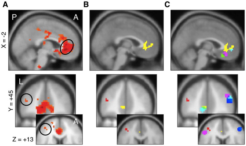
Whole-Brain localization of DV signals and ROIs. A) Areas in which BOLD responses during the initial period of stimulus presentation were positively modulated by decision values, regardless of condition (p < 0.001 unc, k = 5, see GLM 1). Hot colors indicate positive contrast values, cold colors indicate negative contrast values. The circles identify the VMPFC (top) and DLPFC (bottom) regions correlated with decision value. B) ROIs used in further analyses: VMPFC = yellow, DLPFC = red. C) Relationship between the ROIs and areas in VMPFC and DLPFC that have been shown elsewhere to correlate with DVs at the time of choice: Plassmann et al, 2010 (left DLPFC, purple), Plassmann et al, 2007 (right DLPFC, blue), McClure et al, 2004 (VMPFC, cyan), and Hare et al, 2007 (VMPFC, green).

fMRI: Neural Estimate Analyses

Although standard approaches often present analyses based on BOLD responses, hemodynamic responses are substantially delayed and prolonged relative to the neural signals that generated them. This means that analyses sensitive to small differences in timing (on the order of 1–3 seconds) can often be difficult to visualize or interpret using these approaches. To better address questions specific to the timing of value signals, we therefore turned to deconvolution methods designed to extract an estimated neural response (Gitelman et al., 2003). This deconvolution procedure offers the additional benefit of using a constrained set of HRF parameters rather than a single fixed HRF. This accounts for some of the differences that may arise between regions, lowering the risk of systematic bias, and increasing our ability to compare the ‘neural estimates’ across regions (see Supplementary Materials for comparable analyses performed on the non-deconvolved BOLD responses).

This analysis proceeded in the following steps.

First, for every voxel within an ROI, the raw BOLD signal at each TR was extracted, mean-corrected, and adjusted for motion using standard SPM tools.

Second, the resulting timecourses for each individual’s extracted data were then subjected to singular value decomposition, and the first eigenvariate (i.e. the first principal component of the raw time series from all voxels within the ROI) was used as the index of the regional response (Friston et al., 1996; O'Reilly et al., 2010; Mars et al., 2011a; Mars et al., 2011b). This technique captures the signal representing the greatest proportion of variance within the ROI (i.e. that which is most coherent across the voxels), making it less susceptible to noise from any given voxel, compared to a simple average (Friston et al., 1996; Gitelman et al., 2003).

Third, a “neural estimate” was constructed by deconvolving the BOLD timecourse with the formula for SPM8’s canonical hemodynamic response function (HRF) using standard SPM scripts employing a parametric empirical Bayes formulation (Gitelman et al., 2003). This deconvolution entailed assumptions common to all analyses using HRFs (including classic whole-brain general linear models), such as assumptions of HRF linearity, shape, and consistency across regions. As in any analyses requiring these or similar assumptions, any inferences are predicated on the accuracy of those assumptions.

Fourth, the ‘neural estimate’ resulting from this deconvolution was linearly interpolated (up-sampled) to a resolution of 1/16^th of a TR (0.158s). This fine temporal resolution is preferred in order to reduce the temporal blurring associated with rounding event onset times to the nearest data timepoint in the finite impulse response analyses described below.

Finally, we estimated finite impulse-response (FIR) models on these data for each individual, ROI, and scan session. In an FIR model, events of interest are modeled with multiple regressors, each estimating the signal at a single given timepoint relative to event onset. Note that because this technique estimates the signal at discrete timepoints, regressors must be similarly aligned, incurring temporal blurring proportional to the timecourse resolution. Events of interest were modeled with 19 sequential non-overlapping transient predictors in the Short (1s) condition (covering the three seconds from the onset of the image to the end of the trial), and 38 transient predictors in the Long (4s) condition (to cover the six seconds from image onset to the end of the trial). The resulting models included separate regressors for each response type (Strong Yes, Yes, No, and Strong No) and a session constant. After estimation, parameter estimates were averaged across the four scan sessions for each participant. Because the hemodynamic response was deconvolved from the ROI data, no hemodynamic lag is expected in the ‘neural estimates’. One participant was excluded from the FIR analyses because they never provided a Strong No response.

We report three different types of FIR analyses. First, we examine the instantaneous differences in the FIR estimates between Strong-Yes (SY) and Strong-No (SN) trials. This provides a measure of the instantaneous DV signal (i.e., the difference score increases as the neural responses associated with DV signals become more discriminating between SY and SN trials). Second, because computational models of choice behavior suggest that decisions result from the accumulation of information over time (Kiani et al., 2008; Ratcliff and McKoon, 2008; Kiani and Shadlen, 2009), we also looked at differences in the cumulative value signal. In particular, for any time t, let v(t) be the SY-SN difference score at that time. The cumulative value difference at time T is then given by the sum of all v(t) from t=0 to t=T. This analysis allows us to test if there are differences across conditions or regions in how the DV signals accumulate over time. Third, we examined differences in the timing of valuation by a) computing the time of the peak value computation (t at which SY-SN_t = max[SY-SN]), and b) computing the number of time-points we had to shift the Short SY-SN curve to best match the Long SY-SN curve, by minimizing the sum of the squared differences at the overlapping points (intuitively, the point at which the two curves were the most similar).

fMRI: BOLD ROI analyses

Using the VMPFC and DLPFC ROIs, we also conducted a standard analysis based on the BOLD signal. Using GLM 2, we extracted average beta coefficients for the weighting of Tastiness and Healthiness in the Short and Long conditions from each ROI for each subject and subjected them to a detailed analysis examining the influence of decision time on the neural representation of each attribute.

RESULTS

This section is organized as follows. First, we described the results of a whole brain analysis of the BOLD data designed to identify areas of VMPFC and DLPFC in which BOLD responses are correlated with DVs, for both experimental conditions. The results of this analysis are used to defined two functional ROIs, one for VMPFC and one for DLPFC, which are similar to those that have been identified in previous studies. Second, we carry out various ROI based analyses of the properties of the DV signals encoded in these two areas, which are used to systematically address the four questions posed in the introduction.

Whole brain analysis: Correlation with DVs during the evaluation period

We estimated a general linear model of brain responses in which activity during the entire evaluation period (i.e., from stimulus onset to response prompt, 1s in Short condition and 4s in Long condition) was modulated by DVs (see GLM 1 in Methods for details). DVs were measured using the 4-point response scale (Strong-No, No, Yes, Strong-Yes). Figure 2A depicts regions in which the BOLD responses were positively correlated with DVs, which as expected included areas of VMPFC and left DLPFC (see Table S1 in supplementary materials for full list of activations).

These results were used to functionally define ROIs in VMPFC and DLPFC, depicted in Figure 2B, that are used in all subsequent analyses. Note that their location aligned well with previous reports (Figure 2c; McClure et al., 2004; Plassmann et al., 2007; Hare et al., 2008; Plassmann et al., 2010) and that their definition was statistically independent of tests below that compare the two conditions, since GLM 1 imposes a common estimate for the DV regressor for both conditions.

Question 1: Does available decision time influence the timing of DV signals?

Our primary research question concerned whether the amount of available decision time influenced the timing of decision value computations in the brain (e.g., changing the onset, duration, or trajectory, as compared to the null hypothesis that time has no influence on these computations). Evidence for such changes would help to explain behavioral findings that time pressure can lead to less accurate choices (Milosavljevic et al., 2010; Milosavljevic et al., 2011) and might complement evidence from the perceptual literature that evidence accumulation begins immediately but continues only until a decision threshold is crossed, even if more time and information are available (Kiani et al., 2008; Kiani and Shadlen, 2009). This evidence suggests that we should observe changes in the timing of subjective decision value computation as a function of available decision time, although the precise nature of these changes could take several forms, three of which we test below.

We tested this hypothesis using extracted ‘neural estimates’ of value-related activity in VMPFC and DLPFC and finite impulse response (FIR) analyses that estimate neural responses in each ROI, time bin, and condition separately for each response type (Strong Yes, Yes, No, and Strong No). This combination of methods allows us to compare signals, without lag, across regions because it does not assume the same shape for the hemodynamic response in each area (see Methods for full details and justification. For analyses reported in the paper, we defined an index of the instantaneous DV signal in each time bin by the difference between the Strong-Yes (SY) and Strong-No (SN) responses (Figure 3A, B; see Figure S1 for separate SY, Y, N, and SN responses). The larger the SY-SN score (i.e. the more strongly items were differentiated based on value), the more value computation was taking place. Intuitively, an SY-SN difference score of zero at a given moment indicates no value computation at that time. As the SY-SN difference score becomes significantly different from zero, it indicates a stronger and more consistent representation of stimulus values.

Figure 3.

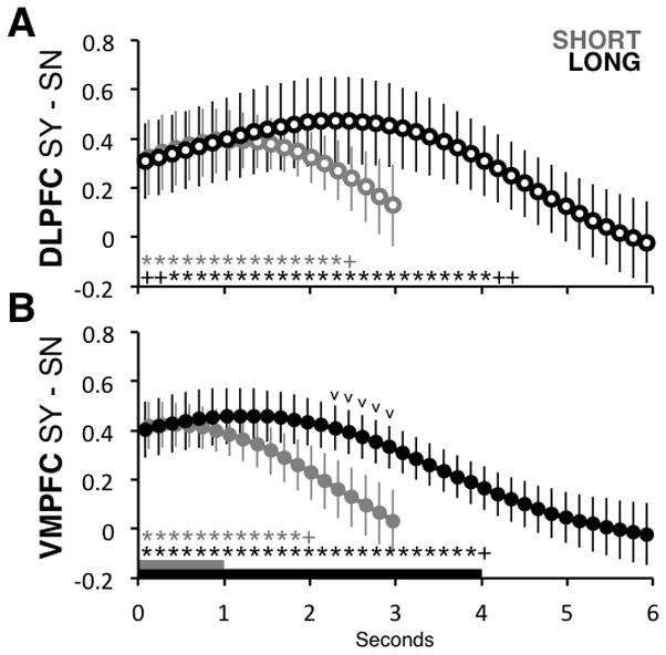
Instantaneous Neural Estimate Analyses. A) Estimate of the difference in activity levels in the DLPFC ROI between trials with Strong-Yes (SY) and Strong-No (SN) responses, for each time bin and condition. Gray and black bars at the bottom of the figure indicate the length of time the foods were initially shown in each condition. Gray or black asterisks indicate that the difference between SY and SN was significantly different from zero at p < 0.05 (pluses indicate marginally different at p < .1), based on a paired t-test computed across subjects. B) Analogous estimates for the VMPFC ROI. Black carets indicate a marginal difference between the estimates for the two conditions (p < 0.1, paired t-test). Error bars are standard error of the mean calculated across participants. See Methods and Results section for details on how the measures are computed. “a.u.” = arbitrary units.

We first tested for differences in onset of DV computations in Short vs. Long trials. We found that in both ROIs, the onset of value computation appeared to be immediate and of identical magnitude. In other words, the magnitude of the response during the first second was significantly above zero at all time points, and did not differ between Short and Long trials in either region (all timepoints n.s.).

We next compared differences in the duration of DV computation. This comparison revealed significantly longer DV computation in the Long condition, in both regions. In other words, whereas in the Short condition the DV signal becomes statistically indistinguishable from zero about two 2s after stimulus onset (DLPFC timepoint 15, 2.37s; VMPFC timepoint 12, 1.89s), in the Long condition the DV signal is present for nearly twice as long (DLPFC timepoint 26, 4.11s; VMPFC timepoint 25, 3.95s). Note that although the termination of computation aligns to the end of the viewing window in the Long condition, it extends a full second past this point in the Short condition. To test these observations of duration differences more formally, we defined a measure of the cumulative value computation during the full viewing window. For any time bin T, the measure was constructed for each subject by adding up the instantaneous estimates reported in Figure 3 from all bins between 0 and T, which is basically a measure of the area under the instantaneous curve (Figure 4A, see Methods for full details). Larger cumulative value scores indicate a longer duration of value computation. To compare conditions within each ROI, we computed the value of the cumulative signal at the end of the stimulus presentation period (1s for Short, 4s for Long). In both regions, the mean cumulative signal at the end of the period was larger in the Long condition (t(20) = 3.9, p = 0.0009) and DLPFC (t(20) = 2.2, p = 0.04), demonstrating that longer viewing windows resulted in a significantly longer duration of value integration.

Figure 4.

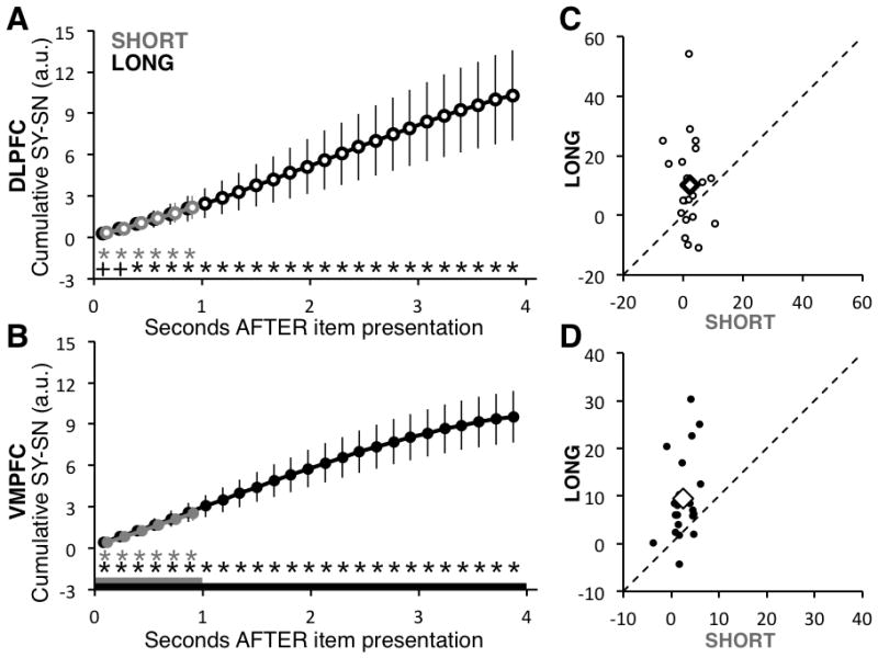
Cumulative Neural Estimate Analyses. A) Estimate of the cumulative difference in activity levels in the DLPFC ROI between trials with SY and SN responses, for each time bin and condition. The cumulative level of activity for any time bin t, subject, and condition was computed by adding the instantaneous activity levels depicted in Figure 3, from bin 0 to bin t. Gray and black bars at the bottom of the figure indicate the length of time the foods were initially shown in each condition. Gray or black asterisks indicate that the difference was significantly different than zero at p < 0.05 (pluses indicate marginally different at p < .1), based on a paired t-test computed across subjects. Note that the two curves lie almost on top of each other. B) Analogous estimates for the VMPFC ROI. Error bars are standard error of the mean calculated across participants. C) Individual estimates of the cumulative difference in DLPFC activity between trials with SY and SN responses, measured at the end of the initial non-response viewing period for each condition. Each circle denotes one subject. Black diamonds are the group mean. The dashed line indicates the line of identity. D) Analogous plot for the VMPFC ROI. A paired t-test across subjects indicates that in both cases the cumulative value signal at the end of initial item presentation was greater in the Long condition (DLPFC: p=0.04; VMPFC: p = 0.0009, N=21

Taken together, this set of results indicates the following robust properties of the DV signals in VMPFC and DLPFC. First, the DV signals were indistinguishable across conditions for the first second of computation, when the stimulus is present in both cases. Second, but they began to differ after that: the signal ramped down in the Short condition, but remained above zero for significantly longer in the long condition.

Question 2: Does extra decision time result in more accurate choices?

The computational models of choice that state that decision values must be computed and compared to make a choice suggest that the additional computation time we observed in VMPFC and DLPFC should result in more accurate choices. To determine whether this was the case, we tested for differences either in average DVs, or in the relationship between DVs and the temporally unconstrained Liking ratings (mean =0.12, and standard error of 0.08) made during Session 1. Differences in the averages, or lower explained variance in the Short versus Long conditions would indicate reduced consistency or accuracy in choices. However, we observed no evidence of changes in either measure. The mean decision values and the variance explained by Liking ratings did not differ across conditions (mean DV Short = −0.04 (0.06); mean DV Long = −0.03 (0.06); R²_Short = 0.57, R²_Long = 0.56; see Table 1). To ensure that lack of differences did not result from extra time taken by participants during the response period, we also examined reaction times. If decisions are not computed fully within 1 second, participants may use more of the response period to achieve greater accuracy. However, participants were slightly faster in the Short condition than the Long condition (average participant median reaction time (with standard errors) in Short = 345ms (12ms), in Long = 376ms (8ms); t(21) = 3.56, p = 0.002). Explanations for this small but counterintuitive difference could be the release of response inhibition in the Long condition or the greater predictability of response onset in the Short condition. Future research might seek to examine the source of this discrepancy and its consequences for the control of valuation. Regardless, these results suggest that choice accuracy was identical in the Short and Long conditions, and at ceiling¹. Despite evidence of neural differences, a computation time of one second was enough to saturate the value estimates driving behavior.

Table 1.

Mixed effect estimates for a linear regression of choices on liking ratings. For each individual and condition, the decisions made in the scanner (represented by their DVs; see Methods) were regressed against the liking ratings provided in the first experimental session. The table reports the mean estimated coefficients of the regression, as well as p-values for two-tailed groupwise one-sample t-tests against the null hypothesis that the mean estimated coefficient is zero (N=22).

	Estimated Constant Coefficient	Estimated Liking Rating Coefficient	R2
Short	−0.111 (p = 0.048)	0.481 (p = 1.6×10−15)	0.57
Long	−0.107 (p = 0.046)	0.494 (p = 5.4×10−15)	0.56
Short vs. Long two-tailed paired sample t-test	p = 0.81	p = 0.36	p = 0.80

Question 3: Do decision value signals evolve differently over time in VMPFC vs. DLPFC?

Although we observed some differences in the temporal course of DV signals in both VMPFC and DLPFC, it is also possible that there are differences between these two regions specifically in their evolution over time. This hypothesis was motivated by the informal observation that presentation times of less than 2s were sufficient to reliably engage VMPFC, but such short times led to inconsistent findings of DLPFC (Kim et al., 2008; Litt et al., 2010; Harris et al., 2011), compared to a presentation time of 4s which tended to engage both (McClure et al., 2004; Plassmann et al., 2007; Hare et al., 2008; Hare et al., 2009).

We tested the hypothesis that these regions display differences in the timing of their value computation signals (which could explain these observations) against the null hypothesis that they proceed identically and in parallel. To do so, we performed three closely related analyses: 1) identification of the peak timepoint of individuals’ SY-SN curves in each region of interest and condition; 2) computing the best fit shift for each region of the Short SY-SN curve to match the Long curve (intuitively, the point at which the two curves were the most similar); and 3) calculating the correlation, across participants, of the total accumulated decision value signal in the DLPFC and VMPFC.

The identification of peaks in the SY-SN score serve as a crude measure of the relative timing of a response. This analysis indicated no significant difference in the timing of the peaks in the Short condition (DLPFC peak = 9.8, VMPFC peak = 8.8). However, in the Long condition, the DLPFC (peak = 21.7) peaked significantly later than the VMPFC (peak = 13.4; t(20) = 2.7, p = 0.01).

To identify the shift, we minimized the sum of squared differences between the overlapping points of the Short and Long curves for each region. This yielded a shift of anywhere from zero (no shift) to 19 timepoints (3 seconds), which averaged 11.8 timepoints (1.87s) in the DLPFC, and 8.5 timepoints (1.34s) in the VMPFC. This corroborates the peak analysis, suggesting that in the Long condition, the DLPFC response was shifted later compared to VMPFC, relative to the respective original responses in the 1s condition. However, estimates of this shift were highly non-normal, bounded, and quantized, violating common fundamental assumptions of parametric tests, for which reason we limit these results to descriptive statistics.

In concert, these findings suggest subtle but significant differences in the timing of computations performed in VMPFC and DLPFC. Given this, we turned next to an investigation of differences in the content of those value signals.

Question 4: Are there differences in the information that is integrated to compute decision value signals in VMPFC and DLPFC?

Computation models posit that decision values are the result of accumulation and integration of multiple sources of information (e.g. different stimulus attributes) (Ratcliff and McKoon, 2008). Recent work suggests that value computations in VMPFC may be biased toward low-level, primary attributes of a stimulus, such as Tastiness, and that DLPFC may be required to incorporate more abstract attributes, such as Healthiness, into decisions (McClure et al., 2004; Hare et al., 2009). A natural hypothesis based on the above observations is that the differences we observed in timing may result from difference in content.

Before examining neural differences, we asked whether computation time affects the determinants of value signals driving decisions as observed behaviorally. We regressed each participant’s choices (DVs; see Methods) on their ratings of Tastiness & Healthiness of those same items, separately for the Short condition and the Long condition. If these attributes differentially predict choice as a function of time, we should see differences in the parameters across the two conditions. However, we observed little evidence of such changes. Across participants, mean (and standard error) for ratings of the food items were 0.24 (0.08) for Taste and −0.44 (0.06) for Health. In both conditions, Tastiness was the primary driver of choice (□_short = 0.474, □_long = 0.491, both ps < .01), while Healthiness played a much smaller role (□_short = 0.033, □_long = 0.056). There were no significant differences between the Short and Long conditions for any of the parameters of interest (Table 2), although Healthiness did play a marginally significant role in choices made in the Long condition (p = 0.063) but not in the Short condition (p = 0.18). Individual-level parameter significance tests also revealed no consistent patterns across conditions (not shown). In summary, there was no strong behavioral evidence that different attributes of the stimuli were driving decision values in the Short versus Long conditions.

Table 2.

Mixed effect estimates for a linear regression of choices on health and taste ratings. For each individual and condition, the decisions made in the scanner (represented by DVs; see Methods) were regressed against the Taste and Health ratings provided in the first experimental session. The table reports the mean estimated coefficients of the regression, as well as p-values for two-tailed groupwise one-sample t-tests against the null hypothesis that the mean estimated coefficient is zero (N=22).

	Estimated Constant Coefficient	Estimated Health Rating Coefficient	Estimated Taste Rating Coefficient	R2
Short	−0.158** (p = 0.0016)	0.033 (p = 0.18)	0.474 (p = 2.7×10−12)	0.54
Long	−0.155** (p = 0.0012)	0.056 (p = 0.063)	0.491 (p = 6.8×10−12)	0.56
Short vs. Long two-tailed paired sample t-test	p = 0.86	p = 0.11	p = 0.23	p = 0.42

Although we did not observe differences in the behavioral weighting of these two properties, it is still possible that different regions may differentially represent these components of value, or that such a representation interacts with the available decision time. We thus tested for neural differences in the representation of Tastiness and Healthiness in VMPFC and DLPFC by condition. To do this, we ran a second GLM regressing Tastiness and Healthiness against the BOLD response separately in the Short and Long conditions (see Methods, GLM 2). We then extracted parameter estimates for the VMPFC and DLPFC for each attribute and condition and subjected them to a 2 (Region: DLPFC & VMPFC) x 2 (Attribute: Health & Taste) x 2 (Condition: Short & Long) repeated-measures ANOVA. This analysis indicated a strong main effect of Attribute (F(1,21) = 22.4, p = 0.0001; Taste > Health), a weak main effect of Condition (F(1,21) = 3.5, p = 0.08; Short > Long), and a weak Condition x Attribute interaction (F(1,21) = 4.1, p = 0.06), driven by the decrease in responses to Taste in the Long relative to the Short condition in both regions (DLPFC t(21) = 2.1, p=0.05; VMPFC t(21) = 2.2, p = 0.04), with no similar decrease in responses to Health (all ps > 0.35) (Figure 5). Note that conclusions based on these differences are subject to the caveat that the canonical hemodynamic response, as implemented in the GLM, fits the brain activity equally well in both conditions.

Figure 5.

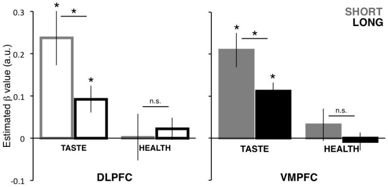
ROI analysis of BOLD responses to health and taste ratings. Average estimated beta values for each type of rating, ROI, and condition (see GLM 2). Asterisks indicate a significant difference at p < 0.05 (one-sample or paired two-tailed t-tests, as applicable). In all ROIs and conditions, Taste betas were significantly greater than Health betas (p < 0.05).

Taken together, these results suggest that there are few if any behavioral or neural differences in the attributes driving the computation of decision value.

The combination of differences in timing but not content in VMPFC and DLPFC value signals could result from a sharing of information between the two. This suggests two complementary hypotheses: 1) value signals in the two regions should be correlated, and 2) greater computation times should allow for greater convergence in their signals, leading to stronger correlations in the Long vs. Short condition. To test these hypotheses, we calculated the correlation between the total accumulated DV signal in these regions across participants. In both Short and Long conditions, these measures were highly correlated (Short: r(19) = 0.53, p = 0.01; Long: r(19) = 0.78, p = 0.00004). Moreover, the correlation in the long condition was marginally greater (one-tailed Fisher’s r-to-z, z = 1.37, p = 0.09) (Figure 6). These results provide modest support for the sharing of value-related information between these regions.

Figure 6.

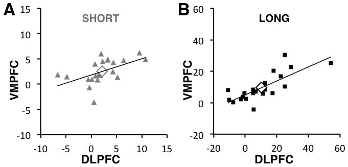
Correlations of Cumulative Neural Estimate Analyses Across Regions. A) For Short trials only: estimates of the cumulative difference in activity between trials with SY and SN responses, measured at the end of the initial 1s viewing period, in the DLPFC and VMPFC ROIs. Each circle denotes one subject. Black diamonds are the group mean. The line indicates the best fit regression. B) Analogous plot for the Long condition. Plot shows that in both conditions there is a positive correlation between the estimate in both ROIs (Short: r(19) = 0.53, p = 0.01; Long: r(19) = 0.78, p = 0.00004; Pearson’s correlation; N=21).

DISCUSSION

In this study, we address four questions related to whether and how available computation time affects neural decision value signals and behavioral responses. We found that while the available computation time did not change choices or the attributes driving them, decision value signals in the DLPFC and VMPFC showed marked intra-and interregional differences, providing novel constraints on our understanding of decision values.

Previous studies involving different species and techniques have found that activity in VMPFC and DLPFC reflects the computation of DV signals (Rangel and Hare, 2010; Wallis and Kennerley, 2010; Padoa-Schioppa, 2011), which are then compared to make a choice (Basten et al., 2010; Milosavljevic et al., 2010; Hare et al., 2011b). Activity in the same regions also correlated with DVs in the current study, in both the Short and the Long conditions. This provides additional support in favor of the hypothesis that these two areas are central to the computation of DVs, and hence choices. But the main goal of the study was to extend this literature, by characterizing several unknown properties of the DV signals encoded in these two regions, including their relationship to choices, and signals in these areas differ and interact. Our findings support the following conclusions.

Finding 1

The temporal profile of DV signals depends on the available decision time. In particular, during the first second of the trial, the signals were indistinguishable across the Short and Long conditions, but began to diverge thereafter. This suggests that these value computations were sensitive to the presence of the stimulus and/or the onset of the response window. In particular, in the Short condition, DV signals in both regions began ramping down after the viewing window ended and a response was required, but remained high in the Long condition through its entire four second length, only ramping down at the end.

This finding provides useful insights about the nature of the DV computations. First, it shows that in our task the computation of DVs expands to fit the available computation time (and in fact may extend beyond this point in the Short condition). This stands in contrast to neurophysiological studies which suggest that evidence accumulation in parietal neurons during perceptual tasks continues only until a decision threshold is crossed and no further, even if there is more computation time available (Kiani et al., 2008; Kiani and Shadlen, 2009). Since there are many differences between the two tasks, an important question for future work will be to characterize what determines the duration of basic perceptual and valuation computations, across a wide variety of tasks. Second, although the start and end of DV computation aligns well with the presence of the stimulus, suggesting that valuation is strictly stimulus-locked. However, we think our data suggest a more complex relationship. Specifically, there is evidence that these computations may not be strictly stimulus locked as DV computation in the Short condition continues after, and in the Long condition stops before the response has been entered and the stimulus is removed from the screen.

It is important to acknowledge that there may be alternative explanations for these response profiles. For example, neural adaptation could account for some of the differences across the Short and Long conditions; alternatively, the observed value signals may represented the maintenance of a stored value signal and not its ongoing computation. The overwhelming evidence that these regions engage in active and consequential DV computation argues against these interpretations, but future work will be necessary to fully address these alternatives. For example to test whether adaptation explains the patterns of the observed neural estimates, future studies could vary the length of the viewing window, repeat items a variable number of times, prime item presentations with other objects, or vary the stimuli to be simpler or more complex. Observing how computation might change in these cases could shed light on these possible explanations.

Finding 2

The Long condition resulted in greater cumulative DV signals in both ROIs. This larger cumulative signal could be interpreted to indicate a stronger representation of value, which could have implications for the quality and reliability of downstream processes. Although the increase in available decision time did not lead to improvements in choice quality in this study, our results are consistent with previous studies of speed-accuracy trade-offs in valuation (Ratcliff and McKoon, 2008; Milosavljevic et al., 2010; Milosavljevic et al., 2011).

This finding also provides additional insights into the nature of the valuation process. First, it shows that the DVs are not computed using a computationally efficient process. Specifically, we found that they continued after the response in the Short condition, and that choices were no different across conditions despite an almost five-fold difference in the total amount of computation. This seems highly inefficient since computation is metabolically costly (Kandel et al., 2000), and in the above cases either cannot or did not affect choices. It is possible the additional computation would have effects on other aspects of behavior we did not observe (e.g. learning, changes over time, etc.), but this remains a question for future research.

This inefficiency also suggests that DV signals need only be of sufficient quality for consistent, accurate choice (for example, to average out the noise). This is consistent with a growing number of studies finding that values are compared to make a choice using algorithms that resemble a Drift-Diffusion Model (Gold and Shadlen, 2002; Bogacz et al., 2006; Basten et al., 2010; Krajbich et al., 2010; Milosavljevic et al., 2010; Hare et al., 2011b). In these models the comparison process terminates when the cumulative DV signal crosses a pre-specified barrier. As a consequence, further improvements in the signal beyond that point in time do not affect choices. Participants’ choices in our study were highly accurate in both conditions, which suggests that even in the Short condition, the amount of signal computed was sufficient to cross the associated barriers. This could explain why the additional calculation of the DVs in the Long condition did not improve choice quality.

How can we reconcile our findings of consistently accurate choices with evidence that neural estimates of value signals extend beyond the effective or necessary amount of time? Recent research suggests that value signals may be used after choice for other reasons, including online response adjustment or inter-trial learning, as proposed elsewhere (Resulaj et al., 2009; Ding and Gold, 2011).

Finding 3

In the Long condition, DV signals of equivalent magnitude appeared later in DLPFC than in VMPFC. A similar difference could not be found for the Short condition, though a careful look at Figure 3 suggests that the null results for the Short condition might be the product of limited statistical power. Nevertheless, this finding is consistent with previous studies of the DV signals in monkeys (Wallis and Miller, 2003), which also found that the DLPFC signal lagged the one in VMPFC. The authors’ interpretation of the delay was that the VMPFC value signals were subsequently passed to DLPFC to influence the selection of motor responses. This interpretation is inconsistent with recent fMRI studies of the network involved in making choices (Basten et al., 2010; Hare et al., 2011b), which find that the DLPFC plays a role in controlling the comparison process, but that its activity does not reflect the computation of DVs. Regardless of the precise computational relationship between the two regions, we demonstrate that they do not have the same temporal profile, and specifically that computation in the DLPFC is shifted later relative to the VMPFC. Such a temporal difference could arise, for example, if the two areas used different inputs to compute the DVs, which were themselves computed with different latencies, or if value information was shared between these regions, as mentioned above.

Finding 4

VMPFC and DLPFC, contrary to hypotheses that these regions would represent different attributes, were equally sensitive to Tastiness and Healthiness of foods, two attributes that can be used to compute DVs (Basten et al., 2010; Rangel and Hare, 2010). Others have argued that VMPFC signals may reflect the integration of ‘basic attributes’ (e.g., taste), whereas DLPFC may reflect the integration of ‘abstract attributes’ (e.g., health) (McClure et al., 2004; Hare et al., 2011a). However, an important caveat to conclusions in the current study was the weak behavioral relationship we observed between Healthiness and DVs. It is possible that if participants had been more motivated to consider Healthiness in their choices (e.g. were dieting), we would have observed differences within and between the DLPFC and VMPFC signals. Regardless, our findings are not fully consistent with this view, since the relative weight of Tastiness, which was tightly linked to decision value, were represented similarly in both areas. The results also show that the ability of DLPFC to consider more abstract attributes, such as health, does not necessarily increase with additional computational time. Future research will be needed to examine how Healthiness, and other attributes not considered here, may play a role in the computation of decision value, and interact with longer amounts of decision time.

By controlling the amount of time in which a very simple choice must be reached, this study provides a lower bound on the consequences of altering the temporal constraints of valuation. Value circuitry shifts computation to accommodate the time given. That it did so was not a foregone conclusion. This suggests both a high degree of neural flexibility at the cost of efficiency, but limited exploitation of the available time. Value computation may be basic, or even primitive, but it is also a remarkably flexible process, sensitive to both external constraints and internal control.

ABBREVIATIONS

fMRI

functional magnetic resonance imaging

GLM

general linear model

FIR

finite impulse response

DLPFC

dorsolateral prefrontal cortex

VMPFC

ventromedial prefrontal cortex

ITI

inter-trial interval

BOLD

blood-oxygenation-level dependent [signal]

HRF

hemodynamic response function

DV

decision value

References

- Basten U, Biele G, Heekeren HR, Fiebach CJ. How the brain integrates costs and benefits during decision making. PNAS. 2010;107(50):21767–21772. doi: 10.1073/pnas.0908104107. [DOI] [PMC free article] [PubMed] [Google Scholar]
- Baumgartner T, Knoch D, Hotz P, Eisenegger C, Fehr E. Dorsolateral and ventromedial prefrontal cortex orchestrate normative choice. Nat Neurosci. 2011;14(11):1468–1474. doi: 10.1038/nn.2933. [DOI] [PubMed] [Google Scholar]
- Bogacz R, Brown E, Moehlis J, Holmes P, Cohen JD. The physics of optimal decision making: a formal analysis of models of performance in two-alternative forced-choice tasks. Psychol Rev. 2006;113(4):700–765. doi: 10.1037/0033-295X.113.4.700. [DOI] [PubMed] [Google Scholar]
- Deichmann R, Gottfried JA, Hutton C, Turner R. Optimized EPI for fMRI studies of the orbitofrontal cortex. NeuroImage. 2003;19:430–431. doi: 10.1016/s1053-8119(03)00073-9. [DOI] [PubMed] [Google Scholar]
- Ding L, Gold JI. Neural Correlates of Perceptual Decision Making before, during, and after Decision Commitment in Monkey Frontal Eye Field. Cereb Cortex. 2011 doi: 10.1093/cercor/bhr178. [DOI] [PMC free article] [PubMed] [Google Scholar]
- Figner B, Knoch D, Johnson EJ, Krosch AR, Lisanby SH, Fehr E, et al. Lateral prefrontal cortex and self-control in intertemporal choice. Nat Neurosci. 2010;13(5):538–539. doi: 10.1038/nn.2516. [DOI] [PubMed] [Google Scholar]
- Friston KJ, Poline JB, Holmes AP, Frith CD, Frackowiak RSJ. A multivariate analysis of PET activation studies. Human Brain Mapping. 1996;4:140–151. doi: 10.1002/(SICI)1097-0193(1996)4:2<140::AID-HBM5>3.0.CO;2-3. [DOI] [PubMed] [Google Scholar]
- Gitelman DR, Penny WD, Ashburner J, Friston KJ. Modeling regional and psychophysiologic interactions in fMRI: the importance of hemodynamic deconvolution. Neuroimage. 2003;19(1):200–207. doi: 10.1016/s1053-8119(03)00058-2. [DOI] [PubMed] [Google Scholar]
- Gold JI, Shadlen MN. Banburismus and the brain: decoding the relationship between sensory stimuli, decisions, and reward. Neuron. 2002;36(2):299–308. doi: 10.1016/s0896-6273(02)00971-6. [DOI] [PubMed] [Google Scholar]
- Hare TA, Camerer CF, Rangel A. Self-Control in Decision-Making Involves Modulation of the vmPFC Valuation System. Science. 2009;324(5927):646–648. doi: 10.1126/science.1168450. [DOI] [PubMed] [Google Scholar]
- Hare TA, Malmaud J, Rangel A. Focusing attention on the health aspects of foods changes value signals in vmPFC and improves dietary choice. J Neurosci. 2011a;31(30):11077–11087. doi: 10.1523/JNEUROSCI.6383-10.2011. [DOI] [PMC free article] [PubMed] [Google Scholar]
- Hare TA, O'Doherty JP, Camerer CF, Schultz W, Rangel A. Dissociating the role of the orbitofrontal cortex and the striatum in the computation of goal values and prediction errors. J Neurosci. 2008;28(22):5623–5630. doi: 10.1523/JNEUROSCI.1309-08.2008. [DOI] [PMC free article] [PubMed] [Google Scholar]
- Hare TA, Schultz W, Camerer CF, O'Doherty JP, Rangel A. Transformation of stimulus value signals into motor commands during simple choice. PNAS. 2011b;108(44):18120–18125. doi: 10.1073/pnas.1109322108. [DOI] [PMC free article] [PubMed] [Google Scholar]
- Harris A, Adolphs R, Camerer CF, Rangel A. Dynamic construction of stimulus values in the ventromedial prefrontal cortex. PLoS ONE. 2011;6(6):e21074. doi: 10.1371/journal.pone.0021074. [DOI] [PMC free article] [PubMed] [Google Scholar]
- Kable JW, Glimcher PW. The neural correlates of subjective value during intertemporal choice. Nat Neurosci. 2007;10(12):1625–1633. doi: 10.1038/nn2007. [DOI] [PMC free article] [PubMed] [Google Scholar]
- Kandel ER, Schwartz JH, Jessell TM, editors. Principles of Neural Science. New York: McGraw-Hill; 2000. [Google Scholar]
- Kiani R, Hanks TD, Shadlen MN. Bounded integration in parietal cortex underlies decisions even when viewing duration is dictated by the environment. J Neurosci. 2008;28(12):3017–3029. doi: 10.1523/JNEUROSCI.4761-07.2008. [DOI] [PMC free article] [PubMed] [Google Scholar]
- Kiani R, Shadlen MN. Representation of confidence associated with a decision by neurons in the parietal cortex. Science. 2009;324(5928):759–764. doi: 10.1126/science.1169405. [DOI] [PMC free article] [PubMed] [Google Scholar]
- Kim S, Hwang J, Lee D. Prefrontal coding of temporally discounted values during intertemporal choice. Neuron. 2008;59(3):161–172. doi: 10.1016/j.neuron.2008.05.010. [DOI] [PMC free article] [PubMed] [Google Scholar]
- Krajbich I, Armel C, Rangel A. Visual fixations and the computation and comparison of value in simple choice. Nat Neurosci. 2010;13(10):1292–1298. doi: 10.1038/nn.2635. [DOI] [PubMed] [Google Scholar]
- Litt A, Plassmann H, Shiv B, Rangel A. Dissociating valuation and saliency signals during decision-making. Cereb Cortex. 2010;21(1):95–102. doi: 10.1093/cercor/bhq065. [DOI] [PubMed] [Google Scholar]
- Mars RB, Jbabdi S, Sallet J, O'Reilly JX, Croxson PL, Olivier E, et al. Diffusion-Weighted Imaging Tractography-Based Parcellation of the Human Parietal Cortex and Comparison with Human and Macaque Resting-State Functional Connectivity. Journal of Neuroscience. 2011a;31(11):4087–4100. doi: 10.1523/JNEUROSCI.5102-10.2011. [DOI] [PMC free article] [PubMed] [Google Scholar]
- Mars RB, Sallet J, Schüffelgen U, Jbabdi S, Toni I, Rushworth MFS. Connectivity-Based Subdivisions of the Human Right "Temporoparietal Junction Area": Evidence for Different Areas Participating in Different Cortical Networks. Cereb Cortex. 2011b:1–10. doi: 10.1093/cercor/bhr268. [DOI] [PubMed] [Google Scholar]
- McClure SM, Laibson DI, Loewenstein G, Cohen JD. Separate neural systems value immediate and delayed monetary rewards. Science. 2004;306(5695):503–507. doi: 10.1126/science.1100907. [DOI] [PubMed] [Google Scholar]
- Milosavljevic M, Koch C, Rangel A. Consumers can make decisions in as little as a third of a second. Judgment and Decision Making. 2011;6(6):520–530. [Google Scholar]
- Milosavljevic M, Malmaud J, Huth A, Koch C, Rangel A. The Drift Diffusion Model can account for the accuracy and reaction time of value-based choices under high and low time pressure. Judgment and Decision Making. 2010;5(6):437–449. [Google Scholar]
- O'Reilly JX, Beckmann CF, Tomassini V, Ramnani N, Johansen-Berg H. Distinct and Overlapping Functional Zones in the Cerebellum Defined by Resting State Functional Connectivity. Cereb Cortex. 2010;20(4):953–965. doi: 10.1093/cercor/bhp157. [DOI] [PMC free article] [PubMed] [Google Scholar]
- Padoa-Schioppa C. Neurobiology of economic choice: a good-based model. Annual Review of Neuroscience. 2011;34:333–359. doi: 10.1146/annurev-neuro-061010-113648. [DOI] [PMC free article] [PubMed] [Google Scholar]
- Plassmann H, O'Doherty JP, Rangel A. Orbitofrontal cortex encodes willingness to pay in everyday economic transactions. J Neurosci. 2007;27(37):9984–9988. doi: 10.1523/JNEUROSCI.2131-07.2007. [DOI] [PMC free article] [PubMed] [Google Scholar]
- Plassmann H, O'Doherty JP, Rangel A. Appetitive and aversive goal values are encoded in the medial orbitofrontal cortex at the time of decision making. J Neurosci. 2010;30(32):10799–10808. doi: 10.1523/JNEUROSCI.0788-10.2010. [DOI] [PMC free article] [PubMed] [Google Scholar]
- Rangel A, Hare T. Neural computations associated with goal-directed choice. Current Opinion in Neurobiology. 2010;20(2):262–270. doi: 10.1016/j.conb.2010.03.001. [DOI] [PubMed] [Google Scholar]
- Ratcliff R, McKoon G. The Diffusion Decision Model: Theory and Data for Two-Choice Decision Tasks. Neural Computation. 2008;20:873–922. doi: 10.1162/neco.2008.12-06-420. [DOI] [PMC free article] [PubMed] [Google Scholar]
- Resulaj A, Kiani R, Wolpert DM, Shadlen MN. Changes of mind in decision-making. Nature. 2009;461(7261):263–266. doi: 10.1038/nature08275. [DOI] [PMC free article] [PubMed] [Google Scholar]
- Rushworth MF, Noonan MP, Boorman ED, Walton ME, Behrens TE. Frontal cortex and reward-guided learning and decision-making. Neuron. 2011;70(6):1054–1069. doi: 10.1016/j.neuron.2011.05.014. [DOI] [PubMed] [Google Scholar]
- Wallis JD, Kennerley SW. Heterogeneous reward signals in prefrontal cortex. Current Opinion in Neurobiology. 2010;20(2):191–198. doi: 10.1016/j.conb.2010.02.009. [DOI] [PMC free article] [PubMed] [Google Scholar]
- Wallis JD, Miller EK. Neuronal activity in primate dorsolateral and orbital prefrontal cortex during performance of a reward preference task. European Journal of Neuroscience. 2003;18(7):2069–2081. doi: 10.1046/j.1460-9568.2003.02922.x. [DOI] [PubMed] [Google Scholar]
Associated Data
This section collects any data citations, data availability statements, or supplementary materials included in this article.