Spatial information analysis of chemotactic trajectories

Abstract

During bacterial chemotaxis, a cell acquires information about its environment by sampling changes in the local concentration of a chemoattractant, and then uses that information to bias its motion relative to the source of the chemoattractant. The trajectory of a chemotaxing bacteria is thus a spatial manifestation of the information gathered by the cell. Here we show that a recently developed approach for computing spatial information using Fourier coefficient probabilities, the k-space information (kSI), can be used to quantify the information in such trajectories. The kSI is shown to capture expected responses to gradients of a chemoattractant. We then extend the k-space approach by developing an experimental probability distribution (EPD) that is computed from chemotactic trajectories collected under a reference condition. The EPD accounts for connectivity and other constraints that the nature of the trajectories imposes on the k-space computation. The EPD is used to compute the spatial information from any trajectory of interest, relative to the reference condition. The EPD-based spatial information also captures the expected responses to gradients of a chemoattractant, although the results differ in significant ways from the original kSI computation. In addition, the entropy calculated from the EPD provides a useful measure of trajectory space. The methods developed are highly general, and can be applied to a wide range of other trajectory types as well as non-trajectory data.

Introduction

Bacterial chemotaxis is a simple example of an organism acquiring information from the environment and making purposeful use of that information [1]. In this system, the bacterium acts as an “observer” that gathers information, such as the local concentration of a chemoattractant, and uses the information to modify its swimming trajectory. In particular, the movement of a bacterium in a gradient of a chemoattractant is biased relative to spatial differences in concentration. Bacterial swimming is characterized by two types of behaviors, runs in which swimming is an uninterrupted forward movement and tumbles in which the bacteria stops and turns. The biased movement along a gradient is achieved by changing the balance of runs and tumbles. By increasing the frequency of tumbles under relatively unfavorable conditions and decreasing the frequency under favorable conditions, a movement toward more favorable conditions is produced. Chemotaxis in E. coli has been especially well studied, and the biochemical pathways that connect sensing of the chemoattractant to the biased motion are well understood [2, 3]. Further, the physical parameters of the E. coli swimming have been well characterized [1, 3]. Together with advances in computational capabilities, this has led to the development of several computational models that reproduce experimental measurements of bacterial swimming trajectories [3, 4].

Chemotactic trajectories, records of the path taken by a cell over some period of time, have been extensively studied. For bacterial chemotaxis, the path of motion has been shown to be well modeled as a biased diffusion [5], although one recent study suggests that, at least in some instances, chemotaxis is better characterized as a fractional Brownian motion [6]. Information theoretic approaches have been used to quantify trajectories of chemotaxing Dictyostelium cells [7, 8]. In that case, the trajectories are typically reduced to a set of angles that reflect the direction a cell is moving at different points in time, from which a measure of information is computed. The relationship of the angle distributions to the orientation of a gradient can then be quantified to provide some insight into how spatial information in the gradient is converted to information in the movement of the cells. However, this angle-based approach to quantifying the information in a trajectory has the potential to produce some counter-intuitive results. As an extreme example, a cell performing a random walk would have the same angle entropy as one swimming in a perfect circle. Here we present a new approach for quantifying chemotactic trajectories that overcomes this limitation and has a number of useful properties, and then test it on simulated trajectories from chemotaxing bacteria.

We define information as the reduction of uncertainty. The Shannon formalism for information theory considers information transfer between a sender and a receiver. From the perspective of the receiver, there is some uncertainty before a message (information) is received and some smaller uncertainty after it is received [9]. For a cell moving in a uniform environment, there is at any given time a high degree uncertainty of where it is and in what direction it is moving, relative to some point of reference. However, if we introduce a chemoattractant, the movement of the cell becomes biased, and there is less uncertainty about the cell’s movements. It will be more likely be close to the source of the chemoattractant than far away, and more likely to be swimming toward the chemoattractant than in other directions. This reduction of uncertainty is a reflection of the information that the cell gathered from the chemoattractant. We can also look at trajectories in terms of how frequently they occur. For example, for a bacterium that starts swimming in the center of a shallow Petri dish, in the absence of a chemoattractant, there is some universe of possible trajectories it might take over the next 5 min. Out of all of these trajectories, the bacterium will usually swim and tumble in a path that is not biased in any particular direction. Recalling in mind the limitations discussed above, if one measures the angle at which it is swimming at random points in time—these angles will be close to uniformly distributed between 0° and 360°. The trajectories that meet this criterion are for our purposes thereby equivalent, and form a very large subset of all possible trajectories. Any one of these trajectories would be considered common, and therefore have low information. In contrast, on a very (very) rare occasion, a bacterium might start at the center of a test tube and swim straight toward the edge of the dish, without turning. There are a relatively small number of unique ways to form this path, and this constitutes a small subset of all possible trajectories. Any one of these trajectories would be considered uncommon, and would therefore have high information. Thus common trajectories reflect a high degree of uncertainty, and rare trajectories reflect less uncertainty.

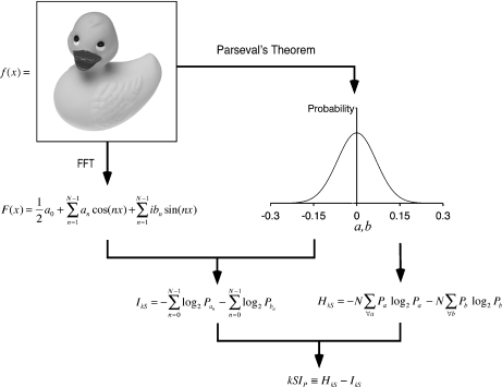
We have recently developed a new formalism to compute the information in an arbitrary data object, in which the data object is recast via a Fourier transform and the likelihoods of the Fourier coefficients from this transform are used to compute a measure of how likely or unlikely it is that the object would have occurred randomly (Fig. 1) [10]. The k-space information (kSI) metric is a general way to compute a value for the information in a data object produced under any particular constraints of interest, and the kSI is small for a common object and large for a rare object. In the case where the data object is a spatially defined collection of values, such as a bacterial trajectory, the kSI is a measure of the spatial information. The original implementation of the kSI metric was based on using Parseval’s theorem to obtain a probability distribution of the Fourier coefficients in some data object (e.g., an image). This is the least constrained approach, and it depends on only the dimensions of the data object and the composition of elements in the object. Thus, for an image, the Parseval’s distribution depends on the size and histogram. We use an image format in which the histogram is identical for all images of a certain size, and in this case the Parseval’s distribution accounts for all possible images of that size. We here refer to this Parseval’s-based probability distribution as the PPD.

Fig. 1.

Schematic illustrating how information is computed in k-space using the Parseval’s-based probability distribution (adapted from [11]). Starting with a data object f(x) with N elements, here using an image of a duck as an example, a probability distribution is computed using Parseval’s theorem (the PPD). The PPD is Gaussian, and gives the probability distribution of the Fourier coefficients for all possible images of the same size and histogram as f(x). An entropy (H_kS) is then computed from this distribution. The data object is then Fourier transformed to F(x), and an information (I_kS) based on the Fourier coefficients in F(x) is computed using the PPD. The kSI_P is then defined as the difference between the I_kS and the H_kS

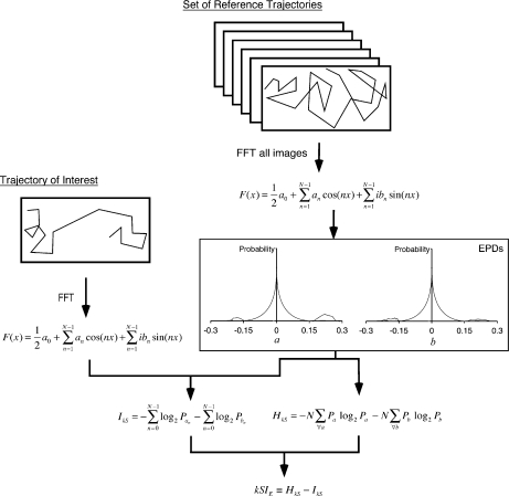
Here we begin by applying the kSI formalism to analyzing the information in simulated chemotactic trajectories, and show that the k-space information can be used to quantify information that is reflected in the trajectories. We then proceed to extend the k-space formalism to account for physical constraints that are imposed by the system. For bacterial trajectories, there are a number of constraints that will be reflected in the probability distributions. For example, the points in a bacterial trajectory must be connected; there are no trajectories in which a bacterium hops between disconnected points in a field. These constraints are not accounted for in the PPD, which could influence the use of the kSI in ways that are not understood. We address this limitation by developing an experimental probability distribution (EPD) that is system-specific. The idea is to collect Fourier coefficients from a large number of chemotactic trajectories obtained under a reference condition, and use these coefficients to estimate a probability distribution for the Fourier coefficients of all possible trajectories subject to the constraints of the reference condition. The EPD is then used to compute an information value essentially as described above. This information is a measure of how rare or how common a particular trajectory is under some set of constraints, relative to trajectories in the reference state. To distinguish kSI values computed with the different distributions, we use the subscripts E for experimental and P for Parseval’s.

Chemotaxis was simulated using a program developed by Bray and coworkers [3, 6], where the underlying biochemistry is based on the well-established BCT program [3]. Specifically, we use the version of the program described Zonia and Bray [6]. The Zonia and Bray Program (ZBP) simulates a bacterium swimming in a two-dimensional arena, where the concentration and distribution of a chemoattractant can be controlled. Here aspartic acid was used as the chemoattractant and the gradients were exponential. The bacteria were wild-type, although the program allows extensive control over the genetic properties and physical behavior of the bacterium. The output from the program is a real-time graphical display of the current position of a bacterium as a function of time and a step-wise list of xy coordinates at 0.1 μm increments for the trajectory. For our purposes, trajectories are then converted in graphical representations of the entire path followed by a bacterium, trajectory plots, which are used for the information analysis. The behavior of bacteria in this model has been shown to agree well with experiments [3, 6].

Methods

Simulation of bacterial chemotaxis

We use the ZBP program developed by Bray and coworkers to simulate chemotaxis [6]. The C+ + source code for the program was generously provided by Dr. Dennis Bray. Some modifications to the code as received where made. To shorten the simulation duration, the time step for the graphical display was reduced from 25 ms to 1 ms. Several tests were performed to show that the shorter time step only changed the speed of the real-time display, but otherwise produced trajectories identical to the longer time step. Further, the contrail size was reduced to 10. An infectivity value of 35 was used, except where indicated. This effectively set the chemoattractant concentration range over which the bacterium was responsive to 1×10^− 9 M to 5×10^− 7 M. The original program used a tumble angle of +/−72° centered at zero. This was modified to an angle centered at +/−68° with a standard deviation of 36°, based on the experimental values [11, 12]. The angle resolution was also reduced from 10° to 1°. Simulations were run on Intel-based Macintosh computers running OSX version 10.5 or higher.

Producing trajectory plots

Trajectories were converted to three-dimensional binary surfaces for the information computations. The ZBP program outputs trajectories in steps of 0.1 μm. However, to simplify the computation, we plotted this data into a 400 × 800 μm arena divided into 1 x 1 μm pixels in the plane. The arena also has an 8-bit third dimension (z) to account for trajectories crossing the same pixel multiple times. The voxels within the arena are binary, and thus have value of 0 or 1. For the k_Max arena, the z = 0 voxels values are initially set to 1 and all other voxels are set to 0. As a bacterium swims through the arena it visits different xy positions, and each time it crosses the boundary between two xy pixels, the z value for the xy position being entered is incremented. Thus, the more times a bacterium crosses the same xy position, the larger the z value for that position. This representation has several important features. First, it accounts for bacteria revisiting the same areas of the arena many times. Second, the image histograms of all possible trajectories (for a given arena size) are identical. There are 400 × 800 voxels with the value 1, and 400 × 800 × 255 voxels with the value 0. This holds for all trajectories, until any given point within the arena has been visited more than 255 times. In a 100,000 step simulation, it was very rare for a position to be visited more than 20 times, and thus the z limit of the arena was not an issue. Trajectory plots in the k_Min arena were created in the same way, except that the empty arena was first populated (value set to 1) at random z values (one z value for each xy position). The first time a position was visited in a k_Min arena, the z = 1 voxel was set to 1, and then incremented as above.

Computing the spatial information

The kSI_P is computed from a trajectory plot. In this approach, we use Parseval’s theorem to compute a probability distribution for all possible images of a given size (when using the binary surface representation) [11]. Parseval’s theorem equates the sum of the square of a function with the sum of the square of the Fourier transform for the function:

1

Here, f is a function of x and y, and F is the corresponding Fourier transform with the indices m and n. C is a constant, N is the number of elements in f, and σ is the standard deviation of the distribution of the Fourier coefficients. Treating the coefficients as independent identically distributed random variables [13] and invoking the central limit theorem, we obtain a Gaussian probability distribution. The information for an image is then computed using the PPD as outlined in Fig. 1.

To compute the kSI_E for a trajectory plot, we typically begin with 1,216 trajectories computed under a reference condition. These trajectories are used to build a Fourier coefficient probability distribution from which a kSI_E is computed. We use a uniform arena of 10^− 9 M aspartic acid as the point of reference, and trajectory lengths of 100,000 steps (10,000 μm) (unless otherwise specified). The bacteria are wild-type. The EPDs are constructed by first converting the reference trajectories to trajectory plots. The number of trajectories was selected to balance computational time and precision, which is addressed in more detail below. Fourier transforms of these trajectory plots produce ~10¹¹ Fourier coefficients. The real and imaginary parts of these coefficients are each binned and normalized to form an EPD for each. The kSI_E is then computed in a similar manner to the kSI_P, but using the two EPDs (Fig. 2).

Fig. 2.

Schematic illustrating the new approach described here for computing the k-space information for chemotactic trajectories using experimental probability distributions. In this approach, the probability distribution is established using the Fourier coefficients from a number of chemotactic trajectories collected under some reference condition. These distributions (the EPDs), for the real and imaginary parts of the coefficients, are used in place of the PPD to compute a kSI_E. Note that the EPDs shown are schematic, but they do not have a simple analytical shape

Results and discussion

Rendering the trajectory plot: k_Max versus k_Min arenas

Conversion of the trajectory coordinates to a trajectory plot requires making some choices about the form of the plot. The most direct approach is to start with an empty image of the arena, and then increment the z-value at each xy position each time the bacterium visits that coordinate (Fig. 3). This produces a familiar representation where the path of the bacterium is seen against a uniform (typically white) background. Because the kSI_P for the empty arena is effectively the maximum possible, these are called k_Max arenas. Alternatively, an arena can first be populated by a random value at each xy position. The kSI_P for an arena of this type is in practice almost always ∼0, and thus these are called k_Min arenas. The trajectory is then introduced into either arena by setting the z value of an xy coordinate to 1 the first time it is visited, and subsequently incrementing each time the bacterium crosses that position. While these two arena types start from opposite limits, they converge as the trajectories become long enough that each point in the arena has been visited at least once. While these two types of arenas produce similar results, we have elected to use the k_Max arenas (unless otherwise specified).

Fig. 3.

Trajectory plots for a 10,000-step-long simulation of a wild-type bacterium chemotaxing in an exponential gradient of aspartic acid from 1×10^− 9 M at the edges to 5×10^− 7 M at the center (red dashed line). The boundaries are periodic such that a bacterium that exits on the top side of the arena re-enters on the bottom side, or one that exits on the left re-enters on the right. The simulation was equilibrated for 50,000 steps prior to collecting the coordinates used, as described below. The same trajectory is shown plotted in a k_Max arena (left) and a k_Min arena (right). The brightness and contrast in the images was adjusted to clearly show the paths, thus the images do not provide an accurate representation of the z axis of the images

Equilibration length

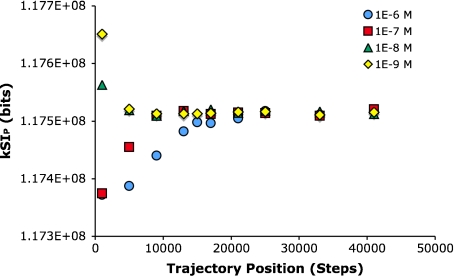
The ZBP program is a complex simulation of chemotaxis that includes a number proteins and biochemical reactions, for which there are concentrations, kinetic parameters, and other variables. The simulations do not start with these parameters optimized for any given set of conditions, and there is thus an equilibration time. In most cases, it is desirable to remove the unequilibrated parts of the trajectories to remove influences of initial parameters. To characterize the equilibration dynamics, changes in the spatial information of short trajectory segments obtained from the first 50,000 steps of a simulation were examined. For these tests, 50,000 step trajectories were computed for uniform aspartic acid concentrations of 1×10^− 6 M, 1×10^− 7 M, 1×10^− 8 M and 1×10^− 9 M (with a random starting point and random starting angle). The trajectories were then subdivided into a set of 2,000 step segments, and the kSI_P for the trajectory plot of each of these segments was computed (Fig. 4). The PPD is sufficient here because we are simply seeking to determine when the equilibration is achieved, and using the EPD is unduly laborious. The results from this analysis show that bacteria take the longest to equilibrate in the highest concentrations of aspartate, and the shortest time at the two lowest concentrations examined. For the 1×10^− 3 M case, the equilibration is complete for the trajectory at ∼24,000 steps. For the lower concentrations, the equilibration appears to be complete by ∼10,000 steps. Thus, to ensure that the starting parameters do not influence the trajectories, the first 50,000 steps were discarded. So to produce the 100,000-step trajectories used in the present work, a simulation was run to 150,000 steps and the trajectory plot was generated from steps 50,001 to 100,000.

Fig. 4.

Equilibration dynamics of simulations of a wild-type bacterium in uniform aspartic acid concentrations. The spatial information in trajectory plots from 2,000 step segments along a 50,000-step trajectory are computed and plotted. Each data point is an average of 100 trajectories

Experimental probability distributions

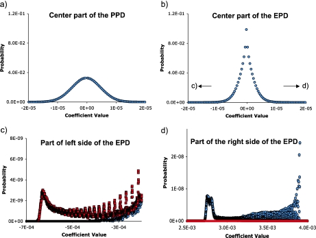
To account for deviations from the PPD that arise from constraints in a system, an experimental probability distribution was constructed by producing a large number of randomly generated bacterial trajectories under conditions that serve as a point of reference. The EPD has a form quite different from the PPD (Fig. 5). In broad strokes, very small and very large coefficient values are more common in the EPD. The central part of the EPD distributions of the real and imaginary coefficients are essentially identical, but further toward the edges of the distribution there are significant differences (Fig. 5c, d). The EPD coefficients at the largest values are >700 SD from the mean of PPD, and arise from the white background in the k_Max arena. This is because while coefficients that derive from white sections of the arena are common in the EPD, they are exceptionally rare in the PPD.

Fig. 5.

Example of an EPD for bacterial chemotaxis and comparison with the PPD. The Fourier coefficients from 1,216 trajectory plots were histogrammed and normalized. The real and imaginary parts are treated independently. The probability space is quite large, and 20,000 bins are used in order to provide sufficient resolution. Thus, only small sections of the distributions are shown. The PPD is computed as described earlier [11]. a The central part of the PPD for an 800 × 400 pixel 8-bit image. This distribution is Gaussian with a standard deviation of 4.86×10^− 6. The distributions of the real and imaginary parts of the coefficient are indistinguishable, and only the real coefficients are shown (blue circles). b The central part of the EPD for 100,000 step trajectories of a wild-type bacterium in a 800 × 400 μm arena with a uniform concentration of 1 × 10^− 9 M aspartic acid. Here again the distributions of the real and imaginary parts of the coefficient are indistinguishable. c High-resolution view of the left side of the EPD, illustrating how non-uniform the distribution is, and showing differences between the distributions of the real (blue circles) and imaginary (red squares) parts. d High-resolution view of the right side of the EPD, near the limit of the distribution. Notably, these coefficients are ∼700 standard deviations from the mean. Symbols are as in c

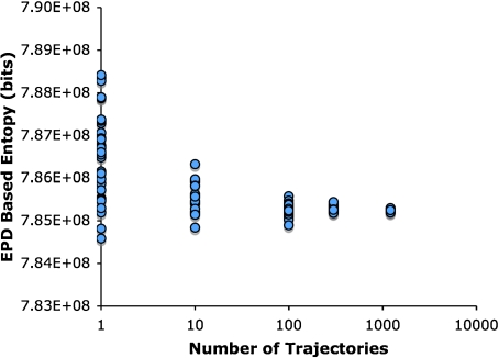
The number of trajectories used to compute the EPD was selected to balance adequate sampling with computational resources. To establish adequate sampling, the entropy from the probability distribution was computed as a function of the number of trajectories in the EPD (Fig. 6). Somewhat surprisingly, even for individual trajectories, the coefficient of variance for the trajectory plot entropy is only 0.14%. At 1,216 trajectories (∼1×10¹¹ coefficients) the entropy of variance falls to 0.004% (∼35 kbits). With the resources at our disposal, an EPD based on 1,216 trajectories takes about 2 CPU days to compute, which includes computing the trajectories, converting the trajectories into trajectory plots, and computing the EPD. While this process could likely be significantly shortened by optimizing the programs used, it at present represents an acceptable balance of precision and time for our purposes.

Fig. 6.

Convergence of experimental probability distributions. The entropy is computed from the probability distributions by summing -PLog₂P for each bin in the distribution, and averaging this value for the number of trajectories indicated. The downward trend in the mean arises from the padding of zero values with 1, the effect of which makes a significant contribution to an EPD from a single trajectory but becomes negligible at larger numbers of trajectories. For a single trajectory, the padding contributes an offset of ∼500 kbits, while for 1,216 trajectories the padding contributes ∼20 bits

It should also be be noted that the coefficient distributions are padded by adding a 1 to each bin prior to normalization. This is needed to prevent getting undefined values in the information calculation (from zeros in the EPD). This padding has a negligible effect on the distribution (20,000 counts are added to 1 ×10¹¹), and contributes only 20 bits to the entropy. The padding does mean that the information values computed should be considered upper bounds, since no matter how rare a coefficient, it will never have a probability < 1×10^− 11.

Quantifying trajectory space

In the k-space formalism, the entropy computed from the Parseval’s distribution provides a measure of the number of ways the system can be arranged. This can be extended to the EPD, thus providing a measure of how many unique trajectories are possible under some given constraints. As noted above, this entropy is computed by simply summing -PLog₂P for each bin in the distribution.

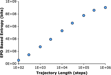
To illustrate how the trajectory plot entropy depends on constraints imposed, we examined the trajectory plot entropy as a function of trajectory length. In this case, the longer the trajectory the larger the number of different trajectories that are possible. Thus the trajectory entropy should increase with trajectory length, which it does (Fig. 7).

Fig. 7.

Quantification of trajectory plot entropy as a function of trajectory length. EPDs based on thousands of trajectories at each trajectory length are plotted as a function of trajectory length. The trajectories were from bacteria in a uniform arena of 1×10^− 9 M aspartate. From 300 steps to 100,000 steps, the trajectory plot entropy increases logarithmically (R² = 0.9998). Above 100,000 steps, the field size begins to limit the number of possible trajectories

We note that the entropy scales with the size of the image [11], but the entropy density is scale-invariant. It is also true for the k-space information in general, and chemotactic trajectories in particular, that the total information depends strongly on the size of the system. However, when properly normalized, the information density is constant. For the simulated chemotactic trajectories, this entails setting the trajectory length proportional to the arena size, and subsequently normalizing the information to the area of the arena.

Spatial information in trajectory plots depends on steepness of the gradient

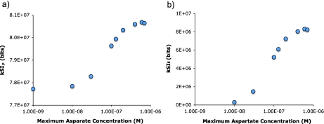
Bacterial motion is highly sensitive to the steepness of the gradient in which they are swimming [14]. The steeper the gradient the more biased their movement toward higher concentration. From the information theoretic perspective, one would expect a gradient to bias the movement of a bacterium such that an otherwise rare (high information) trajectory is more common. The steeper the gradient, the more frequent the high-information trajectories become. An examination of the average trajectory information as a function of gradient steepness shows that this is indeed the case (Fig. 8).

Fig. 8.

Spatial information increases with the steepness of an exponential gradient. Chemotaxis was simulated in exponential gradients that start at 1×10^− 9 M aspartate and end at concentrations between 1×10^− 9 and 1×10^− 6 M (in the center of the arena). The greater the end (maximum) concentration, the steeper the gradient. The information in the trajectories increased at increasingly steep gradients up to 5×10^− 7 M, which is the limit of the responsiveness with the infectivity value used (see Materials and methods). Beyond this, the receptors on the bacterium become increasingly saturated, i.e., they are saturated over an increasingly large fraction of the arena, and the information in the trajectory decreases

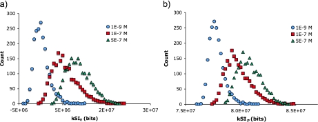
A closer examination of the distribution of the individual trajectories for any given gradient steepness shows a broad and long-tailed distribution (Fig. 9). In a set of 2,000 trajectories collected in a 1×10^− 9 M uniform arena, a small number even exceed the mean of trajectories in the 5×10^− 7 M gradient. Similarly, for a set of 2,000 trajectories collected in a 1×10^− 7 M gradient, a small number of trajectories overlap with the mean of those from the uniform arena. This type of long-tailed distribution of the trajectories is not entirely surprising, since the dynamics of flagellar activity has been shown to have a long-tailed distribution [15, 16]. Biologically, this type of behavior allows a bacterium to sometimes act in a much more biased way than if its movements were Gaussian, suggesting that there may be a benefit to occasionally making a large wager.

Fig. 9.

Variability in trajectory plot information at three different gradients (1×10^− 9 M at the bottom). a Distribution of trajectory plot kSI_E values. b Distribution of trajectory plot kSI_P values

The distribution of the kSI_P values are all positive, and because by definition I_kS ≤H_kS the kSI_P can never be negative. In contrast, the kSI_E is computed relative to some point of reference and negative values relative to that point of reference are possible (except where the point of reference is Parseval’s distribution). This property of the EPD and kSI_E is discussed further below where we discuss moving the point of reference.

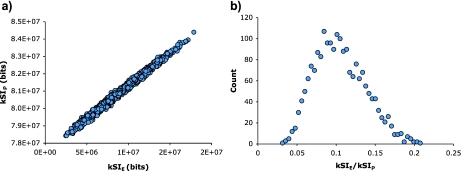
The analysis of chemotaxis in gradients produces qualitatively similar results using either the PPD or the EPD. Indeed it appears that the only difference might be an offset and scaling. However, a further examination shows that the PPD- and EPD-based results have significant differences. First, a direct comparison of the PPD and EPD values for a collection of individual trajectory plots shows that, while there is a significant correlation between the two, it is far from unity (Fig. 10). The magnitude of the differences are more easily seen in the distribution of EPD/PPD ratios, which can vary up to a factor of ∼6.

Fig. 10.

Comparison of the information in chemotactic trajectories computed using the PPD and the EPD. Graphs are based on 2,000 trajectories that were computed in an exponential gradient of 1×10^− 9 M to 5×10^− 7 M aspartate. a The kSI_P and kSI_E values show a significant correlation (R²=0.99). Yet it is clear that there is significant scatter. b The differences between the two approaches are seen more clearly in a plot of the EPD/PPD ratio. This should be ∼0.1 for perfect correlation, but varies from ∼0.03 to >0.2

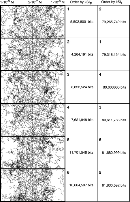
The differences between information values computed with the PPD and EPD can also be seen when a collection of individual trajectory plots are sorted by information (Fig. 11). The two probability distributions produce clearly different sort orders.

Fig. 11.

Comparison of sorting of selected individual trajectories from the data used in Fig. 10 based on kSI_P and kSI_E. The individual trajectories are sorted based on their kSI_P values. When doing so, one finds that the kSI_E values are not in the same order

Dependence of trajectory information on trajectory length

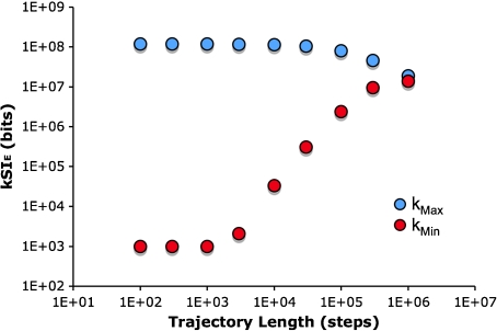
The relationship between spatial information and trajectory length was examined (Fig. 12). Taking bacteria in a 1×10^− 9 to 5×10^− 7 M exponential gradient as an example, in a k_max arena the information starts high and becomes smaller as the trajectory becomes longer. This is because the uniform background of the arena initially contributes a large amount to the information, but as an increasing fraction of the arena is visited, that contribution decreases. The converse is true for the k_min arena, where the background information is ∼0 and the trajectory adds information. The information from the two arena types converge as the trajectories approach the limit where every point in the arena has been visited at least once.

Fig. 12.

Trajectory length dependence of the spatial information for a bacterium in a 1×10^− 9 to 5×10^− 7 M exponential gradient of aspartic acid. The k_Min and k_Max arenas provide opposite points of reference

The EPD and arbitrary points of reference

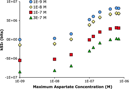
One useful property of the EPD is that information can be calculated from arbitrary points of reference. In the above examples a uniform arena of 1×10^− 9 M aspartate was used as the point of reference, but one could just as well have used any condition, such a gradient of aspartate, to serve as a point of reference. To illustrate this point, EPDs were produced for bacteria in exponential gradients starting and 1×10^− 9 M and ending at 1×10^− 9 M, 1×10^− 7 M or 3×10^− 7 M (Fig. 13). Here the information for trajectories from conditions that are the same as those from which the EPD is computed should be 0. Thus, a trajectory from a gradient of 1×10^− 9 M to 1×10^− 7 M would have ∼0 information if the EPD was computed from those conditions. In this case, trajectories that are from less steep gradients actually have a negative information.

Fig. 13.

Effect of changing the point of reference on gradient-dependent information in chemotaxis. The same data as in Fig. 8 was used with EPDs computed at 1×10^− 9 M, 5×10^− 8, 1×10^− 7 M or 3×10^− 7 M. The 1×10^− 9 M gradient reproduces the data from above (Fig. 8), and is included for the sake of comparison

Negative information is something that Shannon eliminated in his initial postulates for quantifying information [10], but this is because he effectively used one of the limits as the point of reference. Here, because we can move the point of reference, negative values become possible. One way to rationalize this is to first consider that there is some unbiased probability distribution for all possible chemotactic trajectories (which we estimate using the uniform 1×10^− 9 M aspartate arena). An EPD such as the one from 1×10^− 9 M to 1×10^− 7 M trajectories is constructed from a biased subset of trajectories. Thus, positive information means that the trajectory is rare relative to the unbiased probability distribution and rare relative to biased one. A negative information, on the other hand, means that the trajectory is common in the unbiased distribution of all trajectories, but rare in the biased distribution.

Conclusions

Living organisms commonly respond to changes in their environment by altering the direction of motion, and the path an organism takes can be viewed as a spatial manifestation of information it has gathered from the environment. Bacterial chemotaxis is one of the most well-studied examples of such a process, and the swimming trajectories of chemotaxing bacteria in response to a variety of stimuli have been extensively studied [1]. Bacterial chemotaxis is typically quantified as a biased diffusion, where the net rate of movement toward the source of a chemoattractant is used as a figure of merit. However, this assumes that the bias in a trajectory produces a net directional movement over time, and usually involves pre-judging the direction of movement. From an informational point of view, the issue is not: how quickly does a bacterium reach some particular position, or even how quickly does it move in any direction. The question is: how biased is the movement of a cell in the presence versus the absence of the external signal? A more general method for quantifying bias in movement has been described for chemotaxing Dictyostelium, where the distribution of pointing angles for a trajectory can be used to compute an information entropy [7, 8]. This, however, leaves open the possibility of some results that do not make any sense. For example, the angle-based information entropy for a perfect circle is identical to that for a random walk.

In the present work, we developed a new approach to computing the information in chemotactic trajectories that overcomes these limitations and has broad utility for a range of data that takes the form of a trajectory or path. We began by showing that the original k-space formalism based on Parseval’s distribution [11] can be used to quantify information in graphical representations of the trajectories of chemotaxing bacteria. In particular, responses to gradients of aspartic acid can be measured. However, the Parseval’s based probability distribution does not account for physical constraints on the trajectory such as the requirement of connectivity between points along the path. To address this issue, we extended the k-space formalism and showed that a well-converged experimental probability distribution for the Fourier coefficients from a chemotactic trajectory can be computed with relatively modest effort. This EPD can then be used to compute a measure of the spatial information for the information represented in trajectories of a chemotaxing bacterium in a manner that accounts for any constraint that biases a trajectory. The EPD can be computed for any reference state desirable, and the information for trajectories computed is relative to that state. The EPD also provides a measure of total trajectory space available. This novel aspect of the EPD should be applicable to a wide range of problems beyond trajectories, such as quantifying conformational space for polymers.

Another important point is that the spatial information computed here is agnostic with respect to the source of the chemoattractant; it reflects only the extent to which a trajectory is biased away from common trajectories. This is unlike measures that depend on knowing the position of sources or sinks of chemoattractants or some point toward which movement is occurring [4, 17]. The distinction here is that the question of how much information is in the trajectory is, strictly speaking, separate from what might be useful or correct information. Further, the k-space information metric is easily and directly applied to situations where there are multiple gradients that interact in complicated ways. A simple progress variable such as biased diffusion is not useful in those types of settings.

We also showed that information values calculated based on Parseval’s distribution and the experimental probability distributions have a high degree of covariance, but that they differ. It is likely that the PPD will be an adequate approximation for many types of problems, while the EPD will be required as the system becomes increasingly constrained. Finally, we note that the methods developed here are quite general, and, like the PPD, the EPD can be applied to any data object for which a Fourier transform can be computed. With respect to trajectory analysis, it would appear that a wide range of trajectory types, ranging from learning in mice [18] to neuronal pathfinding [19] and migration patterns of whales [20], could benefit from the information-based analysis presented here.

References

- 1.Berg HC. E. coli in Motion. New York: Springer; 2004. [Google Scholar]
- 2.Falke JJ, Bass RB, Butler SL, Chervitz SA, Danielson MA. The two-component signaling pathway of bacterial chemotaxis: a molecular view of signal transduction by receptors, kinases, and adaptation enzymes. Annu. Rev. Cell Dev. Biol. 1997;13:457–512. doi: 10.1146/annurev.cellbio.13.1.457. [DOI] [PMC free article] [PubMed] [Google Scholar]
- 3.Bray D, Levin MD, Lipkow K. The chemotactic behavior of computer-based surrogate bacteria. Curr. Biol. 2007;17:12–19. doi: 10.1016/j.cub.2006.11.027. [DOI] [PubMed] [Google Scholar]
- 4.Vladimirov N, Lovdok L, Lebiedz D, Sourjik V. Dependence of bacterial chemotaxis on gradient shape and adaptation rate. PLoS Comput. Biol. 2008;4:1000242. doi: 10.1371/journal.pcbi.1000242. [DOI] [PMC free article] [PubMed] [Google Scholar]
- 5.Alt W.Biased random walk models for chemotaxis and related diffusion approximations J. Math. Biol. 19809147–177.6614240434.92001 10.1007/BF00275919 [DOI] [PubMed] [Google Scholar]
- 6.Zonia L, Bray D. Swimming patterns and dynamics of simulated Escherichia coli bacteria. J. R. Soc. Interface. 2009;6(4):1035–1046. doi: 10.1098/rsif.2008.0397. [DOI] [PMC free article] [PubMed] [Google Scholar]
- 7.Andrews BW, Iglesias PA.An information-theoretic characterization of the optimal gradient sensing response of cells PLoS Comput. Biol 2007315323693672007PLSCB...3..153A 10.1371/journal.pcbi.0030153 [DOI] [PMC free article] [PubMed] [Google Scholar]
- 8.Fuller D, Chen W, Adler M, Groisman A, Levine H, Rappel W-J, Loomis WF.External and internal constraints on eukaryotic chemotaxis Proc. Natl. Acad. Sci. USA 20101079656–9659.2010PNAS..107.9656F 10.1073/pnas.0911178107 [DOI] [PMC free article] [PubMed] [Google Scholar]
- 9.Shannon CE.A mathematical theory of communication Bell Syst. Tech. J. 194827379–423.262861154.94303 [Google Scholar]
- 10.Heinz WF, Werbin JL, Lattman E, Hoh JH. Computing spatial information from Fourier coefficient distributions. J. Membr. Biol. 2011;241:59–68. doi: 10.1007/s00232-011-9362-x. [DOI] [PubMed] [Google Scholar]
- 11.Berg HC, Brown DA.Chemotaxis in Escherichia coli analysed by three-dimensional tracking Nature 1972239500–504.1972Natur.239..500B 10.1038/239500a0 [DOI] [PubMed] [Google Scholar]
- 12.Berg HC, Brown DA. Chemotaxis in Escherichia coli analyzed by three-dimensional tracking. Antibiot. Chemother. 1974;19:55–78. doi: 10.1159/000395424. [DOI] [PubMed] [Google Scholar]
- 13.Freedman D, Lane D.The empirical distribution of Fourier coefficients Ann. Stat. 198081244–1251.5946410449.62036 10.1214/aos/1176345197 [DOI] [Google Scholar]
- 14.Macnab RM, Koshland DEJ.The gradient-sensing mechanism in bacterial chemotaxis Proc. Natl. Acad. Sci. USA 1972692509–2512.1972PNAS...69.2509M 10.1073/pnas.69.9.2509 [DOI] [PMC free article] [PubMed] [Google Scholar]
- 15.Korobkova E, Emonet T, Vilar JM, Shimizu TS, Cluzel P.From molecular noise to behavioural variability in a single bacterium Nature 2004428574–578.2004Natur.428..574K 10.1038/nature02404 [DOI] [PubMed] [Google Scholar]
- 16.Emonet T, Cluzel P.Relationship between cellular response and behavioral variability in bacterial chemotaxis Proc. Natl. Acad. Sci. USA 20081053304–3309.2008PNAS..105.3304E 10.1073/pnas.0705463105 [DOI] [PMC free article] [PubMed] [Google Scholar]
- 17.Vergassola M, Villermaux E, Shraiman BI.‘Infotaxis’ as a strategy for searching without gradients Nature 2007445406–409.2007Natur.445..406V 10.1038/nature05464 [DOI] [PubMed] [Google Scholar]
- 18.Spink AJ, Tegelenbosch RA, Buma MO, Noldus LP. The ethovision video tracking system—a tool for behavioral phenotyping of transgenic mice. Physiol. Behav. 2001;73:731–744. doi: 10.1016/S0031-9384(01)00530-3. [DOI] [PubMed] [Google Scholar]
- 19.Raper JA, Bastiani M, Goodman CS. Pathfinding by neuronal growth cones in grasshopper embryos. I. Divergent choices made by the growth cones of sibling neurons. J. Neurosci. 1983;3:20–30. doi: 10.1523/JNEUROSCI.03-01-00020.1983. [DOI] [PMC free article] [PubMed] [Google Scholar]
- 20.Laidre KL, Heide-Jorgensen MP, Logsdon ML, Hobbs RC, Dietz R, VanBlaricom GR. Fractal analysis of narwhal space use patterns. Zoology (Jena) 2004;107:3–11. doi: 10.1016/j.zool.2003.09.001. [DOI] [PubMed] [Google Scholar]