Structural Equation Modeling Highlights the Potential of Kim-1 as a Biomarker for Chronic Kidney Disease

Abstract

Background

Chronic kidney disease (CKD) is a major public health problem, and despite continued research in the field, there is still a need to identify both biomarkers of risk and progression, as well as potential therapeutic targets. Structural equation modeling (SEM) is a family of statistical techniques that has been utilized in the fields of sociology and psychology for many years; however, its utilization in the biological sciences is relatively novel. SEM's ability to investigate complex relationships in an efficient, single model could be utilized to understand the progression of CKD, as well as to develop a predictive model to assess kidney status in the patient.

Methods

Fischer 344 rats were fed either an ad libitum diet or a calorically restricted diet, and a time-course study of kidney structure and function was performed. EQS, a SEM software package, was utilized to generate five CKD models of the Fisher 344 rat and identify relationships between measured variables and estimates of kidney damage and kidney function.

Results

All models identified strong relationships between a biomarker for CKD, kidney injury molecule-1 (Kim-1) and kidney damage, in the Fischer 344 rat CKD model. Models also indicate a strong relationship between age and renal damage and dysfunction.

Conclusion

SEM can be used to model CKD and could be useful to examine biomarkers in CKD patients.

Introduction

Chronic kidney disease (CKD) is a major public health problem due to its high prevalence; its association with high mortality, high morbidity, and low quality of life [1,2,3,4,5]. Despite much recent effort and research in the field of CKD, there remains a need for improvements in therapeutics and identifying and/or predicting patient outcomes. In addition, there is a great need for earlier identification and awareness of CKD, as only 3–5% of patients with stages 1–3 are aware that they have kidney disease [6]. Eddy and Neilson [7] indicate two main areas to be addressed, the need to identify both at-risk and early-stage patients and to develop more effective treatment approaches to combat CKD.

Structural equation modeling (SEM) is a ‘family of powerful and flexible statistical techniques for examining complex research questions’ and analyzing the relationships between multiple variables [8,9]. The basic concept of SEM is to design a hypothesized model of relationships between variables and then evaluate if the experimental data supports that model. SEM has two key parts: the measurement model, which defines the relationships between measurable variables and non-measurable latent factors, and the structural model, which delineates the path links and coefficients between and among the latent variables [10]. SEM has some major advantages as compared to other statistical techniques: (1) it allows for the examination of complex, multivariate questions beyond simple correlations among single sets of variables, and (2) it is not limited by measurable variables, but it allows for the utilization of latent factors, i.e. factors that cannot be measured or observed on their own, but that can be expressed by measurable variables [11]. This advantage adds an increased level of sophistication in examining complex relationships. In addition, SEM is able to accurately measure unreliable events because it is able to define and quantify an error measurement that is indicative of errors, such as biological variance and errors in data acquisition. While most datasets are imperfect, SEM is unique in its ability to compensate for this issue; other statistical approaches such as multiple regression and observed variable path analyses are unable to account for these flaws [11].

A measurement model defining relationships between measurable variables and latent factors is created, and then a step-by-step process is implemented to assess and fine-tune the model through the addition of relationships between latent variables. The model is examined using the SEM software package to evaluate how well the hypothesized model reflects the data. An iterative procedure is used to estimate model parameters, such as covariances, variances, and coefficients of regression that is guided by the decrease in the value of the difference between the observed covariance matrix and the theoretical covariance matrix computed from the parameters in the model [9]. The adjustments continue by the iterative process until the predictive values converge towards the observed true values of the parameter [9]. Once convergence occurs, the model is evaluated using both statistical and theoretical tests.

Although SEM has been utilized in the fields of sociology and psychology for many years, its use in the biological sciences is relatively novel, but recognized [12]. Research in the field of CKD has advanced far beyond examination among variables of simple correlations. The pathophysiology of the disease is complicated, involving an interplay of cardiovascular and renal factors. Thus, there is a pressing need to be able to examine these complex relationships and interactions. SEM could generate a CKD model that identifies novel biomarkers and potential therapeutic targets. Ultimately, SEM could be utilized to create a predictive, bedside model that would allow the physician to plug in measurable values and glean information about the patient's current renal status and prognosis. Ultimately this information would be valuable in the prevention and management of CKD.

Methods

Animals

Male Fischer 344 rats were fed an ad libitum (AL) diet; this is an established model of chronic renal dysfunction [13] that has been used by our laboratory [14,15]. Importantly, age-dependent alterations in renal structure and function can be attenuated by lifelong caloric restriction (CR) [16]; this adds an additional control for this model. In this model, renal dysfunction occurs between 18 and 24 months [17,18]. A time-course study was utilized to examine age-related structural and functional changes in the kidneys of rats between the ages of 4 and 24 months. In addition, there was a 24-month-old CR group of Fischer 344 rats that was fed a CR diet. CR was initiated with a 10% CR at 10 weeks until 15 weeks, and then increased to 25–40% restriction. Metabolic cages were utilized to collect 24-hour urine for measurements of urine volume, albumin (commercially available kit from BioAssay Systems), and kidney injury molecule-1 (Kim-1) [19]. Animals were anesthetized with 87 mg/kg ketamine and 13 mg/kg xylazine, then weighed, and sacrificed. Blood collection was by cardiac puncture once the abdominal cavity was opened. Blood was centrifuged 300 g for 15 min at 4°C. BUN was measured with a commercially available kit (BioAssay Systems), which utilizes a chromogenic reagent that forms a colored complex in the presence of urea. Serum creatinine was measured with a commercially available kit (BioAssay Systems) based on picrate forming a red-colored complex with creatinine. Kidneys were removed and renal structure was assessed by blind histological evaluation in which kidney tissues were examined and scored from 0 to 4 (0 = normal; 4 = extensive damage) for glomerulosclerosis (GS) and tubular damage. For these studies, animals were purchased from the NIA at the different ages and sacrificed within 1 week of arrival; all assays were performed simultaneously for all samples. All animal studies were in compliance with the guidelines for animal welfare regulations and conformed to institutional standards.

Data Analysis

SEM was performed utilizing EQS 6.1 for Windows (Multivariate Software, Inc.), to compare the proposed, hypothetical model with the set of data from the Fischer 344 rat. Through a step-by-step process using EQS, a CKD predictive model of the Fischer 344 CKD rat data was generated. Variables that were evaluated for use in the model included body weight, kidney weight, kidney to body weight ratio, urine volume, BUN, serum creatinine, creatinine clearance, urine creatinine, urine albumin, ratio of urine albumin to urine creatinine total urine protein, Kim-1, ratio of Kim-1 to urine creatinine, GS, and tubular damage (table 1). Based on preliminary inspection of the data, several variables including albumin, Kim-1, albumin/creatinine and Kim-1/creatinine were found to have a log-normal distribution; accordingly, the logarithm (base 10) of these variables was used in the analyses. Prior to modeling, variance inflation factors (VIF) of the variables were computed to detect potential multicollinearity, which occurs when there is a strong linear correlation among the predictor variables. When these are highly correlated, it becomes difficult for the model to determine which predictor(s) is (are) affecting the response. Variables having VIF values >10 were removed from consideration, except for the albumin/creatinine ratio (ACR) which was included in two models for comparison, despite having marginal to high VIF values (table 2). Covariance matrices were constructed from the variables and used as input for the analysis [20].

Table 1.

The impact of age on renal structural and functional indices in male Fischer 344 rats

	Age, months
	4	8	12	18	24	24-CR
Body weight, g	345 ± 7	379 ± 16	409 ± 7	427 ± 14	421 ± 9	315 ± 6
BUN, mg/dl	26.6 ± 2.3	21.8 ± 2.3	22.7 ± 3.5	28.9 ± 4.4	50.0 ± 3.8	31.3 ± 4.5
Creatinine clearance, ml/min/g kidney	2.61 ± 0.05	2.29 ± 0.41	2.68 ± 0.73	2.48 ± 0.84	0.970 ± 0.228	1.98 ± 0.34
GS	0.00 ± 0.00	0.50 ± 0.29	1.00 ± 0.00	1.25 ± 0.25	3.5 ± 0.29	0.5 ± 0.29
Kidney weight, g	2.29 ± 0.05	2.42 ± 0.19	2.58 ± 0.08	2.84 ± 0.05	3.43 ± 0.31	2.24 ± 0.08
Kidney/body weight, ×103	6.63 ± 0.06	6.35 ± 0.29	6.31 ± 0.16	6.70 ± 0.35	8.16 ± 0.80	7.09 ± 0.19
Kim-1, pg/ml	124 ± 3	114 ± 2	146 ± 19	234 ± 27	962 ± 632	147 ± 33
Kim-1/creatinine, μg/g	5.33 ± 0.54	5.33 ± 0.40	5.49 ± 0.87	12.5 ± 1.7	173 ± 239	27.6 ± 5.3
Serum creatinine, mg/dl	0.693 ± 0.021	0.847 ± 0.123	0.829 ± 0.258	0.934 ± 0.286	2.23 ± 0.61	0.987 ± 0.175
Total protein, mg/dl	2.00 ± 0.12	1.65 ± 0.09	2.42 ± 0.35	2.24 ± 0.29	5.94 ± 1.18	0.938 ± 0.262
Tubular damage	0.50 ± 0.29	1.25 ± 0.25	1.00 ± 0.00	1.25 ± 0.25	3.25 ± 0.48	0.25 ± 0.25
Urine albumin, mg/dl	7.36 ± 0.16	5.97 ± 0.22	21.5 ± 3.5	16.6 ± 3.6	125 ± 29	9.18 ± 1.42
Albumin/creatinine, g/g	3.17 ± 0.30	2.80 ± 0.18	8.08 ± 1.28	8.87 ± 2.00	225 ± 132	17.3 ± 2.4
Urine creatinine, μmol/kg/days	6.00 ± 0.40	5.55 ± 0.34	5.96 ± 0.17	5.26 ± 0.41	3.31 ± 0.55	2.99 ± 0.37
Urine volume, ml/day	10.1 ± 1.0	11.3 ± 1.3	10.4 ± 0.2	13.5 ± 0.9	28.8 ± 6.2	19.6 ± 1.2

Male Fisher 344 rats were fed an AL diet or a CR diet. Time course study was performed to assess functional and structural damage. Rats fed the AL diet were evaluated at 4, 8, 12, 18, and 24 months (4-, 8-, 12-, 18-, and 24-AL); rats fed the CR diet were evaluated at 24 months (24-CR). Each value represents the mean ± SE from 4 animals. To more accurately represent the center and spread of values for Kim-1, Kim-1/creatinine, urine albumin and albumin/creatinine, means were calculated from the log¹⁰ transforms; the antilog of the mean is shown in the table. Standard errors for these variables were approximated as the antilog of the margin of error for 95% confidence intervals around the log-transformed means. Functional parameters of the kidney were measured, including blood urea nitrogen (BUN), serum creatinine, urinary albumin, and creatinine clearance. The 24-AL group had the greatest impairment of function, which was corrected in the 24-CR group. Structural damage was assessed by blind histological evaluation, in which a score between 0 and 4 was given for glomerulosclerosis (GS) and tubular damage (0 = normal and 4 = extensive damage). GS and tubular damage were high in the 24-AL group, but were back to baseline in the 24-CR group.

Table 2.

Variance inflation factors (VIFs) for predictor variables in models

Variable	Model
	1	2	3	4	5
Alb/Cr	–	–	10.10	13.24	–
UAlb	5.57	4.89	–	–	–
BUN	2.57	2.97	3.44	3.38	2.86
CreatCl	2.97	2.68	3.22	3.09	3.27
GlomScl	5.1	5.93	7.14	7.05	5.25
Kim-1/Cr	–	5.01	–	8.16	–
Kim-1	4.81	–	5.25	–	6.84
SCreat	6.35	6.61	6.17	6.65	6.15
TotProt	–	–	–	–	6.37
TubDamage	4.11	4.89	5.41	4.96	7.04
UCreat	–	–	–	–	3.00

VIFs are measures of multicollinearity in model predictor variables. Although there are no mutually agreed upon limits to VIF, values >10 indicate high multicollinearity. There was an acceptable degree of multicollinearity in models 1, 2 and 5. The VIF value for the albumin/creatinine ratio (Alb/Cr) was marginal in model 3 and high in model 4.

Exploratory factor analysis was performed initially to determine how many latent variables would be needed to explain the variance and covariance among the observed measures. The observed variables were then associated with the latent variables based on the factor loading analysis to establish initial models. Lagrange multiplier or Wald tests were used as necessary to respecify the initial model. The Lagrange multiplier (LM statistic) helps to determine the overall effect of adding new relationships (variances or covariances) to the model, while the Wald test can indicate which parameters should be removed to improve the fit. Through the step-by-step process, the model generated was determined to be a valid, good-fitting model of the rat data based on both a statistical evaluation of classical SEM parameters of overall fit values and a theoretical evaluation. Model parameters and coefficients generated in the EQS package were confirmed identical to those obtained with LISREL (version 8.80; Scientific Software Int.) and AMOS (version 17.0.0; Amos Development Corp.).

Results of the final models were used to generate a set of factor score weights that are the regression coefficients estimated for predicting a latent variable from a set of observed variables. These coefficients were then used to calculate an index for each latent variable (i.e. kidney damage and kidney function) as a weighted sum of the corresponding observed variables. Latent variable indices were computed for each rat and then averaged for each age group. The ratio of the average latent score for damage to the average latent variable score for function was also calculated.

Results

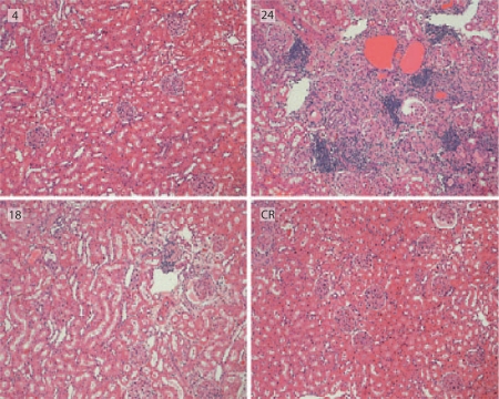
The aged AL rats (24-month AL) showed characteristics analogous to those seen in the CKD. A dramatic increase in urine volume was seen in the 24-month AL rats as compared to 4- to 18-month AL rats; this finding is supported by presence of polyuria in CKD [21] (table 1). Kidney function was assessed by BUN, serum creatinine, urine albumin, and creatinine clearance (table 1). BUN, serum creatinine, and urine albumin were all significantly higher in 24-month AL rats, while creatinine clearance was significantly decreased. Changes in BUN, serum creatinine, urine albumin, and creatinine clearance were prevented in the 24-month CR rats (24-month CR). The average blinded histology scores of the 24-month AL for GS and tubular damage were higher than those of the 4- to 18-month AL rats, and inflammation and tubulointerstitial fibrosis were noted in the 24-month AL as compared to the other groups (fig. 1). Interestingly, the functional and structural changes seen in the 24-month AL group were not observed in the 24-month CR group (table 1).

Fig. 1.

Structural indices of male Fisher 344 rats. Sections shown here are from the 4-month AL group (4), from the 18-month AL group (18), from the 24-month AL group (24), and from the 24-month CR group (CR). Tubulointerstitial fibrosis and inflammation were evident in the 24-AL group, but not present in the CR group.

Using SEM, five latent variable path models of CKD in the Fischer 344 rats were created. All models were determined to be valid and fit the data well, both statistically and theoretically. Statistically, the classical SEM parameters of the model are consistent with those of a good-fitting SEM model (table 3). The χ² (normal theory weighted) and p value test the null hypothesis that the covariance matrix for the observed parameters estimated from the model is equal to the covariance matrix for the observed parameters computed from the data. A non-significant p value indicates a good model. The root mean square error of approximation (RMSEA) [22] is now considered one of the most informative criteria in evaluating a covariance structure model [23]. The RMSEA measures the discrepancy between a model with optimal parameters and the current model. RMSEA is sensitive to the complexity of the model as well as the goodness of fit. Values <0.05 indicate a good fit [4,5]. The expected cross validation index (ECVI) was created as a means for assessing the likelihood that a model would cross-validate across similar samples from the population [24]. ECVI can take on any value, but models having smaller ECVI values are considered to have the greater potential for replication. The rank order of ECVI values is generally similar to that of AIC or CAIC. The standardized root mean square residual (Std. RMR) is another metric for evaluating the difference between the covariance matrix of the model and the covariance matrix of the data. The standardized RMR ranges from 0 to 1, and is small (<0.05) in well-fitting models. The goodness of fit index (GFI) is commonly reported in the SEM literature, although the comparative fit index (CFI) is considered one of the best indices of fit. Values >0.90 for GFI and >0.95 for the CFI indicate acceptable fits to the data [9]. Aikaike's information criterion [25] and the consistent AIC (CAIC) [26] seek to balance goodness of fit against excessive model complexity. Models with the lowest AIC or CAIC are preferred.

Table 3.

Indices for evaluating goodness of fit of models

Fit index	Model
	1	2	3	4	5
DF	12	11	10	10	10
χ2	8.44	9.76	6.33	7.99	0.79
p value	0.750	0.552	0.787	0.630	>0.999
RMSEA	<0.001	<0.001	<0.001	<0.001	<0.001
ECVI	1.91	1.96	2.00	2.00	2.70
Std. RMR	0.030	0.040	0.046	0.047	0.014
GFI	0.91	0.89	0.93	0.91	0.99
CFI	1.00	1.00	1.00	1.00	1.00
AIC	40.4	43.8	42.3	44.0	52.8
CAIC	75.3	80.8	81.5	83.2	109.4
Mean VIF	4.50	4.71	5.82	6.65	5.10

Based on the indices in table 2, models 1 through 5 all provide acceptable fits to variance-covariance relationships of the observed data. The numbering of the models is based on their CAIC rank, with model 1 being considered most acceptable and model 5 least acceptable. Measures such as the CAIC evaluate both fit and parsimony. Although model 5 technically provides the best fit to the data (based on estimates of the χ², standardized RMR, and GFI), it does so at the expense of model complexity. Model 5 includes 36 parameters (10 variances, 8 covariances, and 18 factor weights), whereas model 1 requires only 24 parameters (9 variances, 1 covariance, and 14 factor weights) to provide a satisfactory fit to the data.

Theoretically, the models were evaluated to determine if they appeared appropriate and logical based on current knowledge of some of the known relationships of CKD. Importantly, previously known relationships in CKD, i.e. serum creatinine and albuminuria, were also identified by our SEM models.

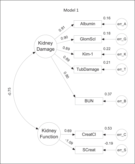
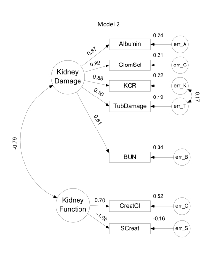
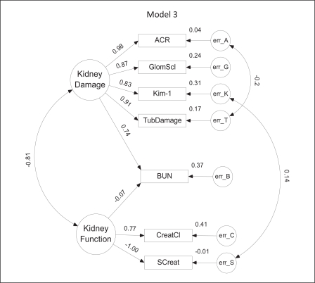
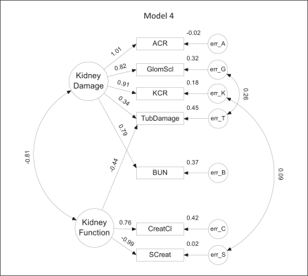
The SEM models for CKD are depicted diagrammatically in figures 2, 3, 4, 5, 6. Parameter values depicted in each diagram correspond to the completely standardized solution of the models. In these diagrams, unobserved or latent factors are represented by large circles while the observed or measurable variables are represented by rectangles. Small circles (labeled err) represent residual errors. Single-headed straight arrows symbolize direct relationships between variables, whereas curved double-headed arrows represent covariances. Values shown to the left of each observed variable represent the (standardized) level of influence of the latent factor upon that variable; values to the upper right of each observed variable depict the standardized value of the error variance.

Fig. 2.

Model 1. The Fischer 344 CKD model generated from SEM studies. Large circles represent latent factors, which are unobserved variables and include the factors, function and damage. Rectangles represent variables that can be observed or directly measured. Single arrows represent a one-directional effect from one variable to another, while dual-head arrows represent factor covariances. Standardized path coefficients are indicated by the numbers above the arrows and represent the correlation or strength of the relationship between factors. A negative coefficient represents an inverse relationship between the variables, while a positive coefficient represents a direct relationship. Small circles (labeled err) represent variance in each observed variable that cannot be accounted for by the model, such as biological variability and measurement error. The magnitude of the error variance is indicated to the upper right of each observed variable. This model was ranked first based on the CAIC, indicating the most favorable balance between fit and complexity. Unlike models 2 through 5, the model includes only a single covariance–that between the latent variables.

Fig. 3.

Model 2. This model differs from model 1 in the substitution of the Kim-1/creatinine ratio (KCR) in place of Kim-1, and in the inclusion of an error covariance between the Kim-1/creatinine ratio and tubular damage (TubDamage).

Fig. 4.

Model 3. This model differs from model 1 mainly in the substitution of the albumin/creatinine ratio (ACR) for urine albumin. It also includes two additional error term covariances: between ACR and TubDamage and between Kim-1 and serum creatinine (SCreat).

Fig. 5.

Model 4. In this model, both urine albumin and Kim-1 are normalized to urine creatinine (ACR = albumin/creatinine ratio; KCR = Kim-1/creatinine ratio). Positive covariances exist between the error terms for glomerulosclerosis (GlomScl) and tubular damage (TubDamage) as well as between KCR and serum creatinine (SCreat).

Fig. 6.

Model 5. This differs from models 1 through 4 in the incorporation of total protein (TotProt) and urine creatinine (UCreat) and absence of albumin or albumin/creatinine. While best fitting, it is the most complex, incorporating not only several additional observed variables but also a total of 8 covariance links.

Values depicted on each diagram correspond to the values in the three matrices used to approximate the covariance matrix of the observed values. The observed data are placed in an array X, such that each row corresponds to one of a total of n experimental subjects and each column corresponds to a measured variable. This array is then centered by subtracting the mean of each column (variable) from the individual values in the corresponding column. Let the centered data array be labeled X_c. The covariance matrix Σ of the centered data may be calculated as:

$${\displaystyle \sum ={X^{\prime }}_c{X}_c/n}$$

where X′ represents the transpose of X. This actual covariance matrix is estimated by the SEM process as:

$${\displaystyle \sum _{}^{^}={\Lambda }_x\Phi {{\Lambda }^{\prime }}_x+{\Theta }_{\delta }}$$

where Σ∘ is the covariance matrix predicted from the model, Λ_x is a matrix of path coefficients related to the latent variables, Φ is a symmetrical variance-covariance matrix among the latent factors and Θ_δ is a symmetrical variance-covariance matrix among the errors of measurement for the observed variables. It is the degree of similarity between Σ and Σ∘ that forms the basis of the various goodness of fit indices shown in table 2. For covariance prediction, these matrices would use unstandardized coefficients. However, we can illustrate the correspondence between the model equation and the SEM diagram by inserting standardized values from the diagram. Taking model 5 as an example, if the columns of the data array X were arranged in the same order as the observed variables in figure 6, the following three matrices would be obtained:

$${\Lambda }_x=\left[\begin{array}{cc}\begin{array}{l}0.90\\ 0.92\end{array}& \begin{array}{l}0\\ 0\end{array}\\ \begin{array}{l}0.90\\ 0.98\\ 0.62\\ 0.57\\ 0\\ 0\end{array}& \begin{array}{r}0\\ 0\\ -0.24\\ -0.34\\ 0.69\\ .79\end{array}\end{array}\right]$$

$$\Phi =\left[\begin{array}{l}1\\ \begin{array}{cc}-0.65& 1\end{array}\end{array}\right]$$

$$\Theta =\left[\begin{array}{llllllll}0.02\hfill & \hfill & \hfill & \hfill & \hfill & \hfill & \hfill & \hfill \\ 0\hfill & 0.15\hfill & \hfill & \hfill & \hfill & \hfill & \hfill & \hfill \\ 0\hfill & 0\hfill & 0.19\hfill & \hfill & \hfill & \hfill & \hfill & \hfill \\ 0\hfill & -0.14\hfill & -0.10\hfill & 0.04\hfill & \hfill & \hfill & \hfill & \hfill \\ 0\hfill & 0\hfill & 0\hfill & -0.07\hfill & 0.36\hfill & \hfill & \hfill & \hfill \\ 0\hfill & 0\hfill & 0\hfill & 0\hfill & 0\hfill & 0.30\hfill & \hfill & \hfill \\ 0\hfill & -0.07\hfill & 0\hfill & 0\hfill & 0\hfill & -0.26\hfill & 0.52\hfill & \hfill \\ 0.11\hfill & 0.24\hfill & 0\hfill & 0\hfill & 0\hfill & 0\hfill & 0\hfill & 0.38\hfill \end{array}\right]$$

The first column in the Λ_x and Φ matrices corresponds to the kidney damage latent variable, while the second column in Λ_x and Φ corresponds to the kidney function latent variable. Values on the main diagonal of the Θ_δ matrix are the error variances (values to the upper left of the rectangles in fig. 6); off diagonal elements are the covariances among error terms (values next to the curved arrows in fig. 6). The value −0.65 in the Φ matrix corresponds to the covariance between the damage and function latent variables.

All five models identified two unobserved or latent factors as the basis for the variations observed in the measured variables (fig. 2, 3, 4, 5, 6). These factors can be considered to correspond to the level of kidney function or kidney damage based on the direction (positive or negative) of their association with or influence upon the measurable variables. For example, in model 1 (fig. 2), an increase of 1 standard deviation (SD) in kidney damage would directly increase the measured levels of log₁₀ [urine albumin] (Albumin), glomerulosclerosis (GlomScl), log₁₀ [Kim-1] (Kim-1), tubular damage (TubDamage) and BUN by 0.8–0.91 SD, depending on the value of the coefficient. A 1-SD increase in kidney function would directly increase creatinine clearance (CreatCl) and decrease serum creatinine (SCreat) by 0.69 and 1.09 SD, respectively. In each model, there was a reasonably large negative correlation (−0.65 to −0.81) between the kidney function and kidney damage latent variables, which seems reasonable in light of the expected inverse relationship between kidney damage and kidney function. This also means that changes in either latent variable would indirectly affect the measured indicators of the other latent variable. In model 1, for example, a 1-SD increase in kidney damage would decrease CreatCl by about 0.52 SD (−0.75 × 0.69), but elevate SCreat by about 0.82 SD (−0.75 × −1.09).

Model 1 depicted in figure 2 provides the best balance between complexity and closeness of fit to the experimental data. Notably, the standardized weights between both urine albumin and Kim-1 and the damage latent variable are essentially the same as the weights for the two direct measures of pathological renal damage, GS and tubular damage. BUN was also positively correlated with kidney damage, although somewhat less than the other four measures. Creatinine clearance and serum creatinine were positively and negatively correlated with the kidney function latent variable, respectively. Residual error variances were similar in magnitude for all measured variables.

Model 2 (fig. 3) was ranked second based on the CAIC and differs from model 1 in the inclusion of normalized Kim-1 (KCR) for Kim-1. Overall, values of the regression weights, variances and covariances are similar to those in model 1, but there is an additional error covariance (−0.19) between normalized Kim-1 and tubular damage. This indicates that estimated levels of KCR may be negatively influenced by increases in tubular damage.

Substitution of the ACR for urine albumin in model 1 provided the basis for model 3 (fig. 4). Of the five variables positively associated with kidney damage, ACR had the highest regression weight (0.98). Unfortunately, ACR was also associated with a borderline VIF score. Model 3 is more complex than models 1 and 2 in the addition of a (slightly negative) link between BUN and kidney function and two error covariances: one (−0.20) between ACR and tubular damage and another between Kim-1 and serum creatinine. As in model 2, tubular damage may be negatively affecting ACR values. The positive link between Kim-1 and serum creatinine seems reasonable, given that as kidney damage increases, Kim-1 increases (0.83), kidney function decreases (−0.81) and serum creatinine increases (as it is negatively related to function). The slight decrease in the correlation between kidney damage and BUN (0.74 vs. 0.80–0.81 in models 1 and 2, respectively) appears balanced by the indirect influence of BUN on kidney damage via its negative relation to function, and the negative correlation between function and damage.

In model 4 (fig. 5), both albumin and Kim-1 are normalized to urine creatinine. Although model 4 has the same overall level of complexity as model 3, its CAIC is higher due to a slightly less optimal fit. There is a covariance between KCR and serum creatinine similar to that observed in model 3 for Kim-1 and serum creatinine as well as a positive covariance between glomerular sclerosis and tubular damage. Interestingly, in this model, weights for tubular damage are nearly equally and oppositely divided between damage and function. Although the VIF for ACR in this model is unacceptably high, it was included for comparison with related models.

Model 5 (fig. 6) differed from models 1 through 4 in the addition of urine creatinine as an observed variable and substitution of total urine protein for urine albumin. It provided a remarkably close fit to the observed data as indicated by a χ² value nearly 10-fold lower than seen for the other models, but did so at a high price in complexity. Compared with model 1, model 5 adds one more observed variable, four additional regression weights, and seven additional covariances.

These five SEM models all highlight the potential of Kim-1 (or normalized Kim-1) as a biomarker for CKD. Kim-1 levels are directly influenced by kidney damage in all models with path coefficients ranging from 0.83 in model 3 to 0.98 in model 5. Comparison of the coefficients relating kidney damage to Kim-1 (or KCR), albumin (or ACR), GlomScl, TubDamage and SCreat over all five models by one-factor ANOVA reveals no significant difference between average values for Kim-1 or KCR and those the other measures (p > 0.55). This suggests that changes in Kim-1 levels are as sensitive an indicator of renal damage in the rat as any of the other measures, including direct measures of renal pathology, such as GS and tubular damage.

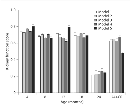
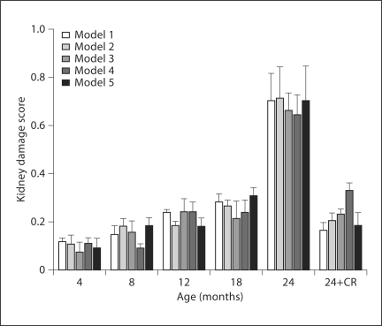
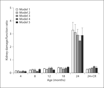
The model also permits the use of observed variables to predict the unobserved or latent variables. By multiplying the value of each observed variable by its corresponding weight, or factor score weight, we can calculate the indices of kidney function and kidney damage for the various age groups. Because latent variables are unmeasured and have no definite metric scale, their indices vary depending on scales of the observed variables. Since the number and type of observed measures varied with each model, an arbitrary common scale was applied to the computed indices to facilitate comparison. The kidneys of the aged rats (24-month AL) had severe damage and impairment of function as compared to those of the younger rats; changes in damage and function were attenuated by CR. The latent variable indices for kidney function (fig. 7) remained fairly stable in AL-fed rats at an average value of 0.71 across ages 4–18 months but dropped drastically to an average of 0.24 (66% decline) at 24 months in all models. CR rats showed a much smaller decline in function at 24 months; kidney function remained at an average of 0.61 in the 24-month CR rats, which was 86% of the level found in younger (<24 months) AL rats. In all models, the index for kidney damage (fig. 8) rose very slightly from 4 to 18 months in AL rats but rose sharply 3.8-fold above average in the 24-month AL group, representing the high level of damage to the kidneys of these aged rats. Interestingly, the index for kidney damage remained low in the 24-month CR group of rats and was only about 2% higher than the baseline observed in younger rats (0.22 vs. 0.18). The ratio of damage to function indices (fig. 9) may provide an even more sensitive indicator of renal status. The damage/function ratio remains rather stable with age in AL rats, until it jumps from an average of 0.26 to 2.93 at 24 months (fig. 9). Note, however, that it measured an average of 0.36 in the 24-month CR rats, a value not much different from that found in 12-month (0.32) or 18-month (0.38) AL groups. The latent variable indices computed from the SEM model indicate a strong relationship between increased age and kidney damage and impairment of function.

Fig. 7.

The average kidney function (latent variable) score for each group of animals in the various models. The age groups include the 4-month AL group of rats, 8-month AL group of rats, 12-month AL group of rats, 18-month AL group of rats, 24-month AL group of rats, and the 24-month CR group of rats (24-CR). Kidney function score did not change much with age in the AL group until 24 months when it decreased to less than 50% of previous values. With the exception of model 5, the function score in the 24-month-old CR rats (24+CR) was similar to that observed in younger AL rats.

Fig. 8.

The average kidney damage score for each group of animals as represented in the five SEM models. There was a gradual rise in damage in the AL group with age until 24 months, when the damage score increased sharply 3- to 4-fold. Caloric restriction (24-CR) prevented most of the rise in damage.

Fig. 9.

The ratio of the latent variable score of kidney damage to kidney function for AL-fed male Fischer 344 rats at ages 4, 8, 12, 18, and 24 months and the CR 24-month rats, represented respectively by 4-AL, 8-AL, 12-AL, 18-AL, 24-AL, and 24-CR. The damage/function ratio of the aged group of rats (24-AL) had the highest ratio in both models (over 10× values in younger rats); this was ameliorated in the aged group of CR rats (24-CR) towards baseline.

Discussion

The functional and structural changes seen in the 24-month AL rats are characteristic of renal damage and dysfunction. The 24-month AL group's structural and functional characteristics are analogous to those seen in the CKD state. The aged Fischer 344 rat is an established model of CKD [13,17,18]. In addition, since no exogenous insults were utilized to initiate CKD, this model may be considered an improved model that is more representative of the CKD state seen in humans, which is caused by more subtle insults. Despite the small sample size used in the current study, SEM is able to generate valid, good-fitting CKD models for the Fischer 344 rat. In the future, models such as this could be generated for human data and serve as predictive models to assess the current status and progression of a patient. This information would be valuable in the management of patients in treating CKD and preventing progression of the disease. SEM could generate a model to identify novel biomarkers and potential therapeutic targets. It could ultimately be utilized to create a predictive model for the patient that would allow physicians to enter measurable values and glean information about the patient's current renal status and prognosis. This information would be valuable in the prevention and management of severe CKD.

All five SEM models identify Kim-1 as a sensitive indicator of CKD in the rat. Kim-1 is a type 1 transmembrane protein that has previously been shown to be a urinary biomarker for acute tubular injury in patients as it is shed and can be measured in the urine [27]. Further studies should be done to assess whether this holds true clinically. However, our finding is supported by some emerging data suggesting that Kim-1 may be elevated in CKD. Kim-1 has been found by two independent laboratories to not only be increased in patients with immunoglobulin A nephropathy (IgAN) as compared to controls but also to be higher with proteinuria and with more severe tubulointerstitial injury, supporting our finding of Kim-1 as a strong indicator of chronic kidney damage [28,29]. Interestingly, Kim-1 and serum creatinine were determined through multivariate analysis to be significant, independent predictors of ESRD [28]. Another study investigating congenital obstructive nephropathy, the main cause of chronic renal failure in children, determined that Kim-1 levels were associated with worsening obstruction in children with hydronephrosis due to unilateral, critical degree of ureteral stenosis [30]. Urinary Kim-1 levels were increased in patients with non-diabetic CKD with proteinuria [31], and Ko et al. [32] suggest Kim-1 as a biomarker of the AKI to CKD transition receptor 1.

Although serum creatinine is currently utilized in the field to assess kidney disease, it may not be an optimal biomarker as it is affected by many other factors not related to kidney status [33,34]. It is important to note, however, that we were unable to use a standardized assay for serum creatinine. The SEM models suggest that Kim-1 is a sensitive marker of damage in rats. Kim-1 could potentially be used as a urinary biomarker of CKD in man, allowing for early identification of CKD with a non-invasive test.

The latent variable scores of kidney damage and kidney function and the damage/function ratio generated from all five SEM models demonstrate that age is a significant determinant in the progression of CKD in Fischer 344 rat. Interestingly, the negative changes in the kidney structure and function are ameliorated in the aged rats (24-month) that were fed a CR diet. This suggests a relationship between diet and kidney disease. More studies are needed to further investigate this relationship; however, it might identify an interesting aspect of CKD that could potentially offer insight into the pathophysiology of this disease. SEM has the potential to identify novel biomarkers as well as the potential for investigating therapeutics. SEM could also be utilized to create and examine the complex interplay of cardio and renal variables that affect CKD.

Disclosure Statement

J.V.B. is a co-inventor on patents licensed by Partners Healthcare to a number of companies.

References

- 1.Coresh J, Selvin E, Stevens LA, et al. Prevalence of chronic kidney disease in the United States. JAMA. 2007;298:2038–2047. doi: 10.1001/jama.298.17.2038. [DOI] [PubMed] [Google Scholar]
- 2.Filiopoulos V, Vlassopoulos D. Inflammatory syndrome in chronic kidney disease: pathogenesis and influence on outcomes. Inflamm Allergy Drug Targets. 2009;8:369–382. doi: 10.2174/1871528110908050369. [DOI] [PubMed] [Google Scholar]
- 3.Townsend RR, Felman HI. Chronic kidney disease: past problems, current challenges, and future facets. NephSAP. 2009;8:239–243. [Google Scholar]
- 4.Okusa MD, Chertow GM, Portilla D. The nexus of acute kidney injury, chronic kidney disease, and World Kidney Day 2009. Clin J Am Soc Nephrol. 2009;4:520–522. doi: 10.2215/CJN.06711208. [DOI] [PMC free article] [PubMed] [Google Scholar]
- 5.Brosnahan G, Fraer M. Chronic kidney disease: whom to screen and how to treat. Part 1: Definition, epidemiology, and laboratory testing. South Med J. 2010;103:140–146. doi: 10.1097/SMJ.0b013e3181c99438. [DOI] [PubMed] [Google Scholar]
- 6.Berns JS, Fishbane S. Chronic kidney disease and progression. NephSAP. 2009;8:244–312. [Google Scholar]
- 7.Eddy AA, Neilson EG. Chronic kidney disease progression. J Am Soc Nephrol. 2006;17:2964–2966. doi: 10.1681/ASN.2006070704. [DOI] [PubMed] [Google Scholar]
- 8.Nelson TD, Aylward BS, Steele RG. Structural equation modeling in pediatric psychology: overview and review of applications. J Pediatr Psychol. 2008;33:679–687. doi: 10.1093/jpepsy/jsm107. [DOI] [PubMed] [Google Scholar]
- 9.De Marco G, Vrignaud P, Destrieux C, de Marco D, Testelin S, Devauchelle B, Berquin P. Principle of structural equation modeling for exploring functional interactivity within a putative network of interconnected brain areas. Magn Reson Imaging. 2009;27:1–12. doi: 10.1016/j.mri.2008.05.003. [DOI] [PubMed] [Google Scholar]
- 10.Collin VT, Violato C, Hecker K. Aptitude, achievement and competence in medicine: a latent variable path model. Adv Health Sci Educ. 2009;14:355–366. doi: 10.1007/s10459-008-9121-7. [DOI] [PubMed] [Google Scholar]
- 11.Kline RB. Latent variable path analysis in clinical research: a beginner's tour guide. J Clin Psychol. 1991;47:471–484. doi: 10.1002/1097-4679(199107)47:4<471::aid-jclp2270470402>3.0.co;2-o. [DOI] [PubMed] [Google Scholar]
- 12.Fisher MA, Taylor GW, West BT, McCarthy ET. Bidirectional relationship between chronic kidney and periodontal disease: a study using structural equation modeling. Kidney Int. 2011;79:347–355. doi: 10.1038/ki.2010.384. [DOI] [PMC free article] [PubMed] [Google Scholar]
- 13.Corman B, Owen R. Normal development, growth, and aging of the kidney. In: Mohr U, Dungworth DL, Capen CC, editors. Pathobiology of Aging Rats. Washington: ILSI Press; 1992. pp. 195–209. [Google Scholar]
- 14.Chen G, Bridenbaugh EA, Akintola AD, Catania JM, Vaidya VS, Bonventre JV, Dearman AC, Sampson HW, Zawieja DC, Burghardt RC, Parrish AR. Increased susceptibility of aging kidney to ischemic injury: identification of candidate genes changed during aging, but corrected by caloric restriction. Am J Physiol Renal Physiol. 2007;293:F1272–F1281. doi: 10.1152/ajprenal.00138.2007. [DOI] [PMC free article] [PubMed] [Google Scholar]
- 15.Akintola AD, Crislip ZL, Catania JM, Chen G, Zimmer WE, Burghardt RC, Parrish AR. Promoter methylation is associated with the age-dependent loss of N-cadherin in the rat kidney. Am J Physiol Renal Physiol. 2008;294:F170–F176. doi: 10.1152/ajprenal.00285.2007. [DOI] [PubMed] [Google Scholar]
- 16.Stern JS, Gades MD, Wheeldon CM, Borchers AT. Calorie restriction in obesity: prevention of kidney disease in rodents. J Nutr. 2001;131:913S–917S. doi: 10.1093/jn/131.3.913S. [DOI] [PubMed] [Google Scholar]
- 17.Van Liew JB, Davis FB, Davis PJ, Noble B, Bernards LL. Calorie restriction decreases microalbuminuria associated with aging in barrier-raised Fischer 344 rats. Am J Physiol. 1992;263:F554–F561. doi: 10.1152/ajprenal.1992.263.3.F554. [DOI] [PubMed] [Google Scholar]
- 18.Coleman GL, Barthold SW, Osbaldiston GW, Foster SJ, Jonas AM. Pathological changes during aging in barrier-raised Fischer 344 male rats. J Gerontol. 1977;32:258–278. doi: 10.1093/geronj/32.3.258. [DOI] [PMC free article] [PubMed] [Google Scholar]
- 19.Vaidya VS, Ramirez V, Ichimura T, Bobadilla NA, Bonventre JV. Urinary kidney injury molecule-1: a sensitive quantitative biomarker for early detection of kidney tubular injury. Am J Physiol Renal Physiol. 2006;290:F517–F529. doi: 10.1152/ajprenal.00291.2005. [DOI] [PubMed] [Google Scholar]
- 20.Schreiber JB. Core reporting practices in structural equation modeling. Res Social Adm Pharm. 2009;4:83–97. doi: 10.1016/j.sapharm.2007.04.003. [DOI] [PubMed] [Google Scholar]
- 21.Fukuda M, Motokawa M, Miyagi S, Sengo K, Muramatsu W, Kato N, Usami T, Yoshida A, Kimura G. Polynocturia in chronic kidney disease is related to natriuresis rather than to water diuresis. Nephrol Dial Transplant. 2006;21:2172–2177. doi: 10.1093/ndt/gfl165. [DOI] [PubMed] [Google Scholar]
- 22.Steiger JH, Lind JC: Statistically Based Test for the Number of Common Factors. Psychometric Society Annual Meeting, Iowa City 1980.
- 23.Byrne BM. Structural Equation Modeling with LISREL, PRELIS and SIMPLIS. London: Psychology Press; 1998. [Google Scholar]
- 24.Brown MW, Crudeck R. Single sample cross-validation indices for covariance structures. Multivariate Behav Res. 1989;24:445–455. doi: 10.1207/s15327906mbr2404_4. [DOI] [PubMed] [Google Scholar]
- 25.Akaike H. Factor analysis and AIC. Psychometrika. 1987;52:317–332. [Google Scholar]
- 26.Bozdogan H. Model selection and Aikaike's information criteria (AIC): the general theory and its analytical extensions. Psychometrika. 1987;52:345–370. [Google Scholar]
- 27.Han WK, Bailly V, Abichandani R, Thadhani R, Bonventre JV. Kidney injury molecule-1 (Kim-1): a novel biomarker for human renal proximal tubule injury. Kidney Int. 2002;62:237–244. doi: 10.1046/j.1523-1755.2002.00433.x. [DOI] [PubMed] [Google Scholar]
- 28.Peters HP, Waanders F, Meier E, van den Brand J, Steenbergen EJ, van Goor H, Wetzels JF. High urinary excretion of kidney injury molecule-1 is an independent predictor of end-stage renal disease in patients with IgA nephropathy. Nephrol Dial Transplant. 2011;26:3581–3588. doi: 10.1093/ndt/gfr135. [DOI] [PubMed] [Google Scholar]
- 29.Xu PC, Zhang JJ, Chen M, Lv JC, Liu G, Zou WZ, Zhang H, Zhao MH. Urinary kidney injury molecule-1 in patients with IgA nephropathy is closely associated with disease severity. Nephrol Dial Transplant. 2011;26:3229–3236. doi: 10.1093/ndt/gfr023. [DOI] [PubMed] [Google Scholar]
- 30.Wasilewska A, Taranta-Janusz K. Kim-1 and NGAL: new markers of obstructive nephropathy. Pediatr Nephrol. 2011;26:579–586. doi: 10.1007/s00467-011-1773-5. [DOI] [PMC free article] [PubMed] [Google Scholar]
- 31.Waanders F, Vaidya VS, van Goor H, Leuvenink H, Damman K, Hamming I, Bonventre JV, Vogt L, Navis G. Effect of renin-angiotensin-aldosterone system inhibition, dietary sodium restriction, and/or diuretics on urinary kidney disease: a post hoc analysis of a randomized controlled trial. Am J Kidney Dis. 2009;53:16–25. doi: 10.1053/j.ajkd.2008.07.021. [DOI] [PMC free article] [PubMed] [Google Scholar]
- 32.Ko GJ, Grigoryev DN, Linfert D, Jang HR, Watkins T, Cheadle C, Rascusen L, Rabb H. Transcriptional analysis of kidneys during repair from AKI reveals possible roles for NGAL and Kim-1 as biomarkers of AKI-to-CKD transition. Am J Physiol Renal Physiol. 2010;298:F1472–F1483. doi: 10.1152/ajprenal.00619.2009. [DOI] [PubMed] [Google Scholar]
- 33.Refaie R, Moochhala SH, Kanagasundram NS. How we estimate GFR–a pitfall of using a serum creatinine-based formula. Clin Nephrol. 2007;68:235–237. doi: 10.5414/cnp68235. [DOI] [PubMed] [Google Scholar]
- 34.Tonelli M, Manns B. Supplementing creatinine-based estimates of risk in chronic kidney disease: is it time? JAMA. 2011;305:1593–1595. doi: 10.1001/jama.2011.502. [DOI] [PubMed] [Google Scholar]