Broadly tuned response properties of diverse inhibitory neuron subtypes in mouse visual cortex

Summary

Different subtypes of GABAergic neurons in sensory cortex exhibit diverse morphology, histochemical markers, and patterns of connectivity. These subtypes likely play distinct roles in cortical function, but their in vivo response properties remain unclear. We used in vivo calcium imaging, combined with immunohistochemical and genetic labels, to record visual responses in excitatory neurons and up to three distinct subtypes of GABAergic neurons (immunoreactive for parvalbumin, somatostatin, or vasoactive intestinal peptide) in layer 2/3 of mouse visual cortex. Excitatory neurons had sharp response selectivity for stimulus orientation and spatial frequency, while all GABAergic subtypes had broader selectivity. Further, bias in the responses of GABAergic neurons toward particular orientations or spatial frequencies tended to reflect net biases of the surrounding neurons. These results suggest that the sensory responses of layer 2/3 GABAergic neurons reflect the pooled activity of the surrounding population – a principle that may generalize across species and sensory modalities.

Introduction

GABAergic interneurons make up 15-20% of all neurons in the neocortex (Feldman and Peters, 1978; Kawaguchi and Kubota, 1997; Markram et al., 2004; Peters and Kara, 1985), where they display a remarkable diversity of subtypes as defined by morphological, molecular, and biophysical features (Ascoli et al., 2008; Burkhalter, 2008). These subtypes form distinct gap-junctional networks (Beierlein et al., 2000; Hestrin and Galarreta, 2005) and play different roles in the regulation of cortical rhythms (Cardin et al., 2009; Sohal et al., 2009; Somogyi and Klausberger, 2005), plasticity (Fagiolini et al., 2004), and state-dependent activity (Gentet et al., 2010). In primary sensory cortex, different subtypes also participate in distinct synaptic subnetworks with excitatory neurons (Yoshimura and Callaway, 2005; Xu and Callaway, 2009). However, it is unclear whether the diversity of GABAergic subtypes is paralleled by differences in their responses to sensory stimuli.

In electrophysiological studies of the cerebral cortex in vivo, interneurons have typically been identified by their biophysical properties, particularly in the distinction between narrow-spiking neurons (mostly parvalbumin-positive interneurons) and broad-spiking neurons (mostly excitatory, and some interneuron classes) (McCormick et al., 1985). The orientation selectivity of layer 2/3 narrow-spiking interneurons varies between species. In the visual cortex of species with orientation columns (e.g., cats), most layer 2/3 interneurons are sharply tuned for orientation (Azouz et al., 1997; Cardin et al., 2007), although they may be of mixed tuning width in layer 4 (Usrey et al., 2003; Nowak et al., 2008; morphologically identified interneurons: Hirsch et al., 2003; Martin et al., 1983; Ahmed et al., 1997). By contrast, in species lacking orientation columns (e.g., rodents and rabbits; Dräger, 1975; Bousfield, 1977; Girman et al., 1999; Ohki et al., 2005; Van Hooser et al., 2005), narrow-spiking interneurons exhibit weak to moderate selectivity (Swadlow, 1988, Niell and Stryker, 2008). Thus, differences in layer 2/3 GABAergic neuron selectivity may be related to the degree of functional homogeneity in the population of surrounding excitatory neurons. Alternatively, differences in tuning may represent different classes of layer 2/3 GABAergic neurons that are species-specific or less prevalent in some species than others (Lauritzen and Miller, 2003). To test these hypotheses, experimental approaches are needed that can provide: (1) robust classification of multiple identified subtypes of GABAergic neurons, and (2) measurements of orientation preference in many of the neurons surrounding each GABAergic neuron.

Imaging techniques have enabled improved identification and classification of GABAergic neurons. For instance, transgenic mice that express GFP in all GABAergic neurons (Tamamaki et al., 2003) have been used in combination with calcium imaging or targeted cell-attached recordings to study the in vivo function of a more complete sample of GABAergic neurons in visual cortex. Genetically identified GABAergic neurons exhibit less selective responses than excitatory neurons (Sohya et al., 2007; Liu et al., 2009, Kameyama et al., 2010). However, previous work has not examined potential differences between the multiple immunohistochemically defined GABAergic subtypes.

To test hypotheses regarding the functional diversity of GABAergic neurons, we combined in vivo calcium imaging with postmortem immunohistochemistry in layer 2/3 of mouse primary visual cortex (V1). We examined the visual responses of three non-overlapping GABAergic neuron subtypes based on their immunoreactivity for the markers parvalbumin (PV, 21% GABAergic neurons in V1 Layer 2/3), somatostatin (SOM, 8%), and vasoactive intestinal peptide (VIP, 17%) (percentages from Xu et al., 2009), which correspond primarily to basket, Martinotti and bipolar morphologies, respectively (Celio and Heizmann, 1981; Connor and Peters, 1984; Wahle, 1993; Kawaguchi and Kubota, 1997; Xu et al., 2006). We measured the responses to different orientations and spatial frequencies and found that all identified GABAergic subtypes show broader selectivity than neighboring excitatory neurons. Furthermore, tuning observed in GABAergic neurons tended to reflect overall biases in the surrounding population, while individual excitatory neurons exhibited tuning that was almost random with respect to the overall bias. Our results suggest that inhibitory neurons in layer 2/3 of visual cortex reflect the average sensory response of the surrounding population of neurons.

Results

Visual responses in identified neurons: in vivo calcium imaging and ex vivo immunohistochemistry

We combined in vivo two-photon calcium imaging with immunohistochemistry to study the functional properties of different cell types in the visual cortex. Experiments were conducted in C57BL/6 mice, either wild-type (n = 6) or a GAD67-GFP knock-in (n = 8) that expresses GFP in all GABAergic neurons (Tamamaki et al., 2003). An approximately 300 μm diameter sphere of neurons in layer 2/3 of mouse visual cortex was bulk loaded by injection of the calcium indicator Oregon Green BAPTA-1 AM (OGB-1; Figures 1A,B; Ohki et al., 2005; Stosiek et al., 2003). OGB-1 and GFP signals were separated using different two-photon excitation wavelengths and emission filters (see Experimental Procedures; Figure S1). A piezoelectric objective Z-scanner (Figure 1A) was used to simultaneously record the fluorescence of nearly all (typically 100-200) cells in a volume spanning 150 μm × 150 μm × 45 μm at a rate of 1 Hz (Figure 1A,B; Andermann et al., 2010). This method of volume scanning also allowed post hoc correction for small (∼ 2 - 10 μm) drifts in brain position that sometimes occured during the 2 - 3 hours of recordings in each volume. We measured the changes in fluorescence (ΔF/F) in cell bodies evoked by presentation of drifting gratings with different directions or spatial frequencies (Figure 1C).

Figure 1. Three-dimensional imaging of visual response tuning in vivo.

(A)Schematic of in vivo dye injection, volume imaging, and visual stimulation setup. (B) Left panel: Overlay of OGB-1 loaded cells (gray), SR101 stained astrocytes (orange), and GFP-expressing GABAergic neurons (green) in a three-dimensional volume of cortex that was continuously imaged at a rate of 1 Hz. Right panel: Maximum intensity volume projection across depth. (C) Example of visually evoked calcium responses in individual trials (gray traces) and average of 12 trials (black trace) for one excitatory neuron (GFP- / SR101-; black circle in B). Drifting gratings were presented in 12 directions (left panel). For 3 of these directions (0°, 120° and 240°), stimuli at 7 different spatial frequencies were presented (right panel). Stimuli were presented in pseudorandom order, but time courses are shown after sorting and concatenation. See also Figure S1.

We achieved reliable correspondence between images of cells in vivo and in immunohistochemically processed sections using fiduciary markers at multiple spatial scales (from millimeters to micrometers; Experimental Procedures; cf. Knott et al., 2009). Following in vivo calcium imaging, a fixable fluorescent dextran was injected at the imaging site, which labeled a sphere of extracellular space surrounding the recording site (400-600 μm diameter; Figure 2A). After perfusion and brain fixation, we generated histological sections parallel to the in vivo imaging plane, using the headpost implant as a common reference (Figure 2B, top left panel). Sections were then stained immunohistochemically for PV, SOM, and VIP, and in vivo to ex vivo cell alignment was performed as follows: First, we visualized the fixable dextran to constrain the search for the imaging site to within a few hundred microns and a small number of ex vivo sections (Figure 2B, middle left panel). Then, we used the patterns of large radial blood vessels to further narrow the search, until a three-dimensional cellular pattern match was identified (Figures 2B and 2C). For GAD67-GFP mice, we matched the patterns of GFP-expressing neurons in vivo and ex vivo (Figure 2C, left panels). For wild-type mice, we matched the patterns of cells labeled with OGB-1 in vivo with the extracellular negative staining that surrounded cell bodies ex vivo (Figure 2C, right panels).

Figure 2. Triple-immunostaining of GABAergic neurons.

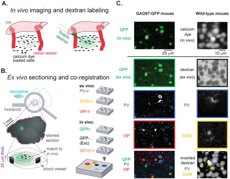
(A)Schematic in vivo cortical volume of OGB-1 labeled cells (left panel) and subsequent injection of a fixable fluorescent dextran into the extracellular space (right panel) to mark the region of imaging. (B) Schematic of ex vivo processing steps: (1) Freezing microtome sections were made parallel to the in vivo imaging plane by aligning in vivo and ex vivo brain orientation using the metal headpost used during calcium imaging (top left panel). (2) Fluorescent dextran injected in vivo (A) appeared in sections as a haze of extracellular staining ∼ 500 μm in diameter (middle left panel). Staining and vessel patterns permitted rapid localization of a pattern of cells ex vivo (bottom left panel) that matched the pattern imaged in vivo (A, left panel). (3) Up to 6 cell types were identified within a single volume by combining in vivo labeling and ex vivo immunohistochemical staining (right panels). (C) Examples of matching patterns of cells imaged in vivo and in immunohistochemical sections ex vivo. All images are maximum intensity projections across ∼20 μm in depth. In GAD67-GFP mice (left column), the pattern of GFP cells imaged in vivo was matched to the pattern of GFP cells ex vivo, while in wild-type mice (right column) the pattern of OGB-1 labeled cells in vivo was matched to the negatively stained ‘shadows’ of cells observed ex vivo that were produced by the extracellular dextran labeling. In overlay images (bottom row) individual colors were disproportionately saturated for visualization purposes. See also Figure S6E.

Using this strategy, we characterized the functional properties of a total of 216 immunohistochemically characterized GABAergic neurons, including 102 PV, 31 SOM, 33 VIP, and 50 NEG (GFP-positive, immunolabel-negative; Table 1). Of the GFP-positive GABAergic neurons that were imaged in vivo, about 85% were subsequently found ex vivo (data not shown). The remaining cells were cut between histological sections, making unambiguous identification difficult. These cells were excluded from the analyses. We also recorded the visual responses of 1,585 non-GABAergic excitatory neurons that were not labeled with either GFP or sulforhodamine 101, an astrocytic marker (see Experimental Procedures; Table 1). While the depth of recorded cells ranged from 150 μm (upper layer 2/3) to 430 μm (layer 4) below the brain surface, the majority of cells (70%) were located 200 μm to 325 μm deep (lower layer 2/3).

Table 1. Summary of cells recorded.

	Total cells*	Orientation (ΔF/F > 6%)	Spatial Freq. (ΔF/F > 6%)
Excitatory	1585	1585 (1020)	377 (281)
GABAergic	216	185 (121)	85 (59)
PV+	102	94 (74)	35 (26)
VIP+	31	25 (10)	15 (10)
SOM+	33	30 (15)	8 (6)
Negative	50	36 (22)	27 (17)

Total includes all neurons of each cell type with photon shot noise < 2% of the mean fluorescence (F). The numbers below ‘Orientation’ and ‘Spatial Freq.’ indicate the number of neurons studied with those stimulus protocols and the number that were visually responsive (in parentheses; ΔF/F > 6%). Some neurons were studied with both protocols. GABAergic neurons are from both wild-type mice (86 cells) and GAD67-GFP mice (130 cells). Excitatory neurons are only from GAD67-GFP mice and include cells that were GFP-negative and were not stained by SR101. Excitatory neurons whose preferred direction was far from any of the directions used with the spatial frequency stimulus are excluded from ‘Spatial Freq.’ (see Experimental Procedures).

^*Due to these and other criteria for inclusion (see Experimental Procedures), these numbers do not necessarily reflect the proportion of each cell type in visual cortex. See also Figure S2.

More than 60% of both excitatory and GABAergic neurons exhibited visually evoked calcium responses of sufficient magnitude for reliable estimation of tuning properties. We defined visually responsive neurons as those having > 6% ΔF/F for at least one direction/spatial frequency, as well as maximum photon shot noise < 2%, averaged over the first 4 seconds of presentation (Table 1). On average, visually responsive excitatory neurons exhibited significantly larger visually evoked calcium responses than GABAergic neurons (peak ΔF/F: 22.4 ± 0.4% vs. 16.2 ± 0.6%, p < 10^-7; mean ΔF/F in first 4 s: 16.5 ± 0.3% vs. 11.0 ± 0.4%, p < 10^-7; K-S tests, Figure S2A). This reflects the smaller calcium influx per spike in GABAergic neurons compared to excitatory neurons (see below, Figures 3C, S3G).

Figure 3. Simultaneous recordings of calcium transients and action potentials provide similar measurements of orientation selectivity.

(A)Time courses of visually evoked calcium transients (black) and spike rates (gray) in response to the presentation of oriented gratings for a putative excitatory neuron (average of 6 trials; left). Polar plot of average tuning as measured by calcium transients (black) and spike rates (gray) for this excitatory cell (right, average of 0 s to 4 s post-stimulus onset). Tick marks on polar plots: 10% ΔF/F (black) and 1.5 spikes/s (gray). (B) Same as (A) for a PV neuron (red: calcium transients; gray: spike rates, average of 12 trials; left). Tick marks on polar plots: 4% ΔF/F (red) and 7 spikes/s (gray). (C) Comparison of the mean calcium transient evoked and the simultaneously measured spike rate for all recorded excitatory (left, black lines, mean ± SEM) and PV neurons (right, red lines). Only bins containing >4 trials are shown. Note the linearity of the relationship between calcium transients and spike rate and the higher spike rates recorded in the PV neurons. Firing rates above the transition from a solid to dashed line account for <15% of total spikes recorded. (D) Plot of orientation selectivity as measured simultaneously with calcium transients and spike rates. All values lie near the unity line. See also Figure S3.

An especially high proportion of PV neurons were visually responsive. The proportion of PV neurons responsive to the orientation protocol (79%, 74 of 94 PV neurons) was significantly greater than that of all other GABAergic subtypes (VIP: 40%, 10 of 25, p < 10^-3; SOM: 50%, 15 of 30, p < 0.01; NEG: 61%, 22 of 36, p < 0.05; Table 1). VIP neurons exhibited both the lowest proportion responsive and significantly smaller magnitude responses than the other GABAergic subtypes (peak ΔF/F: 11.4 ± 0.8% vs. 16.6 ± 0.7%, p < 0.05; K-S tests, Figures S2A and 4B). Visual stimuli may elicit very few spikes in this subtype, although it is also possible that the calcium influx per spike is substantially lower than the other GABAergic subtypes.

Calcium responses reflect the spiking activity, and tuning, of excitatory and PV GABAergic neurons

In a series of electrophysiological control experiments, we validated the use of calcium transients to estimate the selectivity of visually evoked responses. Previous work demonstrated a linear relationship between somatic fluorescence signal and in vivo spontaneous spiking in rat cortical neurons (OGB-1, Kerr et al., 2005). However, linearity in cortical excitatory neurons at the high firing rates evoked by visual stimulation was unclear (up to 6 Hz average firing over 4 seconds; Figure 3C, left panel). Further, the in vivo relationship between spiking and fluorescence changes in cortical GABAergic neurons was unknown (although linear in zebrafish GABAergic neurons, Yaksi and Friedrich, 2006).

We simultaneously recorded the spikes (cell-attached configuration) and calcium signals in 5 PV GABAergic neurons and 3 putative excitatory neurons in response to our orientation protocol (examples: Figure 3A,B; complete set: Figure S3B,C). Putative excitatory neurons were recorded in wild-type mice, and PV neurons were targeted in transgenic mice in which a subset of PV-positive GABAergic neurons express the red fluorophore tdTomato (Hippenmeyer et al., 2005; Madisen et al., 2010; see Experimental Procedures, Figure S3A). All five PV neurons exhibited narrower spike waveforms than the three putative excitatory neurons (Figure S3D,E). We targeted PV neurons because they comprise the majority of the GABAergic neurons in this study, and they can exhibit high maximum firing rates in response to current injection (up to 500 Hz, McCormick et al., 1985), raising concerns of possible saturation of the calcium indicator.

Estimates of orientation tuning obtained from calcium signals and spiking were nearly identical. In both excitatory and PV GABAergic neurons, there was a nearly linear relationship between spiking rate and calcium signal (ΔF/F), when averaged over the first 4 seconds of each stimulus trial (Figure 3C). We fit these data to a saturating nonlinear function (similar to a Michaelis-Menten function, see Experimental Methods), and thereby extrapolated the firing rates necessary to produce 50% of maximum ΔF/F (R₅₀). The R₅₀ firing rates were estimated at 20 ± 6 spikes/s for excitatory neurons and 57 ± 9 spikes/s for PV neurons – far greater than the firing rates we typically observed in response to visual stimulation (Figure 3C). Thus, the magnitude of most visually evoked calcium responses lies within the approximately linear region of the calcium indicator (OGB-1) response curve. Consistent with this observation, estimates of orientation tuning from calcium and spiking were similar (Figure 3D). From a single-exponential fit of the spike-triggered calcium response, we found that PV neuron spikes elicit average calcium transients that are 10 times smaller in amplitude (0.6 ± 0.1% vs. 7.1 ± 0.1%; p < 0.05) and about twice as long in decay (2.68 ± 0.32 s vs. 1.52 ± 0.04 s) compared to excitatory neurons (Figure S3F,G), explaining why PV neurons exhibit smaller and longer visually evoked calcium responses despite higher firing rates (Figures 3B, S2, S3B,C). These differences are consistent with those observed in the proximal dendrites of excitatory and fast-spiking (PV) neurons in vitro (Goldberg et al., 2003; Cho et al., 2010).

GABAergic neurons are broadly tuned for orientation, regardless of subtype

Having verified in eight cortical neurons that spike tuning is approximated by calcium response tuning, we analyzed the calcium response tuning of over 1000 excitatory neurons and over 200 GABAergic neurons classified by post-hoc immunohistochemistry (Table 1). We asked whether different GABAergic subtypes, which demonstrate large differences in anatomical connectivity and biophysical properties, also exhibit differences in selectivity to visual stimuli. We investigated two basic features of visual stimuli, orientation and spatial frequency (Figure 1C), that show large diversity in tuning among excitatory neurons in mouse visual cortex.

We first compared orientation tuning in the two broadest categories of neurons: excitatory and GABAergic. We found that GABAergic neurons were generally less selective for stimulus orientation than nearby excitatory neurons (Figure 4A,B, left panels), in agreement with previous work (Sohya et al., 2007; Niell and Stryker, 2008; Liu et al., 2009). Excitatory neurons only responded to bars of a specific orientation or direction (Figure 4A, left panels). Over the population, the orientation tuning of these cells, calculated from the circular variance of the responses, ranged from weakly tuned (OSI ∼ 0.1) to extremely tuned (OSI ∼ 0.9) (Figures 4C and 5A). More than 99% of visually responsive excitatory neurons had a discernible orientation preference (OSI > 0.05). By contrast, most GABAergic neurons exhibited responses to all directions of stimuli (Figure 4B, left panels). Approximately 20% of GABAergic neurons did not display any discernable orientation preference (OSI < 0.05), and the tuning of ∼90% of GABAergic neurons overlapped with the least tuned quartile of excitatory neurons (Figures 4D and 5A).

Figure 4. Visual responses in excitatory neurons and subtypes of GABAergic neurons.

(A)Simultaneous recordings of visually evoked calcium responses in three representative excitatory neurons of differing stimulus preference. All three were selective for stimulus orientation and/or direction (left traces), and a narrow range of spatial frequencies (right traces). (B) Representative visual responses from PV (top), SOM (middle), and VIP (bottom) subtypes of GABAergic neurons. PV neurons and SOM neurons were generally unselective or weakly selective to the orientation of the stimulus. VIP neurons exhibited very weak and variable visually driven calcium responses. (C) Normalized tuning curves (shaded gray) for direction (left, polar and Cartesian plots) and spatial frequency (right) for 16 visually responsive excitatory neurons drawn at random. Each point on the curves represents the mean response during the first 4 seconds of stimulation, normalized by the maximum response. Error bars are ± SEM. Black ticks on the right indicate 4% ΔF/F. Estimates of orientation selectivity and spatial frequency bandwidth are shown for each cell. ‘L.P.’ denotes low-pass cells whose response to a full field stimulus was greater than 50% of peak response. (D) Normalized tuning curves for 6 PV, 3 SOM, 3 VIP and 4 non-immunolabeled GABAergic neurons drawn at random from their respective populations.

Figure 5. Regardless of subtype, GABAergic neurons are less selective to visual stimuli (A-B).

Distributions of orientation selectivity (A) and spatial frequency bandwidth (B) demonstrate sharper tuning across excitatory neurons (black) compared with GABAergic neurons (red). Only responsive neurons (ΔF/F > 6%) were included. Low-pass cells (‘L.P.’) were excluded from subsequent tuning analyses. (C-D) Mean orientation selectivity (C) and spatial frequency bandwidth (D) of responsive excitatory neurons and subtypes of GABAergic neurons. N's for each class are shown in white. All error bars are ± SEM. * indicates p <.05. (E-F) The mean orientation selectivity (E) and spatial frequency bandwidth (F) were similar for GABAergic subtypes recorded in GAD67-GFP mice (GAD67) and wild-type mice (WT). VIP and SOM neurons were grouped into one category to increase statistical power. The category ‘All Neurons’, which includes all recorded SR101-negative cells, is shown merely as a control to compare wild-type and GAD67-GFP mice. Orientation selectivity was calculated as 1 - circular variance. For distributions of orientation selectivity calculated by alternate methods (Niell and Stryker, 2008), see Figure S4.

We also found no difference in average orientation selectivity between GABAergic subtypes. Although GABAergic neurons were generally broadly tuned, ∼20% of these neurons exhibited moderate (OSI > 0.2) tuning with a reliable orientation preference (Figure 4D, bottom-left curve; Figure 5A). We sought to determine if this subset of tuned GABAergic neurons corresponded to a specific GABAergic subtype. We found no difference in orientation selectivity between PV, SOM, and VIP GABAergic neurons (Figures 4D and 5C), although VIP neurons were slightly but significantly more selective than PV and NEG neurons by an alternate measure of orientation selectivity (p < 0.05, Figure S4B). All of the subtypes were significantly less tuned than excitatory neurons (K-S tests: Exc vs. PV, p < 10^-31; Exc vs. SOM, p < 10^-5; Exc vs. VIP, p < 0.01; Exc vs. NEG, p < 10^-10). Similar results were found in analyses of direction selectivity (Figure S4D,E), with the exception that SOM neurons exhibited significantly greater direction selectivity than PV neurons (p < 0.05).

We observed similar results in wild-type and GAD67-GFP knock-in mice. Levels of GABA in the knock-in mice are lower during development than in wild-type mice (Tamamaki et al., 2003). To ensure that reduced levels of GABA during development were not responsible for the broad orientation tuning we observed in GABAergic subtypes, we compared the orientation tuning of GABAergic subtypes in wild-type GAD67-GFP mice (36 total responsive PV, VIP, and SOM) and in wild-type mice (63 total). We detected no significant difference in tuning between neurons recorded in these two mouse lines (Figure 5E).

GABAergic neurons are broadly tuned for spatial frequency, regardless of subtype

Akin to their broad tuning for stimulus orientation, GABAergic neurons in mouse V1 also exhibited broader tuning for the spatial frequency of sinusoidal gratings as compared to excitatory neurons (Figure 4), consistent with electrophysiological studies of narrow-spiking neurons (Niell and Stryker, 2008). Excitatory neurons responded strongly to a narrow range of spatial frequencies spanning 1-3 octaves, while GABAergic neurons generally responded strongly to spatial frequencies spanning 2-4 octaves (Figure 4A,B, right panels). Across the population, GABAergic neurons were significantly less tuned (larger tuning bandwidth) than excitatory neurons (Figures 5C,D and 5B; K-S test, p < 10^-8), although overlap between the spatial frequency distributions was greater than for orientation tuning. This difference between the bandwidth of excitatory and inhibitory neurons is a conservative estimate, because of the resolution of our stimulus (1-octave steps).

Despite substantial variations in the bandwidths of individual GABAergic neurons, we observed no significant differences in the average bandwidths across different subtypes (Figure 5D). The mean bandwidth of all GABAergic subtypes was broader than for excitatory neurons (K-S tests: Exc vs. PV, p < 10^-6; Exc vs. SOM, p < 0.05; Exc vs. NEG, p < 10^-3), with the exception of VIP neurons (n=9, excluding 1 low-pass cell), which did not show a statistically significant difference (Exc vs. VIP, p = 0.15). There were also no detectable differences (K-S tests, p > 0.05) in the median preferred spatial frequencies across GABAergic neuron subtypes (Figure S4F,G) or tuning bandwidths between GABAergic neurons in wild-type vs. GAD67-GFP mice (Figure 5F, red), and a less than 2% difference in the mean orientation tuning of all neurons recorded (Figure 5F, purple).

The tuning of GABAergic neurons reflects the surrounding population average

Given that we observed moderate variation in the selectivity and preference of GABAergic neurons — but no clear relationship to chemically defined subtypes — we asked whether the tuning of some GABAergic neurons might reflect a local bias in the surrounding population. Although there are no orientation, spatial frequency, or ocular dominance columns in rodent V1 (Mrsic-Flögel et al., 2007; Ohki et al., 2005; Girman et al., 1999; Mangini and Pearlman, 1980; Dräger, 1975), the population of ∼150 neurons in any given ∼150 μm × 150 μm × 45 μm imaged volume often exhibited a bias toward a particular orientation (see Supplementary Discussion of Ohki et al., 2005) and spatial frequency. To estimate this net tuning of the local population, we averaged the visually evoked calcium responses across all cells in each volume (Figure 6A, top row). We then estimated the preferred orientation or spatial frequency for the population average and compared these estimates to the visual properties of individual neurons (see Experimental Procedures).

Figure 6. GABAergic tuning reflects the population average.

(A)Three examples of the orientation tuning of the population average (top row, blue; average of all cellular responses within each volume) and of one representative inhibitory neuron (middle row, red) and excitatory neuron (bottom row, black) from each local population. Thick straight lines indicate estimated orientation preference. Orientation preference was not estimated for cells or population averages with tuning OSI < 0.05. Tick marks along the horizontal axis indicate 4 % ΔF/F. The number to the left of the each cellular polar plot is the difference (in degrees) between the cell and population preferred orientation. (B) Three population examples of spatial frequency tuning curves (dots) and difference-of-Gaussian fits (solid curves). As in (A), top panel indicates population average and lower panels indicate individual inhibitory and excitatory neuron tuning curves. We estimated preferred spatial frequency (vertical lines), and calculated the difference (in octaves) between the cell and population preferred spatial frequency (numbers above each panel). (C) Distribution of absolute differences between neuron and population orientation preferences for inhibitory (red) and excitatory (black) neurons, restricted to neurons with robust estimates of preference (see Experimental Procedures). (D) Distribution of absolute differences between the neuron and population preferences for spatial frequency. See also Figure S5.

The tuning curves of GABAergic neurons often closely resembled the average tuning of the surrounding population. This finding held for both the tuning for orientation (Figures 6A; more examples: Figure S5A,B) and the tuning for spatial frequency (Figure 6B). The tuning of excitatory neurons, on the other hand, appeared to be largely independent of population tuning (Figures 6A,B). To quantify the similarity in cell and population tuning, we calculated the absolute differences between the preferred orientation and spatial frequency of the cells and of the local population (Figures 6C,D). We limited this analysis to cells with large responses (ΔF/F > 8%) and robust orientation preference (error estimate < 20°), since estimates of preferred orientation in weakly tuned cells are especially sensitive to sources of noise (see Experimental Procedures). We found that the preferred orientation and spatial frequency of GABAergic cells deviate little from the net preferences of the local population. When the population average exhibited a substantial orientation bias (OSI > 0.05; 19 of 31 volumes total, mean OSI: 0.08 ± 0.01, examples: Figure S5B), differences in preferred orientation between cells and the population average were smaller for GABAergic neurons than for excitatory neurons (GABAergic: 23.6° ± 3°; Excitatory: 41° ± 1°; Figure 6C; K-S test: p < 10^-4). Similarly, the differences in preferred spatial frequency were smaller for GABAergic neurons than for excitatory neurons (0.35 ± 0.06 vs. 1.14 ± 0.15 octaves; Figure 6D; K-S test: p < 0.05). The similarities between GABAergic neuron preference and population average preference were not due to contamination of the cell signal by surrounding neuropil signal (see Experimental Procedures and Figure S5C,D). We also compared the sharpness of tuning of individual GABAergic neurons vs. the local population average, and found a weak but significant relationship for orientation selectivity (Figure S6A), but not spatial frequency selectivity (Figure S6B). Furthermore, similarity in the orientation preference of nearby pairs of GABAergic neurons increased with increasing bias in the surrounding population (Figure S6C; examples of similarly tuned GABAergic neurons in the same volume: Figure S5B).

Discussion

We used two-photon calcium imaging to characterize the visual responses of hundreds of neurons simultaneously in mouse primary visual cortex. By combining functional data with in vivo cell labeling and ex vivo immunohistochemical techniques, up to four distinct groups of neurons could be identified in the same volume of cortex (excitatory neurons, GABAergic types – PV, SOM, and VIP), plus the immunohistochemically negative cells in GAD67-GFP mice. All subtypes of GABAergic neurons in layer 2/3 of mouse V1 had broader orientation and spatial frequency tuning than neighboring excitatory neurons. The tuning preferences of layer 2/3 GABAergic neurons reflected the average tuning preference of the local population, a finding that we suggest may generalize across cortical GABAergic subtypes, species and sensory modalities.

In vivo calcium imaging and immunohistochemistry

Our combination of in vivo calcium imaging with triple immunostaining enabled us to classify recorded neurons into multiple distinct types. Although GABAergic neurons and subtypes can be identified using transgenic lines (e.g., subsets of SOM+ and PV+ cells, Garaschuk et al., 2006; Madisen et al., 2010; Oliva et al., 2000), post-hoc identification of cell type offers a complementary approach that has a number of advantages. First, transgenic lines typically label only a single subset of neurons, often with variance between lines, even for lines targeting the same transgene. Post-hoc immunostaining provided us with simultaneous recordings from multiple subtypes, increasing the yield per experiment (∼15 classified GABAergic neurons). As imaging techniques continue to improve and enable imaging at faster rates (Grewe et al., 2010; Histed et al., 2009), this approach could be expanded to study correlations in activity within and across cell classes. Second, immunohistochemistry can be used to study subtypes in species where transgenic labeling is not practical. This is especially important for the study of visual cortex, which has been most extensively studied in such species (e.g., cats and macaque monkeys). Third, transgenic lines that label the expression profiles of many important calcium binding proteins, neuropeptides and receptors have not yet been generated, while antibodies for these proteins are readily available. For instance, our physiological recordings from identified cortical VIP neurons are, to our knowledge, the first to be reported in vivo. Finally, post-hoc immunohistochemistry is readily applicable to the study of cell type-specific dysfunction in transgenic models of disease, while crosses with XFP-labeled transgenic mice may be slow or costly.

GABAergic neurons in mouse V1 are broadly tuned, regardless of chemical subtype

We found that GABAergic subtypes were remarkably similar in their sensory responses (i.e., broadly tuned), despite known diversity in their morphology, connectivity, and sensitivity to neuromodulators. We observed that a small portion of GABAergic neurons exhibit moderate orientation selectivity (OSI > 0.2), but this sharper tuning was not unique to any particular GABAergic subtype. Only 1 of 121 responsive GABAergic neurons we studied was more tuned for orientation than the median of the excitatory population (Figure S6D,E). Thus, if a rare GABAergic subtype with tuning as sharp as excitatory neurons exists in layer 2/3, our findings suggest that such a subtype would represent less than 1% of the total GABAergic population (i.e., less than ∼0.2% of the total population of neurons). Our results are consistent with a previous study which used two-photon imaging to guide electrophysiological recordings from GABAergic neurons, which found that both fast spiking (presumably PV+) and non-fast spiking (presumably PV-) GABAergic neurons exhibited weak orientation tuning (Liu et al., 2009).

The broader tuning of inhibitory neurons could arise from differences in the density or efficacy of local synaptic or gap-junctional inputs to layer 2/3 GABAergic vs. excitatory neurons. Layer 2/3 subtypes of GABAergic neurons receive different patterns of laminar input, but most subtypes receive strong input from within layer 2/3 (Xu and Callaway, 2009). The connection probability of surrounding excitatory input onto fast-spiking GABAergic neurons is known to be especially high and decays weakly with distance, suggesting that these neurons receive a much larger pool of local inputs than excitatory neurons (Holmgren et al., 2003). Gap-junctional coupling (Beierlein et al., 2000; Hestrin and Galarreta, 2005) of GABAergic neurons may additionally broaden (Figure 5) and align (Figures 6 and S6C) their selectivity for stimulus features.

Differences in spike threshold, which may contribute to differences in tuning width, cannot explain all of the differences we observed between GABAergic and excitatory neurons. In excitatory neurons of mouse V1, weakly biased subthreshold input may be dramatically sharpened by spike threshold (Jia et al., 2010; Liu et al., 2010), a more extreme version of the moderate sharpening by spike threshold that occurs in both excitatory and GABAergic neurons in the cat (Carandini and Ferster, 2000; Cardin et al., 2007). This raises the possibility that subthreshold input to both excitatory and GABAergic neurons could be broad and that the difference in spike tuning width may only reflect a difference in spike threshold. However, our finding that the stimulus preferences of layer 2/3 GABAergic neurons, but not excitatory neurons, are strongly correlated with the orientation bias in the surrounding population (Figure 6C,D) cannot be explained by a difference in spike threshold alone. Instead, excitatory neurons must receive sparser or more selective inputs to yield a preferred orientation that is independent of the local average.

We found that all GABAergic subtypes were broadly tuned compared to excitatory neurons, however a large portion of VIP and SOM neurons exhibited visually evoked calcium responses that were too small to allow reliable measurement of their stimulus selectivity. Future research will have to determine if these subtypes fire fewer spikes in general, exhibit an especially small change in calcium per spike, or are perhaps differentially affected by anesthesia or other modulatory influences (see Future Perspectives, below). In barrel cortex, differences in both excitability and receptive field size have been reported between morphologically distinct interneurons (Zhu and Zhu, 2004; Zhu et al., 2004). Though we did not observe any significant differences in spatial frequency tuning, which measures selectivity for size of visual features (Figure 5D), it is still possible that the overall sizes of receptive fields are different for different subtypes of GABAergic neurons in V1.

Functional architecture and the tuning of GABAergic neurons

Two-photon imaging of visual responses in nearly every neuron in a local cortical volume allowed us to compare each GABAergic neuron's receptive field properties to that of the surrounding population of neurons. We found that in experiments where the surrounding population of neurons exhibited a small bias in the distribution of orientation preference, the tuning of individual layer 2/3 GABAergic neurons typically reflected this bias (Figures 6, S6A,C). As discussed above, dense convergence of surrounding inputs onto GABAergic neurons may contribute to observations of both similarity in GABAergic neuron and population preference and to the broadness of GABAergic neuron tuning. A common principle of dense and unbiased pooling of available inputs by layer 2/3 GABAergic neurons may account for differences across species and sensory modalities in the degree of tuning of GABAergic interneurons (Figure 7).

Figure 7. Model of GABAergic tuning as a reflection of local population average.

Within precisely organized maps (left panel, e.g., cat visual cortex), broad pooling of iso-oriented (similar color) inputs from surrounding pyramidal cells (triangles) and other sources produces highly selective GABAergic neurons (central ellipse). For regions with slight overall tuning bias or coarsely organized maps (e.g., rodent barrel cortex), broad pooling of inputs with a net bias produces moderately selective GABAergic neurons that reflect this population bias (middle panel). In cortical regions with no bias, GABAergic neurons are broadly tuned (right panel). See also Figure S6.

For example, in layer 2/3 of cat visual cortex, neighboring neurons prefer nearly identical orientations, except in rare regions of rapid change, such as pinwheels (Bonhoeffer and Grinvald, 1991; Ohki et al., 2006). Consistent with unbiased pooling, most layer 2/3 GABAergic neurons in cat are strongly orientation tuned (Cardin et al., 2007; J. Hirsch, personal communication). GABAergic neurons may pool inputs differently in layer 4, where excitatory inputs onto GABAergic neurons come from both cortical neurons (primarily layers 4 and 6) and thalamic afferents (Ahmed et al., 1997), and where some untuned inhibitory neurons have been observed (Hirsch et al., 2003; Nowak et al., 2008; Ahmed et al., 1997).

Evidence from other sensory cortices also suggests that the tuning of GABAergic neurons to a sensory feature may be correlated with the organization of that feature in the surrounding cortex. Fast-spiking neurons in barrel cortex, though more broadly direction tuned (Simons, 1978), still respect a coarse columnar map of vibrissa motion direction preference that exists in nearby excitatory neurons (Andermann and Moore, 2006). Primary olfactory (Stettler and Axel, 2009) and auditory (Bandyopadhyay et al., 2010; Rothschild et al., 2010) cortices do not contain precise maps of odors or tones, respectively, and the suspected GABAergic neurons in these areas are also more broadly tuned for those features than excitatory neurons (Poo and Isaacson, 2009; Sakata and Harris, 2009). This relationship between GABAergic neuron tuning and the tuning of the surrounding population may reflect not only the direct input from surrounding neurons, but also the net tuning of a common pool of inputs from both inter-and intra-laminar sources. It should be noted that a similar correlation between local population homogeneity and tuning width of spiking responses (Nauhaus et al., 2008) and subthreshold responses (Schummers et al., 2002; Mariño et al., 2005) in neurons (predominantly excitatory neurons) has been observed in the visual cortex of the cat.

The small overall biases in orientation tuning we observed at some locations in mouse visual cortex (19 of 31 volumes, mean OSI: 0.08 ± 0.01) was previously noted in rat V1 (see Supplementary Discussion of Ohki et al., 2005). But as in the rat, there was no relationship between the distance between neurons and their relative orientation preference at the spatial scale of ∼150 μm (data not shown; Ohki et al., 2005). Small biases in the overall representation of orientation may be random, or may reflect orientation bias as a function of visual eccentricity, as is found in other species (Payne and Berman, 1983). An examination of these possibilities would require imaging over larger regions within visual cortex.

Future Perspectives

It is perplexing at first that the diverse subtypes of inhibitory cells have very similar visual response properties, while pyramidal neurons, which are morphologically and biophysically more homogenous, have diverse response properties. Given the similar tuning properties of GABAergic subtypes, what roles might these different subtypes play in cortical processing? One key area of subtype functional diversity may be their responses during different behavioral states. Subtypes are differentially influenced by behavior-related neuromodulators, including acetylcholine (Fanselow et al., 2008; Porter et al., 1999; Xiang et al., 1998), norepinephrine (Kawaguchi and Shindou, 1998), and serotonin (Ferezou et al., 2002). In barrel cortex, fast-spiking GABAergic neurons increase their firing during quiet wakefulness, and decrease firing during active wakefulness, while non-fast-spiking GABAergic neurons exhibit the opposite pattern of activity (Gentet et al., 2010). Similarly, an unidentified subset of narrow-spiking neurons in mouse visual cortex exhibit behavior-dependent modulation that is dramatically different from the majority of narrow-spiking neurons (Niell and Stryker, 2010). In the future, the approaches presented in this study combined with methods for cellular imaging in the visual cortex of behaving animals (Andermann et al., 2010; Sawinski et al., 2009) should help us to understand better how GABAergic subtypes are differentially modulated across behavioral states. Uniform sensory tuning that reflects local population responses may enable different GABAergic subtypes to perform a similar balancing operation on local excitatory neurons, such as a simple normalization (Carandini et al., 1997; Reynolds and Heeger, 2009), but within different behavioral contexts.

Experimental Procedures

Animal Preparation and Surgery

All procedures were conducted in accordance with the ethical guidelines of the National Institutes of Health and were approved by the IACUC at Harvard Medical School. Experiments were performed in GAD67-GFP (Δneo) mice in a C57BL/6 background (n = 8; Tamamaki et al., 2003) and wild-type C57BL/6 mice (n = 6) between 2 and 5 months of age. Anesthesia was induced and maintained with isoflurane (during surgery: 1 - 1.5%; during recording: 1 - 1.25%) administered via nose cone. A titanium headplate was attached to the skull (Figure 1) using dental cement and a craniotomy was made (3 mm in diameter) over primary visual cortex (centered at 2.7 - 2.9 mm lateral from lambda, putative monocular region). After dye injection, agarose (1.5%; type III-A, Sigma-Aldrich) and a cover glass (World Precision Instruments) were placed on top on the brain to reduce brain motion. To maintain health and clarity, the contralateral eye was protected by a mouse contact lens (Sagdullaev et al., 2004) custom-made from Aclar film (Ted Pella, Inc., Redding, CA). The ipsilateral eye was sutured closed.

Dye Loading and Two-Photon Imaging

We injected a dye solution containing 1 mM Oregon Green 488 BAPTA-1 AM (Invitrogen) with 10% DMSO and Pluronic F-127 in ACSF (Stosiek et al., 2003) approximately 200 to 300 μm below the cortical surface, using 20-40 short pressure pulses through a patch pipette with an outer diameter of ∼ 2 μm (Kara and Boyd, 2009). The injection solution also contained 60 μM sulforhodamine-101 (Invitrogen) to label cortical astrocytes (Nimmerjahn et al., 2004). Data collection began 30 - 90 minutes after injection.

Imaging was performed with a custom-built two-photon microscope controlled by a modified version of ScanImage (Pologruto et al., 2003). Excitation light from a Mai Tai DeepSee laser (Newport Corp.) with group delay dispersion compensation was scanned by galvanometers (Cambridge Technology) through a 25× 1.05 NA objective (Olympus) or a 20× 1.0 NA objective (Zeiss). Three-dimensional imaging was achieved by trapezoidal scanning of the microscope objective at 1 Hz using a piezo Z-scanner (P-721.LLQ, Physik Instrumente), while acquiring frames at 16 Hz (128 × 128 pixel frames, bidirectional scanning, pixel dwell time = 3.1 μs; a total of 15 frames were used per volume, 3 μm depth between frames; one frame was discarded during which objective flyback occurred). Volumes were typically 150 μm by 150 μm by 45 μm. Laser power exiting the objective ranged from 5 - 30 mW, and was continuously adjusted depending on instantaneous focal depth. To separate the signals of multiple in vivo labels, we used different combinations of excitation wavelengths and emission filters. GFP, OGB-1, and SR101 were excited at 960 nm, 800 nm, and 920 nm, respectively, and emission was collected with blue (457 nm center; 50 nm band), green (542 nm; 50 nm), and red (629 nm, 53 nm) filters (Semrock), respectively. To obtain sharp images of GFP expression after OGB loading, signal from the far blue tail of the GFP emission spectrum, where overlap with the OGB-1 emission spectrum is minimal, was averaged over several minutes of imaging (Figure S1). GFP is poorly excited by 800 nm light (Zipfel et al., 2003), minimizing GFP contamination of the OGB-1 signal in the green channel (Figure S1).

Visual Stimulation

Visual stimuli were presented on a LCD monitor with gamma correction, positioned 19 to 23 cm from the contralateral eye, spanning approximately 80° (azimuth) by 60° (elevation) of visual space. The monitor was centered at the approximate visuotopic location represented by the dye-loaded cortical volume, based on calcium responses to a coarse visuotopic stimulus presented at the beginning of each experiment. Drifting gratings (80% contrast, 1 Hz) were presented for 8 sec, followed by 8 sec of uniform mean luminance (25 cd/m²). To determine orientation and direction tuning, square-wave gratings (0.03 cycles per degree) were presented at 12 directions of motion in 30° steps. To determine spatial frequency tuning, sine-wave gratings were presented at 7 spatial frequencies (0.01, 0.02, 0.04, 0.08, 0.16, and 0.32 cycles/°, as well as 0 cycles/°, i.e., full-field flicker) and 3 directions (0, 120, 240°). All stimuli were block randomized and repeated 12 - 20 times. Stimuli were presented in pseudorandom order, but time courses are shown after sorting and concatenation (Figures 1C, 3A,B). At any given volume, we employed either the orientation protocol (N = 20 volumes), spatial frequency protocol (N = 6), or both protocols (N = 11).

Immunohistochemistry and Registration

At the end of each in vivo experiment, a wide-field (typically 500 μm × 500 μm) image stack of OGB-1 cellular labeling (and GFP, if present) was collected from the brain surface down to approximately 350 μm deep. Large radial vessels, lacking any OGB-1 staining, could also be identified within these stacks. A solution of 2 mM fluorescent dextran (10,000 MW Alexa-488 or Texas Red; Invitrogen) in ACSF was then pressure injected (5 - 20 pulses, < 1 sec each) through the 5 μm tip of a patch pipette positioned at the imaging site (Figure 2A). After 30 - 90 minutes, mice were transcardially perfused with 0.1 M phosphate buffered saline (PBS) and then 4% paraformaldehyde in PBS followed by 10% sucrose in 0.1 M phosphate buffer (PB). The brain was left inside the head, but the ventral part of the skull was partially removed to improve the access of sucrose to brain tissue. The head was placed in 20% sucrose for 10 - 14 hours, and then 30% sucrose for another 24 - 72 hours. To facilitate alignment between in vivo to ex vivo imaging, sections were cut on a freezing microtome parallel to the in vivo imaging plane (Figure 2B) by aligning the pitch and yaw of brain and skull such that the headplate (still attached) was parallel to the blade. Once the brain and skull were frozen in the proper position, the headplate and dorsal skull were removed, and 25 μm tangential sections were cut from the dorsal surface of the brain. Immunostaining was performed by simultaneous application of three primary antibodies (overnight): rabbit-anti-VIP (ImmunoStar, 20077, 1:1000), rat-anti-SOM (Millipore, MAB354, 1:200), and goat-anti-PV (Swant, PVG-214, 1:2000) diluted in 0.005 M PBS solution. After three washes for 5-7 minutes each in PBS, secondary antibodies were applied simultaneously along with 0.1% Triton X-100 and 1% of normal donkey serum for two hours. As secondary antibodies we used Alexa Fluor 680-conjugated donkey anti-rabbit (Invitrogen, A-10043, 1:200), biotin-conjugated donkey anti-rat (Jackson ImmunoResearch, 712-065-153, 1:200), and donkey anti-goat AMCA-conjugated (Jackson ImmunoResearch, 705-155-003, 1:200). After three washes 5-7 min each in PBS, streptavidin Alexa 546-conjugated (Invitrogen, S11225, 1:200) was applied for two hours. All three steps of immunostaining and washing were performed at room temperature on a shaker. The primary antibodies used were extensively tested for specificity in a previous study (Xu et al., 2009).

Imaging of immunostained sections was conducted on a confocal microscope (Zeiss LSM 510 META). For each of the first 10-15 sections, the general location of the imaging site was identifiable under epifluorescence by weak ‘haze’ of extracellular fluorescent dextran staining approximately 500 μm in diameter (Figure 2B). Using patterns of radial vessels to further narrow the imaging location, we collected confocal stacks approximately 200 μm by 200 μm by 25 μm in size. The following excitation and emission sets were used: AMCA (364 nm; 385 - 470 nm), GFP/Alexa 488 (488 nm, 505 nm LP), Alexa 546 (543 nm, 548 - 570 nm META detector), and Alexa 680 (633 nm, 650 - 710 nm). Alexa 488 dextran staining was predominately extracellular and generally dimmer than cellular GFP. In instances of potential ambiguity, sections could be further examined under two-photon using the same approach used for GFP/Oregon Green 488 separation in vivo (see above). Patterns of cell bodies in the confocal image stacks were manually compared to cells imaged in vivo until unambiguous matches were found (Figure 2C). The manual matching process typically required 4 - 16 hours of searching per experiment. Consistent with previous studies (Xu et al., 2009), we did not observe any overlap in the populations of layer 2/3 cortical GABAergic neurons labeled by PV, SOM, and VIP (data not shown).

Data Analysis

Data analyses were performed with Matlab (MathWorks) and ImageJ (NIH). A rigid alignment procedure based on 3D cross-correlation was used to correct imaged volumes for small, slow drifts in brain position that occurred during in vivo imaging. We defined cell outlines based on morphology in the average OGB-1 volume. Only GABAergic neurons with cell masks that were clearly isolated from neighboring cells were included. Cellular fluorescence time courses were extracted by averaging the pixels within each cell mask. Fluorescence time courses for neuropil within a 20 μm spherical shell surrounding each cell (excluding adjacent cells) were also extracted. We assumed that the out-of-focus fluorescence contamination of small (<15 μm) non-radial blood vessels approximated the degree of contamination in cell bodies. Thus, the true fluorescence signal from a cell body was estimated as follows: F_{cell_true}(t) = F_{cell_apparent}(t) - r * F_{surrounding_neuropil}(t), where t is time and r is the contamination ratio, an empirical constant equal to F_{blood_vessel} / F_{surrounding_neuropil}. The value of r was typically between 0.3 - 0.4 (25× objective) or 0.5 - 0.6 (20× objective) at the depths we imaged. After this correction, fluorescence during visual stimulation was divided by the average fluorescence during the 4 seconds prior to each stimulus trial to obtain the visually evoked change in fluorescence (ΔF/F). To generate direction and spatial frequency response curves, we averaged the first 4 seconds of the response across all trials.

We restricted our analyses to high-quality neural recordings, using the following criteria: First, a small fraction of cells had noisy time courses (standard deviation of noise floor > 2% ΔF/F) -- due to limited dwell time or low brightness -- and were therefore excluded. Because time courses have Poisson statistics (photon shot noise is the main source of noise), the noise floor (expressed in % ΔF/F) follows √N/ N where N is the number of photons collected in 1s bins averaged across trials. We calculated N as m*F where F is total fluorescence collected (arbitrary digital units) and m is the slope of a linear fit to the variance versus mean of all pixels within the volume. Second, the strongest visually evoked response (averaged over 4 sec and all trials) was required to be > 6% ΔF/F (>8% ΔF/F in Figure 6). To ensure that spatial frequency analyses were not influenced by stimulation at ineffective stimulus orientations, we restricted analyses to cells in which at least 1 of the 3 stimulus orientations evoked > 66% of the response to the cell's preferred direction, as measured from responses to the 12 direction protocol. As ∼90% of GABAergic neurons met the above criterion due to their generally broad tuning, we also included in spatial frequency analyses those interneurons recorded in experiments involving spatial frequency but not orientation protocols.

Orientation preference and selectivity was calculated by vector averaging (Swindale et al., 1987). The orientation selectivity index (OSI) was calculated as the magnitude of the vector average divided by the sum of all responses: OSI = ((ΣR(θ_i)sin(2θ_i))² + (ΣR(θ_i)cos(2θ_i))²)^1/2/ ΣR(θ_i), where θ_i is the orientation of each stimulus and R(θ_i) is the response to that stimulus (Ringach et al., 2002; Worgötter and Eysel, 1987; Note: OSI = 1 - circular variance). For alternate estimates of orientation tuning, see Figure S4. We estimated the error (1 standard deviation) in our measurement of orientation preference by bootstrapping (resampling trials). Spatial frequency preference and bandwidth were calculated by fitting responses at the best direction to a difference of Gaussians (Hawken and Parker, 1987). Bandwidth was measured as full width (in octaves) at half maximum. Cells with responses to full field stimulation that exceeded 50% of the response at peak spatial frequency were classified as low-pass.

The population average response (Figure 6) was calculated by averaging the mean responses (ΔF/F) of all cells, excluding the cell of interest and cells with shot noise >2%, in the imaged volume. Excluding all GABAergic neurons from the population average (by limiting this analysis to GAD67-GFP mice, where all GABAergic neurons can be identified) produced similar results (data not shown). We estimated the error (1 standard deviation) in our measurement of population orientation preference by bootstrapping (resampling cells in the imaged volume). To minimize the effects of noise on estimation of the difference between cell and population preference, only cells with estimated error of preferred orientation < 20° in volumes with a population average OSI > 0.05 were included in Figure 6C. Also, to further minimize any potential for neuropil contamination of the tuning preference, the strongest visually evoked response was required to be > 8% ΔF/F for all cells included in Figure 6C,D.

Simultaneous Electrophysiology and Calcium Imaging

Experiments calibrating the relationship between action potentials and calcium responses were performed in PV-labeled mice (n = 2) and wild-type C57BL/6 mice (n = 3). PV-labeled mice were a cross of the Pvalb-IRES-Cre line (Hippenmeyer et al., 2005; Jax no. 008069) and the Rosa-CAG-LSL-tdTomato-WPRE::deltaNeo line (Madisen et al., 2010; Jax no. 007914). Animal preparation, dye injection and calcium imaging were similar to the immunohistochemistry experiments but for the following differences. A 1 mm craniotomy was made over primary visual cortex and covered with 2% agarose, but no coverslip. In place of sulforhodamine-101, the calcium dye solution contained 50 μM Alexa 594 hydrazide (Invitrogen), which rapidly diffused away after injection. Excitation light from a Chameleon laser (Coherent Inc.) was delivered through a 16× 0.8 NA objective (Nikon) with a long working distance (3 mm). During calcium imaging, frames were collected at 16 Hz (32 × 32 pixel frames, 20 μm × 20 μm field-of-view, without z-scanning) centered over the targeted cell.

For cell-attached recordings, an 8-10 MΩ glass patch pipette was filled with ACSF containing 50 μM Alexa 594 hydrazide and 50 μM Alexa 488 hydrazide. Targeting procedures were similar to those previously described (Liu et al., 2009). In brief, two-photon imaging (excitation at 1040 nm) was used for targeted patching of tdTomato-expressing neurons and the negatively stained ‘shadows’ of putative excitatory neurons. A holding potential of -40 mV was applied and successful targeting of a cell was indicated by the appearance of large oscillatory currents when the pipette tip reached the cell membrane. Negative pressure was applied to obtain a loose seal (30 - 100 MΩ). Cell-attached recordings were made in current-clamp mode (I = 0) on a MultiClamp 700A (Molecular Devices), low-pass filtered at 10 kHz, and sampled at 40 kHz through a Power 1401 (Cambridge Electronic Design) acquisition interface. To increase the yield of well-characterized putative excitatory neurons, we only targeted excitatory neurons that were visually responsive (>6% ΔF/F) in a preliminary scan of calcium responses. Simultaneous electrophysiology and calcium imaging was conducted with 920 nm excitation. All recorded neurons were between 150 μm and 250 μm below the pia, corresponding to the middle of layer 2/3.

Visual stimulation and analysis of visually evoked calcium responses were identical to immunohistochemistry experiments. As in those experiments, out-of-focus fluorescence was estimated from blood vessels and subtracted, but because the NA of the objective used in these experiments was much lower, contamination ratios (see above) ranged from 0.7 - 0.9. In order to quantify nonlinearity in the spike-to-calcium relationship, we performed a least-squares fit of calcium responses (ΔF/F) to the following function: ΔF/F = a*R / (R+R₅₀) + b, where a is a constant gain, b is a small constant offset, R is the firing rate on a given trial, and R₅₀ is the firing rate at which ΔF/F is 50% of extrapolated ΔF_max/F.

Supplementary Material

01

Figure S1, related to Figure 1. Separation of OGB-1 and GFP signals (A) Left: Transmission spectra for our blue and green collection filters (shaded regions, provided by Semrock) with the overlaid, normalized emission spectra of OGB-1 and EGFP (gray and green curves, provided by Invitrogen). Right: Expansion of the extreme blue tails of the OGB-1 and EGFP spectra. Note that there is nearly no overlap of our blue filter with OGB-1 emission, but still substantial overlap with the EGFP emission. (B) Maximum intensity z-projections (over 20 μm) of signal collected in the blue channel at 960nm excitation (left image) and signal collected in the green channel at 800nm excitation (right) for the same volume of GAD67-GFP cortex bulk-loaded with OGB-1. EGFP is effectively excited at 960 nm, but poorly excited at 800 nm (Zipfel et al., 2003), minimizing EGFP contamination of OGB-1 signals. (C) Distribution of estimated EGFP signal relative to total signal (EGFP + OGB-1) at 800nm for all GABAergic neurons in two GAD67-GFP experiments included in this study. Note that, at most, EGFP fluorescence was 4% of the total fluorescence of OGB-1 loaded cells (i.e. the OGB-1 signal was at least 25 times brighter). This EGFP contamination ratio was calculated as (EGFP_ratio * Blue_960nm) / Green_800nm, where Blue_960nm is the blue channel signal at 960 nm excitation, Green_800nm is the green channel signal at 800 nm, and EGFP_ratio = Green_800nm__GFPonly / Blue_960nm__GFPonly, an empirical constant (specific to our microscope) measured in GAD67-GFP mice in vivo in the absence of OGB-1. All microscope settings (i.e. average power, photomultiplier voltage) were held constant for EGFP/OGB-1 measurement and EGFP_ratio calibration. EGFP_ratio did not change substantially over the range of depths (∼150 - 300 μm) we typically imaged (data not shown).

Figure S2, related to Table 1. Magnitude and time course of visually-evoked calcium responses (A) Magnitude of calcium responses in excitatory, PV, and non-PV neurons. Trial-averaged responses to preferred stimulus of responsive (ΔF/F > 6%) neurons (gray) and mean across cells (black) for 50 randomly selected excitatory neurons (top panel) and all GABAergic subtypes (bottom panels). (B) Time course of responses of excitatory and all GABAergic subtypes. Responses of individual cells were normalized to a maximum of 1 and averaged within each cell class. Error bars are ± SEM.

Figure S3, related to Figure 3. Spiking and calcium measurements of orientation tuning and estimation of spike-triggered calcium response in 3 excitatory and 5 PV neurons (A) Simultaneous two-photon calcium imaging (gray cells) and targeted cell-attached spike recordings were performed in mice with selective expression of tdTomato in PV neurons (red cell) and wild-type mice (not shown). The pipette is also red because it contains Alexa 594 (B) Top: Polar plots of orientation tuning for spiking (gray) and calcium (black) responses in three putative excitatory neurons. Tick marks on polar plots: 10% ΔF/F (black) and 1.5 spikes/s (gray). OSI: orientation selectivity index. Bottom: Time-course of calcium and spiking responses (16 Hz sampling rate) averaged across all orientations. (C) Same as (B), but for 5 PV neurons (spiking in gray, calcium transients in red). Tick marks on polar plots: 4% ΔF/F (red) and 7 spikes/s (gray). Note that for time courses in (B) and (C) and in Figure 3A,B, solid horizontal line indicates 0% ΔF/F and spontaneous spiking rate, while lower, dotted horizontal line indicates 0 spikes/s. (D) Example mean spike waveforms from an excitatory (top, black) and a PV cell (bottom, red). A subset of individual, consecutive spike waveforms (N=150) are overlaid (gray). (E) PV neurons had narrower spike half-width than excitatory neurons (PV: 0.2 ± 0.1 ms; Exc: 0.9 ± 0.1 ms; mean ± SEM). (F) Left: Raw fluorescence time courses (black (Exc) and red (PV) traces; after polynomial detrending using data from the 2 s preceding each stimulus onset) and spiking activity (vertical ticks) for the same neurons as in (D). Parameters for a single-exponential model of spike-triggered calcium response were estimated using least-squares; the convolution of this model fit with the spike time course is superimposed (blue traces). Right: Average calcium transient (black: excitatory; red: PV) and model fit (blue) across all stimulus trials. (G) Actual (left) and normalized (right) model fits of average spike-triggered calcium responses. Note the significantly smaller change in somatic calcium per spike (left) and the longer time constants (right) in PV neurons than in putative excitatory neurons. We did not model the onset time of the calcium transients because of our relatively slow imaging rate (16 Hz).

Figure S4, related to Figure 5. Alternative measures of selectivity of responses for orientation (A-C), direction (D-E), and spatial frequency (F). (A) Modulation orientation selectivity index (OSI_modulation, Niell and Stryker, 2008) for our populations of excitatory and GABAergic neurons. OSI_modulation is defined as (R_preferred - R_orthogonal) / (R_preferred + R_orthogonal) where R_preferred and R_orthogonal were obtained by fitting the tuning curves to the sum of two Gaussians. Consistent with Figure 4, excitatory neurons show higher selectivity than inhibitory neurons. (B) Mean OSI_modulation of excitatory neurons and subtypes of GABAergic neurons. The average excitatory neuron OSI_modulation reported here is ∼20% lower than the value reported in Niell and Stryker, 2008. This small difference likely reflects differences in the stimulus set: we measured orientation selectivity with square-wave gratings at a fixed spatial frequency (see Experimental Procedures), while Niell and Stryker measured orientation selectivity at each cell's optimal spatial frequency. * indicates p < .05. Significant differences (K-S tests): Exc vs. PV: p < 10^-34; Exc vs. SOM: p < 10^-5; Exc vs.VIP: p < 0.01; Exc vs. NEG: p < 10^-10; VIP vs. PV: p < 0.01; VIP vs. NEG: p < 0.05. Error bars are ± SEM. (C) Distributions of orientation bandwidth (half width at half maximum) for excitatory neurons (black) and GABAergic neurons (red). Orientation bandwidth was calculated by fitting tuning curves, as in Niell & Stryker, 2008. Cells with responses that did not drop below half maximum (OSI_modulation < 0.5) are in the rightmost bin. (D) Excitatory neurons (black) also demonstrated greater direction selectivity than GABAergic neurons (red). Direction selectivity index was calculated as (R_preferred - R_opposite) / (R_preferred + R_opposite). (E) Mean direction selectivity index of populations of excitatory neurons and GABAergic subtypes. Error bars are ± SEM. * indicates p < .05. Significant differences (K-S tests): Exc vs. PV: p < 10^-15; Exc vs. SOM: N.S.; Exc vs. VIP: p < 0.05; Exc vs. NEG: p < 10^-5; SOM vs. PV: p < 0.05. (F) Distributions of preferred spatial frequency for excitatory neurons (black) and GABAergic neurons (red). (G) Median preferred spatial frequency of excitatory neurons and subtypes of GABAergic neurons. Error bars are ± standard error of the median. For panels (B), (E) and (G), N's are shown in white for each class, and any comparisons not indicated with a * were not significantly different.

Figure S5, related to Figure 6. Orientation preferences in individual GABAergic neurons reflect population cellular responses in the corresponding volumes (A-B). These effects cannot be explained by neuropil contamination (C-D)(A) Polar plots of the responses of a tuned GABAergic neuron (red; orientation preference error < 20°) and the surrounding population (blue). Red number indicates absolute difference in preferred orientation (in degrees) between the cell and population. (B) Same as (A), but for 12 randomly selected GABAergic neurons from the population in Figure 6C. Blue numbers indicate imaged volume identification and black numbers indicate cell type. Population orientation biases were statistically significant (bootstrap analysis: p < 0.05, compared to a equal number of randomly drawn cells), in all volumes except volume 13 (p = 0.1). (C) Example average calcium response of a GABAergic neuron (red trace) and of the surrounding neuropil (calculated as ΔF_neuropil / F_cell; gray trace). The difference between the response to the preferred and orthogonal orientations (response modulation) was measured for both GABAergic neurons (red arrow) and nearby neuropil (gray arrow). The ratio of neuropil modulation to cell modulation (green numbers) gives a worst-case conservative estimate of the fraction of the cell's orientation selectivity that could be explained by neuropil contamination. Black vertical line indicates 4% ΔF/F. (D) Same as (C), but for all 12 of the GABAergic neurons shown in (B).

Figure S6, related to Figure 7. Comparison of GABAergic neuron selectivity vs. population average selectivity (A) Average orientation selectivity index (OSI) of all GABAergic neurons (responses > 8% ΔF/F) binned according to the selectivity of the surrounding population. Cell count for each bin is shown in white. Volumes with stronger orientation bias contained GABAergic neurons with stronger orientation bias. Significant differences (K-S tests): lowest bin (0-0.05) vs. highest bin (0.1-0.15): p < 0.01. All other comparisons N.S. (B) Average spatial frequency bandwidth of all GABAergic neurons (responses > 8% ΔF/F) binned according to the bandwidth of the population. All comparisons: N.S. (C) Difference in preferred orientation of nearest neighbor pairs of tuned GABAergic neurons (same criteria as Figure 6C, see Experimental Procedures) that were simultaneously recorded, binned according to the selectivity of the surrounding population. Significance (K-S tests): lowest bin (0-0.05) vs. middle bin (0.05-0.1): p < 0.05; lowest bin (0-0.05) vs. highest bin (0.05-0.1): p < 0.05. All other comparisons N.S. All error bars are ± SEM. (D) GABAergic outlier: Polar plot of the average orientation responses (red) and the population average response (blue) for the only GABAergic neuron out of 121 responsive ones that exhibited more pronounced orientation selectivity (OSI = 0.42) than the median selectivity across excitatory neurons (median OSI: Exc 0.40 ± 0.01, GABAergic 0.11 ± 0.01). Note that this cell was not included in Figure 6C because the orientation bias of the population average was too unselective (OSI < 0.05) to estimate an orientation preference. The preferred spatial frequency of this GABAergic neuron was also high (0.075 cycles/°, data not shown) compared to the populations' median preferred spatial frequencies (Exc 0.035 ± 0.002 cycles/°, GABAergic 0.032 ± 0.002 cycles/°; Figure S3). (E) Maximum intensity projections (over 20 μm of depth) of OGB-1 (gray) and GFP (green) labeling in vivo (upper left), indicating that this cell (yellow circle) is GFP-positive (thus GABAergic). Maximum intensity projections of GFP (upper right) and immunostaining ex vivo (lower panels) indicate that this cell expressed somatostatin (SOM+). This cell is from the same volume shown in Figure 1B.

Highlights.

1. 3D imaging of visual responses in vivo combined with triple-immunostaining ex vivo

2. Multiple GABAergic subtypes show broad tuning for orientation and spatial frequency

3. Stimulus preference of GABAergic neurons reflects the surrounding population average

References

- Ahmed B, Anderson JC, Martin KAC, Nelson JC. Map of the synapses onto layer 4 basket cells of the primary visual cortex of the cat. J Comp Neurol. 1997;380:230–242. [PubMed] [Google Scholar]
- Andermann ML, Kerlin AM, Reid RC. Chronic cellular imaging of mouse visual cortex during operant behavior and passive viewing. Frontiers in Cellular Neuroscience. 2010;4:1–16. doi: 10.3389/fncel.2010.00003. [DOI] [PMC free article] [PubMed] [Google Scholar]
- Andermann ML, Moore CI. A somatotopic map of vibrissa motion direction within a barrel column. Nat Neurosci. 2006;9:543–551. doi: 10.1038/nn1671. [DOI] [PubMed] [Google Scholar]
- Ascoli GA, Alonso-Nanclares L, Anderson SA, Barrionuevo G, Benavides-Piccione R, Burkhalter A, Buzsaki G, Cauli B, Defelipe J, Fairen A, et al. Petilla terminology: nomenclature of features of GABAergic interneurons of the cerebral cortex. Nat Rev Neurosci. 2008;9:557–568. doi: 10.1038/nrn2402. [DOI] [PMC free article] [PubMed] [Google Scholar]
- Azouz R, Gray CM, Nowak LG, McCormick DA. Physiological properties of inhibitory interneurons in cat striate cortex. Cereb Cortex. 1997;7:534–545. doi: 10.1093/cercor/7.6.534. [DOI] [PubMed] [Google Scholar]
- Bandyopadhyay S, Shamma SA, Kanold PO. Dichotomy of functional organization in the mouse auditory cortex. Nat Neurosci. 2010;13:361–368. doi: 10.1038/nn.2490. [DOI] [PMC free article] [PubMed] [Google Scholar]
- Beierlein M, Gibson JR, Connors BW. A network of electrically coupled interneurons drives synchronized inhibition in neocortex. Nat Neurosci. 2000;3:904–910. doi: 10.1038/78809. [DOI] [PubMed] [Google Scholar]
- Bonhoeffer T, Grinvald A. Iso-orientation domains in cat visual cortex are arranged in pinwheel-like patterns. Nature. 1991;353:429–431. doi: 10.1038/353429a0. [DOI] [PubMed] [Google Scholar]
- Bousfield JD. Columnar organisation and the visual cortex of the rabbit. Brain Res. 1977;136:154–158. doi: 10.1016/0006-8993(77)90140-8. [DOI] [PubMed] [Google Scholar]
- Burkhalter A. Many specialists for suppressing cortical excitation. Front Neurosci. 2008;2:155–167. doi: 10.3389/neuro.01.026.2008. [DOI] [PMC free article] [PubMed] [Google Scholar]
- Carandini M, Ferster D. Membrane potential and firing rate in cat primary visual cortex. J Neurosci. 2000;20:470–484. doi: 10.1523/JNEUROSCI.20-01-00470.2000. [DOI] [PMC free article] [PubMed] [Google Scholar]
- Carandini M, Heeger DJ, Movshon JA. Linearity and normalization in simple cells of the macaque primary visual cortex. J Neurosci. 1997;17:8621–8644. doi: 10.1523/JNEUROSCI.17-21-08621.1997. [DOI] [PMC free article] [PubMed] [Google Scholar]
- Cardin JA, Carlen M, Meletis K, Knoblich U, Zhang F, Deisseroth K, Tsai LH, Moore CI. Driving fast-spiking cells induces gamma rhythm and controls sensory responses. Nature. 2009;459:663–667. doi: 10.1038/nature08002. [DOI] [PMC free article] [PubMed] [Google Scholar]
- Cardin JA, Palmer LA, Contreras D. Stimulus feature selectivity in excitatory and inhibitory neurons in primary visual cortex. J Neurosci. 2007;27:10333–10344. doi: 10.1523/JNEUROSCI.1692-07.2007. [DOI] [PMC free article] [PubMed] [Google Scholar]
- Celio MR, Heizmann CW. Calcium-binding protein parvalbumin as a neuronal marker. Nature. 1981;293:300–302. doi: 10.1038/293300a0. [DOI] [PubMed] [Google Scholar]
- Cho KH, Jang JH, Jang HJ, Kim MJ, Yoon SH, Fukuda T, Tennigkeit F, Singer W, Rhie DJ. Subtype-specific dendritic Ca2+ dynamics of inhibitory interneurons in the rat visual cortex. J Neurophysiol. 2010 doi: 10.1152/jn.00146.2010. [DOI] [PubMed] [Google Scholar]
- Conner JR, Peters A. Vasoactive intestinal polypeptide-immunoreactive neurons in rat visual cortex. Neuroscience. 1984;12:1027–1044. doi: 10.1016/0306-4522(84)90002-2. [DOI] [PubMed] [Google Scholar]
- Dräger UC. Receptive fields of single cells and topography in mouse visual cortex. J Comp Neurol. 1975;160:269–290. doi: 10.1002/cne.901600302. [DOI] [PubMed] [Google Scholar]
- Fagiolini M, Fritschy JM, Low K, Mohler H, Rudolph U, Hensch TK. Specific GABAA circuits for visual cortical plasticity. Science. 2004;303:1681–1683. doi: 10.1126/science.1091032. [DOI] [PubMed] [Google Scholar]
- Fanselow EE, Richardson KA, Connors BW. Selective, state-dependent activation of somatostatin-expressing inhibitory interneurons in mouse neocortex. J Neurophysiol. 2008;100:2640–2652. doi: 10.1152/jn.90691.2008. [DOI] [PMC free article] [PubMed] [Google Scholar]
- Feldman ML, Peters A. The forms of non-pyramidal neurons in the visual cortex of the rat. J Comp Neurol. 1978;179:761–793. doi: 10.1002/cne.901790406. [DOI] [PubMed] [Google Scholar]
- Ferezou I, Cauli B, Hill EL, Rossier J, Hamel E, Lambolez B. 5-HT3 receptors mediate serotonergic fast synaptic excitation of neocortical vasoactive intestinal peptide/cholecystokinin interneurons. J Neurosci. 2002;22:7389–7397. doi: 10.1523/JNEUROSCI.22-17-07389.2002. [DOI] [PMC free article] [PubMed] [Google Scholar]
- Garaschuk O, Milos RI, Konnerth A. Targeted bulk-loading of fluorescent indicators for two-photon brain imaging in vivo. Nat Protoc. 2006;1:380–386. doi: 10.1038/nprot.2006.58. [DOI] [PubMed] [Google Scholar]
- Gentet LJ, Avermann M, Matyas F, Staiger JF, Petersen CC. Membrane potential dynamics of GABAergic neurons in the barrel cortex of behaving mice. Neuron. 2010;65:422–435. doi: 10.1016/j.neuron.2010.01.006. [DOI] [PubMed] [Google Scholar]
- Girman SV, Sauve Y, Lund RD. Receptive field properties of single neurons in rat primary visual cortex. J Neurophysiol. 1999;82:301–311. doi: 10.1152/jn.1999.82.1.301. [DOI] [PubMed] [Google Scholar]
- Goldberg JH, Tamas G, Yuste R. Ca2+ imaging of mouse neocortical interneurone dendrites: Ia-type K+ channels control action potential backpropagation. J Physiol. 2003;551:49–65. doi: 10.1113/jphysiol.2003.042580. [DOI] [PMC free article] [PubMed] [Google Scholar]
- Grewe BF, Langer D, Kasper H, Kampa BM, Helmchen F. High-speed in vivo calcium imaging reveals neuronal network activity with near-millisecond precision. Nat Methods. 2010;7:399–405. doi: 10.1038/nmeth.1453. [DOI] [PubMed] [Google Scholar]
- Hawken MJ, Parker AJ. Spatial properties of neurons in the monkey striate cortex. Proc R Soc Lond B Biol Sci. 1987;231:251–288. doi: 10.1098/rspb.1987.0044. [DOI] [PubMed] [Google Scholar]
- Hestrin S, Galarreta M. Electrical synapses define networks of neocortical GABAergic neurons. Trends Neurosci. 2005;28:304–309. doi: 10.1016/j.tins.2005.04.001. [DOI] [PubMed] [Google Scholar]
- Hippenmeyer S, Vrieseling E, Sigrist M, Portmann T, Laengle C, Ladle DR, Arber S. A developmental switch in the response of DRG neurons to ETS transcription factor signaling. PLoS Biol. 2005;3:e159. doi: 10.1371/journal.pbio.0030159. [DOI] [PMC free article] [PubMed] [Google Scholar]
- Hirsch JA, Martinez LM, Pillai C, Alonso JM, Wang Q, Sommer FT. Functionally distinct inhibitory neurons at the first stage of visual cortical processing. Nat Neurosci. 2003;6:1300–1308. doi: 10.1038/nn1152. [DOI] [PubMed] [Google Scholar]
- Histed MH, Bonin V, Reid RC. Direct activation of sparse, distributed populations of cortical neurons by electrical microstimulation. Neuron. 2009;63:508–522. doi: 10.1016/j.neuron.2009.07.016. [DOI] [PMC free article] [PubMed] [Google Scholar]
- Holmgren C, Harkany T, Svennenfors B, Zilberter Y. Pyramidal cell communication within local networks in layer 2/3 of rat neocortex. J Physiol. 2003;551:139–153. doi: 10.1113/jphysiol.2003.044784. [DOI] [PMC free article] [PubMed] [Google Scholar]
- Jia H, Rochefort NL, Chen X, Konnerth A. Dendritic organization of sensory input to cortical neurons in vivo. Nature. 2010;464:1307–1312. doi: 10.1038/nature08947. [DOI] [PubMed] [Google Scholar]
- Kameyama K, Sohya K, Ebina T, Fukuda A, Yanagawa Y, Tsumoto T. Difference in binocularity and ocular dominance plasticity between GABAergic and excitatory cortical neurons. J Neurosci. 2010;30:1551–1559. doi: 10.1523/JNEUROSCI.5025-09.2010. [DOI] [PMC free article] [PubMed] [Google Scholar]
- Kara P, Boyd JD. A micro-architecture for binocular disparity and ocular dominance in visual cortex. Nature. 2009;458:627–631. doi: 10.1038/nature07721. [DOI] [PMC free article] [PubMed] [Google Scholar]
- Kawaguchi Y, Kubota Y. GABAergic cell subtypes and their synaptic connections in rat frontal cortex. Cereb Cortex. 1997;7:476–486. doi: 10.1093/cercor/7.6.476. [DOI] [PubMed] [Google Scholar]
- Kawaguchi Y, Shindou T. Noradrenergic excitation and inhibition of GABAergic cell types in rat frontal cortex. J Neurosci. 1998;18:6963–6976. doi: 10.1523/JNEUROSCI.18-17-06963.1998. [DOI] [PMC free article] [PubMed] [Google Scholar]
- Kerr JND, Greenberg D, Helmchen F. Imaging input and output of neocortical networks in vivo. Proc Natl Acad Sci U S A. 2005;102:14063–14068. doi: 10.1073/pnas.0506029102. [DOI] [PMC free article] [PubMed] [Google Scholar]
- Knott GW, Holtmaat A, Trachtenberg JT, Svoboda K, Welker E. A protocol for preparing GFP-labeled neurons previously imaged in vivo and in slice preparations for light and electron microscopic analysis. Nat Protoc. 2009;4:1145–1156. doi: 10.1038/nprot.2009.114. [DOI] [PubMed] [Google Scholar]
- Lauritzen TZ, Miller KD. Different roles for simple-cell and complex-cell inhibition in V1. J Neurosci. 2003;23:10201–10213. doi: 10.1523/JNEUROSCI.23-32-10201.2003. [DOI] [PMC free article] [PubMed] [Google Scholar]
- Liu BH, Li P, Li YT, Sun YJ, Yanagawa Y, Obata K, Zhang LI, Tao HW. Visual receptive field structure of cortical inhibitory neurons revealed by two-photon imaging guided recording. J Neurosci. 2009;29:10520–10532. doi: 10.1523/JNEUROSCI.1915-09.2009. [DOI] [PMC free article] [PubMed] [Google Scholar]
- Liu BH, Li P, Sun YJ, Li YT, Zhang LI, Tao HW. Intervening inhibition underlies simple-cell receptive field structure in visual cortex. Nat Neurosci. 2010;13:89–96. doi: 10.1038/nn.2443. [DOI] [PMC free article] [PubMed] [Google Scholar]
- Madisen L, Zwingman TA, Sunkin SM, Oh SW, Zariwala HA, Gu H, Ng LL, Palmiter RD, Hawrylycz MJ, Jones AR, et al. A robust and high-throughput Cre reporting and characterization system for the whole mouse brain. Nat Neurosci. 2010;13:133–140. doi: 10.1038/nn.2467. [DOI] [PMC free article] [PubMed] [Google Scholar]
- Mangini NJ, Pearlman AL. Laminar distribution of receptive field properties in the primary visual cortex of the mouse. J Comp Neurol. 1980;193:203–222. doi: 10.1002/cne.901930114. [DOI] [PubMed] [Google Scholar]
- Mariño J, Schummers J, Lyon DC, Schwabe L, Beck O, Wiesing P, Obermayer K, Sur M. Invariant computations in local cortical networks with balanced excitation and inhibition. Nat Neurosci. 2005;8:194–201. doi: 10.1038/nn1391. [DOI] [PubMed] [Google Scholar]
- Martin KAC, Somogyi P, Whitteridge D. Physiological and morphological properties of identified basket cells in the cat's visual cortex. Exp Brain Res. 1983;50:193–200. doi: 10.1007/BF00239183. [DOI] [PubMed] [Google Scholar]
- Markram H, Toledo-Rodriguez M, Wang Y, Gupta A, Silberberg G, Wu C. Interneurons of the neocortical inhibitory system. Nat Rev Neurosci. 2004;5:793–807. doi: 10.1038/nrn1519. [DOI] [PubMed] [Google Scholar]
- McCormick DA, Connors BW, Lighthall JW, Prince DA. Comparative electrophysiology of pyramidal and sparsely spiny stellate neurons of the neocortex. J Neurophysiol. 1985;54:782–806. doi: 10.1152/jn.1985.54.4.782. [DOI] [PubMed] [Google Scholar]
- Mrsic-Flögel TD, Hofer SB, Ohki K, Reid RC, Bonhoeffer T, Hubener M. Homeostatic regulation of eye-specific responses in visual cortex during ocular dominance plasticity. Neuron. 2007;54:961–972. doi: 10.1016/j.neuron.2007.05.028. [DOI] [PubMed] [Google Scholar]
- Nauhaus I, Benucci A, Carandini M, Ringach DL. Neuronal selectivity and local map structure in visual cortex. Neuron. 2008;57:673–679. doi: 10.1016/j.neuron.2008.01.020. [DOI] [PMC free article] [PubMed] [Google Scholar]
- Niell CM, Stryker MP. Highly selective receptive fields in mouse visual cortex. J Neurosci. 2008;28:7520–7536. doi: 10.1523/JNEUROSCI.0623-08.2008. [DOI] [PMC free article] [PubMed] [Google Scholar]
- Niell CM, Stryker MP. Modulation of visual responses by behavioral state in mouse visual cortex. Neuron. 2010;65:472–479. doi: 10.1016/j.neuron.2010.01.033. [DOI] [PMC free article] [PubMed] [Google Scholar]
- Nimmerjahn A, Kirchhoff F, Kerr JN, Helmchen F. Sulforhodamine 101 as a specific marker of astroglia in the neocortex in vivo. Nat Methods. 2004;1:31–37. doi: 10.1038/nmeth706. [DOI] [PubMed] [Google Scholar]
- Nowak LG, Sanchez-Vives MV, McCormick DA. Lack of orientation and direction selectivity in a subgroup of fast-spiking inhibitory interneurons: cellular and synaptic mechanisms and comparison with other electrophysiological cell types. Cereb Cortex. 2008;18:1058–1078. doi: 10.1093/cercor/bhm137. [DOI] [PMC free article] [PubMed] [Google Scholar]
- Ohki K, Chung S, Ch'ng YH, Kara P, Reid RC. Functional imaging with cellular resolution reveals precise micro-architecture in visual cortex. Nature. 2005;433:597–603. doi: 10.1038/nature03274. [DOI] [PubMed] [Google Scholar]
- Ohki K, Chung S, Kara P, Hubener M, Bonhoeffer T, Reid RC. Highly ordered arrangement of single neurons in orientation pinwheels. Nature. 2006;442:925–928. doi: 10.1038/nature05019. [DOI] [PubMed] [Google Scholar]
- Oliva AA, Jr, Jiang M, Lam T, Smith KL, Swann JW. Novel hippocampal interneuronal subtypes identified using transgenic mice that express green fluorescent protein in GABAergic interneurons. J Neurosci. 2000;20:3354–3368. doi: 10.1523/JNEUROSCI.20-09-03354.2000. [DOI] [PMC free article] [PubMed] [Google Scholar]
- Payne BR, Berman N. Functional organization of neurons in cat striate cortex: variations in preferred orientation and orientation selectivity with receptive-field type, ocular dominance, and location in visual-field map. J Neurophysiol. 1983;49:1051–1072. doi: 10.1152/jn.1983.49.4.1051. [DOI] [PubMed] [Google Scholar]
- Peters A, Kara DA. The neuronal composition of area 17 of rat visual cortex. II. The nonpyramidal cells. J Comp Neurol. 1985;234:242–263. doi: 10.1002/cne.902340209. [DOI] [PubMed] [Google Scholar]
- Pologruto TA, Sabatini BL, Svoboda K. ScanImage: flexible software for operating laser scanning microscopes. Biomed Eng Online. 2003;2:13. doi: 10.1186/1475-925X-2-13. [DOI] [PMC free article] [PubMed] [Google Scholar]
- Poo C, Isaacson JS. Odor representations in olfactory cortex: “sparse” coding, global inhibition, and oscillations. Neuron. 2009;62:850–861. doi: 10.1016/j.neuron.2009.05.022. [DOI] [PMC free article] [PubMed] [Google Scholar]
- Porter JT, Cauli B, Tsuzuki K, Lambolez B, Rossier J, Audinat E. Selective excitation of subtypes of neocortical interneurons by nicotinic receptors. J Neurosci. 1999;19:5228–5235. doi: 10.1523/JNEUROSCI.19-13-05228.1999. [DOI] [PMC free article] [PubMed] [Google Scholar]
- Reynolds JH, Heeger DJ. The normalization model of attention. Neuron. 2009;61:168–185. doi: 10.1016/j.neuron.2009.01.002. [DOI] [PMC free article] [PubMed] [Google Scholar]
- Ringach DL, Shapley RM, Hawken MJ. Orientation selectivity in macaque V1: diversity and laminar dependence. J Neurosci. 2002;22:5639–5651. doi: 10.1523/JNEUROSCI.22-13-05639.2002. [DOI] [PMC free article] [PubMed] [Google Scholar]
- Rothschild G, Nelken I, Mizrahi A. Functional organization and population dynamics in the mouse primary auditory cortex. Nat Neurosci. 2010;13:353–360. doi: 10.1038/nn.2484. [DOI] [PubMed] [Google Scholar]
- Sagdullaev BT, DeMarco PJ, McCall MA. Improved contact lens electrode for corneal ERG recordings in mice. Doc Ophthalmol. 2004;108:181–184. doi: 10.1007/s10633-004-5734-1. [DOI] [PubMed] [Google Scholar]
- Sakata S, Harris KD. Laminar structure of spontaneous and sensory-evoked population activity in auditory cortex. Neuron. 2009;64:404–418. doi: 10.1016/j.neuron.2009.09.020. [DOI] [PMC free article] [PubMed] [Google Scholar]
- Sawinski J, Wallace DJ, Greenberg DS, Grossmann S, Denk W, Kerr JN. Visually evoked activity in cortical cells imaged in freely moving animals. Proc Natl Acad Sci U S A. 2009;106:19557–19562. doi: 10.1073/pnas.0903680106. [DOI] [PMC free article] [PubMed] [Google Scholar]
- Schummers J, Mariño J, Sur M. Synaptic integration by V1 neurons depends on location within the orientation map. Neuron. 2002;36:969–978. doi: 10.1016/s0896-6273(02)01012-7. [DOI] [PubMed] [Google Scholar]
- Simons DJ. Response properties of vibrissa units in rat SI somatosensory neocortex. J Neurophysiol. 1978;41:798–820. doi: 10.1152/jn.1978.41.3.798. [DOI] [PubMed] [Google Scholar]
- Sohal VS, Zhang F, Yizhar O, Deisseroth K. Parvalbumin neurons and gamma rhythms enhance cortical circuit performance. Nature. 2009;459:698–702. doi: 10.1038/nature07991. [DOI] [PMC free article] [PubMed] [Google Scholar]
- Sohya K, Kameyama K, Yanagawa Y, Obata K, Tsumoto T. GABAergic neurons are less selective to stimulus orientation than excitatory neurons in layer II/III of visual cortex, as revealed by in vivo functional Ca2+ imaging in transgenic mice. J Neurosci. 2007;27:2145–2149. doi: 10.1523/JNEUROSCI.4641-06.2007. [DOI] [PMC free article] [PubMed] [Google Scholar]
- Somogyi P, Klausberger T. Defined types of cortical interneurone structure space and spike timing in the hippocampus. J Physiol. 2005;562:9–26. doi: 10.1113/jphysiol.2004.078915. [DOI] [PMC free article] [PubMed] [Google Scholar]
- Stettler DD, Axel R. Representations of odor in the piriform cortex. Neuron. 2009;63:854–864. doi: 10.1016/j.neuron.2009.09.005. [DOI] [PubMed] [Google Scholar]
- Stosiek C, Garaschuk O, Holthoff K, Konnerth A. In vivo two-photon calcium imaging of neuronal networks. Proc Natl Acad Sci U S A. 2003;100:7319–7324. doi: 10.1073/pnas.1232232100. [DOI] [PMC free article] [PubMed] [Google Scholar]
- Swadlow HA. Efferent neurons and suspected interneurons in binocular visual cortex of the awake rabbit: receptive fields and binocular properties. J Neurophysiol. 1988;59:1162–1187. doi: 10.1152/jn.1988.59.4.1162. [DOI] [PubMed] [Google Scholar]
- Swindale NV, Matsubara JA, Cynader MS. Surface organization of orientation and direction selectivity in cat area 18. J Neurosci. 1987;7:1414–1427. doi: 10.1523/JNEUROSCI.07-05-01414.1987. [DOI] [PMC free article] [PubMed] [Google Scholar]
- Tamamaki N, Yanagawa Y, Tomioka R, Miyazaki J, Obata K, Kaneko T. Green fluorescent protein expression and colocalization with calretinin, parvalbumin, and somatostatin in the GAD67-GFP knock-in mouse. J Comp Neurol. 2003;467:60–79. doi: 10.1002/cne.10905. [DOI] [PubMed] [Google Scholar]
- Usrey WM, Sceniak MP, Chapman B. Receptive fields and response properties of neurons in layer 4 of ferret visual cortex. J Neurophysiol. 2003;89:1003–1015. doi: 10.1152/jn.00749.2002. [DOI] [PMC free article] [PubMed] [Google Scholar]
- Van Hooser SD, Heimel JA, Chung S, Nelson SB, Toth LJ. Orientation selectivity without orientation maps in visual cortex of a highly visual mammal. J Neurosci. 2005;25:19–28. doi: 10.1523/JNEUROSCI.4042-04.2005. [DOI] [PMC free article] [PubMed] [Google Scholar]
- Wahle P. Differential regulation of substance P and somatostatin in martinotti cells of the developing cat visual cortex. J Comp Neurol. 1993;329:519–538. doi: 10.1002/cne.903290408. [DOI] [PubMed] [Google Scholar]
- Worgötter F, Eysel UT. Quantitative determination of orientational and directional components in the response of visual cortical cells to moving stimuli. Biol Cybern. 1987;57:349–355. doi: 10.1007/BF00354980. [DOI] [PubMed] [Google Scholar]
- Xiang Z, Huguenard JR, Prince DA. Cholinergic switching within neocortical inhibitory networks. Science. 1998;281:985–988. doi: 10.1126/science.281.5379.985. [DOI] [PubMed] [Google Scholar]
- Xu X, Callaway EM. Laminar specificity of functional input to distinct types of inhibitory cortical neurons. J Neurosci. 2009;29:70–85. doi: 10.1523/JNEUROSCI.4104-08.2009. [DOI] [PMC free article] [PubMed] [Google Scholar]
- Xu X, Roby KD, Callaway EM. Mouse cortical inhibitory neuron type that coexpresses somatostatin and calretinin. J Comp Neurol. 2006;499:144–160. doi: 10.1002/cne.21101. [DOI] [PubMed] [Google Scholar]
- Xu X, Roby KD, Callaway EM. Immunochemical characterization of inhibitory mouse cortical neurons: three chemically distinct classes of inhibitory cells. J Comp Neurol. 2009;518:389–404. doi: 10.1002/cne.22229. [DOI] [PMC free article] [PubMed] [Google Scholar]
- Yaksi E, Friedrich RW. Reconstruction of firing rate changes across neuronal populations by temporally deconvolved Ca2+ imaging. Nat Methods. 2006;3:377–383. doi: 10.1038/nmeth874. [DOI] [PubMed] [Google Scholar]
- Yoshimura Y, Callaway EM. Fine-scale specificity of cortical networks depends on inhibitory cell type and connectivity. Nat Neurosci. 2005;8:1552–1559. doi: 10.1038/nn1565. [DOI] [PubMed] [Google Scholar]
- Zhu Y, Stornetta RL, Zhu JJ. Chandelier cells control excessive cortical excitation: characteristics of whisker-evoked synaptic responses of layer 2/3 nonpyramidal and pyramidal neurons. J Neurosci. 2004;24:5101–5108. doi: 10.1523/JNEUROSCI.0544-04.2004. [DOI] [PMC free article] [PubMed] [Google Scholar]
- Zhu Y, Zhu JJ. Rapid arrival and integration of ascending sensory information in layer 1 nonpyramidal neurons and tuft dendrites of layer 5 pyramidal neurons of the neocortex. J Neurosci. 2004;24:1272–1279. doi: 10.1523/JNEUROSCI.4805-03.2004. [DOI] [PMC free article] [PubMed] [Google Scholar]
- Zipfel WR, Williams RM, Webb WW. Nonlinear magic: multiphoton microscopy in the biosciences. Nat Biotechnol. 2003;21:1369–1377. doi: 10.1038/nbt899. [DOI] [PubMed] [Google Scholar]
Associated Data
This section collects any data citations, data availability statements, or supplementary materials included in this article.
Supplementary Materials