

Abstract
In the diagnosis of preinvasive breast cancer, some of the intraductal proliferations pose a special challenge. The continuum of intraductal breast lesions includes the usual ductal hyperplasia (UDH), atypical ductal hyperplasia (ADH), and ductal carcinoma in situ (DCIS). The current standard of care is to perform percutaneous needle biopsies for diagnosis of palpable and image-detected breast abnormalities. UDH is considered benign and patients diagnosed UDH undergo routine follow-up, whereas ADH and DCIS are considered actionable and patients diagnosed with these two subtypes get additional surgical procedures. About 250,000 new cases of intraductal breast lesions are diagnosed every year. A conservative estimate would suggest that at least 50% of these patients are needlessly undergoing unnecessary surgeries. Thus improvement in the diagnostic re-producibility and accuracy is critically important for effective clinical management of these patients. In this study, a prototype system for automatically classifying breast microscopic tissues to distinguish between UDH and actionable subtypes (ADH and DCIS) is introduced. This system automatically evaluates digitized slides of tissues for certain cytological criteria and classifies the tissues based on the quantitative features derived from the images. The system is trained using a total of 327 regions of interest (ROIs) collected across 62 patient cases and tested with a sequestered set of 149 ROIs collected across 33 patient cases. An overall accuracy of 87.9% is achieved on the entire test data. The test accuracy of 84.6% obtained with borderline cases (26 of the 33 test cases) only, when compared against the diagnostic accuracies of nine pathologists on the same set (81.2% average), indicates that the system is highly competitive with the expert pathologists as a stand-alone diagnostic tool and has a great potential in improving diagnostic accuracy and reproducability when used as a “second reader” in conjunction with the pathologists.
Keywords: histopathological image analysis, intraductal breast lesions, computer-aided diagnosis, cell segmentation, multiple instance learning
I. Introduction
A. Background
The continuum of intraductal breast lesions, which encompasses the usual ductal hyperplasia (UDH), atypical ductal hyperplasia (ADH), and ductal carcinoma in situ (DCIS), are a group of cytologically and architecturally diverse profilerations, typically originating from the terminal duct-lobular unit and confined to the mammary duct lobular system [1]. These lesions are highly significant as they are associated with an increased risk of subsequent development of invasive breast carcinoma, albeit in greatly differing magnitudes. Clinical follow-up studies indicate that UDH, ADH, and DCIS are associated with 1.5, 4-5, and 8-10 times of increased risk respectively compared to the reference population for invasive carcinoma [2]. Data from recent immunophenotypic and molecular genetic studies support the notion that both ADH and all forms of DCIS represent intraepithelial neoplasias characterized by morphological changes that result from clonal alterations in genes and thus carry a risk of variable magnitudes for invasion and metastasis [1]. On the other hand, there is currently no evidence to classify UDH as a precursor lesion.
The total number of new cases of intraductal lesions diagnosed each year in U.S. is predicted to be about 250,000. The current standard of care is to perform percutaneous needle biopsies for diagnosis of palpable and image-detected breast abnormalities. Patients diagnosed UDH are advised to undergo routine follow-up; while those with ADH and DCIS are operated by excisional biopsy followed by possible other surgical and therapeutic procedures. Thus, depending on the results of the percutaneous biopsy, the management of patients diagnosed UDH and ADH/DCIS may significantly vary.
B. Diagnostic accuracy and reproducibility
The pathology diagnoses are typically made according to a set of criteria defined by the World Health Organization (WHO), using formalin fixed paraffin embedded tissue specimens, which are stained with a mixture of hematoxylin/eosin (H&E). Of note, no single criterion is absolute. Thus, subjective assessment and weighing the relative importance of each criterion is performed to categorize the lesions. This, as several studies have clearly demonstrated, results in poor interobserver agreement, particularly when standardized criteria (and group training) are not used [3]. While the standardized criteria are generally easy to identify for most lesions, there are borderline cases where it becomes difficult to determine with absolute certainty whether a lesion belongs to one subtype or the other. The relative weightage given by a pathologist to each of the criteria is difficult to assess and leads to a diversity of opinions among consulting pathologists. In our preliminary studies we assessed the level of concordance among nine academic and community pathologists in classifying intraductal lesions [4]. The overall interobserver agreement among the nine pathologists for diagnosing 81 borderline lesions was fair with a Kappa value of 0.35. Amongst the 33 lesions of UDH, 27 lesions of ADH and 11 lesions of DCIS classified by maximum agreement, complete agreement was achieved only for 6 UDH and 3 DCIS cases.
C. Proposed approach
The proposed system is designed with the clinical management of patients in mind. Patients diagnosed UDH on percutaneous biopsy undergo routine follow-up, whereas those diagnosed ADH or DCIS, i.e., actionable subtypes, get excisional biopsy. Once identified as actionable, determining the true subtype of a lesion on percutaneous biopsy does not change initial patient management much, whereas misclassifying UDH as an actionable lesion or vice versa may have severe consequences. When a UDH case is misclassified as an actionable lesion, patients undergo unnecessary surgical operations, which may in turn cause additional complications and discomfort for the patient in addition to a considerable increase in cost. When an actionable lesion is misclassified as UDH the patient gets undertreated. If the lesion later develops into invasive carcinoma it may be too late for treatment by the time the patient is diagnosed cancer. To sum up, any improvement in the classification of UDH versus actionable subtypes on percutaneous biopsy will have two direct contributions on clinical patient management: 1. When UDH is more accurately distinguished from actionable cases on percutaneous biopsy, thousands of unnecessary excisional biopsies will get eliminated. 2. When actionable cases are less often misclassified as UDH, possible undertreatment for thousands of patients will be prevented. Thus, the proposed system will make the most clinical impact when developed to address the binary classification of UDH versus actionable subtypes during the percutaneous biopsy stage.
Clinical impact aside, the binary classification approach is more feasible from the system training perspective as well. In order to train the system to perform multi category classification, samples with reference standard from each subtype would be necessary. Since there is currently no known morphometric, immunohistochemical, or molecular features to distinguish ADH from low grade DCIS (LG-DCIS) [5] such a reference standard could not be established for ADH and certain types of DCIS. On the other hand, with the help of special immunostains most UDH can be identified from actionable subtypes. Thus, the reference standard required for the training of the classifier for classifying UDH versus actionable lesions can be established with a reasonable effort, whereas the same cannot be said for the reference standard required for multicategory classification.
The proposed system is developed using a dataset of 327 regions of interest (ROIs) obtained from 62 patient cases representing 3 different lesion subtypes. A clustering algorithm is implemented to identify regions of cells in the H&E-stained breast microscopic tissues. This was followed by a watershed-based segmentation algorithm, which identifies individual cells. The segmented cells are used to derive size, shape, and intensity-based features characterizing each ROI. These features along with the reference standard available at the slide level are used to train a binary classifier. The system is tested using an independent set of 33 cases with a total of 149 ROIs. The stand alone diagnostic performance of the developed system is compared against nine expert pathologists on borderline cases. Methods implemented for data collection, clustering, segmentation, feature extraction, and classification are presented in Section II. Results are presented and discussed in Section III. Conclusions and future research directions are provided in Section IV.
II. Methods
A. Image Dataset
Patient cases in the study database are collected, on a retrospective basis, from the Clarian Pathology Lab (CPL), Indianapolis, IN, according to the approved Institutional Review Board (IRB) protocol for this study. H&E-stained serial section of each tissue specimen are examined by a surgical pathologist using the WHO published criteria to confirm the initial diagnosis associated with that particular archival tissue specimen. Cases evaluated this way are grouped into two categories by the pathologist: well-defined and borderline. All cases based on the pathologist’s own judgement, that require careful analysis before reaching diagnosis is considered borderline irrespective of the initial diagnosis available in the pathology report. Well-defined cases are assigned to corresponding subtypes (UDH or DCIS) without further evaluation. For borderline cases truthing is performed by a panel involving 9 boardcertified academic and community pathologists. Since most UDH is positive to high molecular weight keratin (HMWK), immunostained serial sections of each tissue specimen are obtained using ADH-5 multiplex immunohistochemistry staining, Biocare Medical LLC (Concord, CA). Lesions on each case are marked and the pathologists are instructed to only evaluate the marked area on the immunostained specimens as per their usual diagnostic criteria and assign diagnoses of UDH, ADH, and DCIS to each case. Reference standard, for each borderline case evaluated by the panel, is established by maximum agreement.
Through this procedure 20 well-defined and 12 borderline DCIS, 24 ADH, and 39 UDH cases are identified. After re-grouping ADH and DCIS cases under the actionable category, the study database contains 39 UDH and 56 actionable cases. Once the study database is constructed, a research associate, supervised by a pathologist, manually identified regions of interest on each slide. These are generally regions that show proliferation of cells. Of the total of 95 cases available, 33 cases (about 30%) containing 149 ROIs are randomly selected by stratified sampling and sequestered as the test set. The remaining 62 cases containing 327 ROIs are used for training. H&E-stained serial section of each tissue specimen is fixed on a scanning bed and digitized using Aperio (Vista, CA), ScanScope digitizer at 40× magnification. The resulting whole-slide images each with size up to 5GB are stored in the Scanscope Virtual Slide (SVS) format. A snapshot of a sample image is shown in Figure 1 along with the ROIs identified on this slide.
Fig. 1.
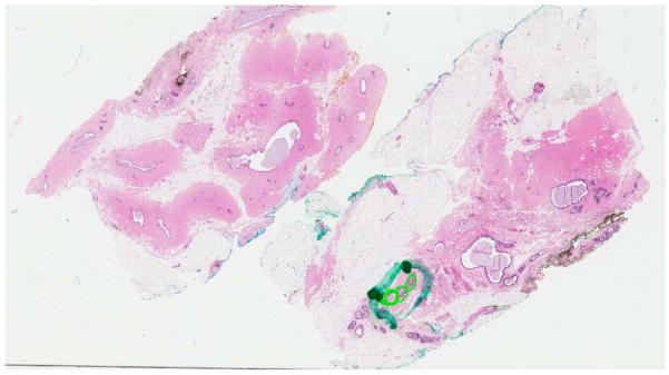
The snapshot of the digitized scan of a H&E stained specimen with three ROIs.
B. Segmentation
H&E stain colors the basophilic structures consisting of nuclear and cytoplasmic regions with blue-purple hue, the protein rich structures consisting of extracellular regions with hues of pink, and red blood cells (RBCs) and regions with necrosis with hues of red. Images of two sample ROIs, one for UDH and the other one for DCIS, are shown in Figures 2a and 2d.
Fig. 2.

The segmentation of the cells for two sample ROIs obtained from a borderline UDH and DCIS cases respectively.
Pathologists use cytological descriptors such as cell size, shape, composition, nuclear spacing etc., evident in the H&E stained tissue specimens for diagnosis. Therefore, cell segmentation would be the first step toward automated analysis of histopathological slides. This is implemented in two steps in this study. In the first step cell regions are segmented by clustering the pixel data and in the second step segmented cell regions are further processed by a watershed-based segmentation algorithm to identify individual cells.
1) Cell region segmentation
The ROI images are first converted from the RGB color space to the La*b* color space. La*b* is a perceptually uniform color space, i.e., a change of the same amount in a color value produces a change of about the same visual importance. The La*b* color space also separates the luminance and the chrominance information such that L channel corresponds to illumination and a* and b* channels correspond to color opponent dimensions.
Pixel data are modeled by a 4-component Gaussian mixture model (GMM). One component is used for each of the following four cytological regions: cellular (nuclear and cytoplasmic), extra-cellular, regions with hues of red and illumina. The expectation maximization (EM) algorithm [6] is implemented using the a*, b* channels to estimate the parameters of the GMM model. The resulting mixture distribution is used to classify pixels into four categories. Those classified into the cellular component are further clustered in the L channel by dynamic thresholding [7] to eliminate blue-purple pixels with relatively less luminance. The remaining pixels are considered cell regions and images containing these regions are used in the next stage.
The EM algorithm is run only once with a dataset containing few million pixels, which are obtained by randomly sampling 10,000 pixels from each ROI image in the dataset. The same GMM model is used for segmenting all ROI images without rerunning EM for each image. Since each slide might contain several ROIs, estimating the distribution offline and using it across all the ROI images saves significant online execution time. Figures 2b and 2e show the segmentation maps of the cell regions in sample ROI images associated with a DCIS and a UDH case respectively.
2) Individual cell segmentation
Segmentation maps of cell regions obtained in the previous part are converted to gray level images before they are used in this stage. Since most segmented regions contain multiple overlapping cells with cells only vaguely defined due to the presence of holes inside them, connected components in these images do not necessarily represent individual cells. These images are first preprocessed using hole filling and cleaning steps suggested in [8]. Overlapped cells result in blobs in the segmentation map. To separate these blobs properly so as to identify individual cells, we used a watershed algorithm based on immersion simulations [9]. In this approach a gray-level image is considered a topographic relief where the gray level of a pixel is interpreted as its elevation. The water flows along a topographic relief following a certain descending path to eventually reach a catchment basin. Blobs in the image can be separated using this concept by identifying the limits of adjacent catchment basins and then separating them. The lines separating catchment basins are called watersheds. The implementation of this algorithm is available through the ImageJ platform [10]. This specific implementation uses the local maxima in the Euclidean distance map as seed points. These seed points are dilated as far as possible either until the edge of the particle or the edge of the region of another growing seed point is reached. We used the Matlab®(Natick, MA) interface to ImageJ to use this implementation alongside our own algorithms. Once all catchment basins are identified and separated with this approach, the region defined by a catchment basin is considered a cell region. These are easily identified in the resulting image by identifying connected components. Figures 2c and 2f show the segmentation maps of the individual cells in sample ROI images associated with a DCIS and a UDH case respectively.
C. Feature Extraction
This section discusses feature extraction methods implemented for quantitative characterization of ROIs in H&E stained slides. Pathologists tend to rely heavily on morphological features such as cell size, shape, and nucleoli apperance. Three different sets of statistical features are computed for each ROI to model these histological descriptors. Perimeter is used for cell size, the ratio of major to minor axis of the best fitting ellipse is used for cell shape, and the mean of the gray level intensity is used for nucleoli apperance. For comparison, summaries of the set of features used by the pathologists for classifying intraductal breast lesions and those employed in the computerized system are reported in Tables I and II, respectively. There are several hundred connected components present in each segmented image. Once the perimeter, the ratio of major to minor axis, and the mean of the gray level intensity are computed for each connected component identified in an ROI, statistical features involving the mean, standard deviation, median, and mode are computed to obtain features at the ROI level. Thus, each ROI is characterized by a total of 12 features (3 × 4).
TABLE I.
Qualitative features used by pathologists for diagnosis.
| Histological Features |
Description |
|---|---|
| Cell Size | Small for UDH, small or medium-sized for ADH and low-grade DCIS, large for high-grade DCIS |
| Cell Shape | Ovoid and mixed for UDH, monotonous for ADH and low-grade DCIS, large and pleomorphic for high-grade DCIS |
| Nucleoli | Indistinct for UDH, single and small for ADH and low-grade DCIS, prominent and enlarged for highgrade DCIS |
TABLE II.
Morphological and pixel intensity features considered in computerized diagnosis.
| Features | Description |
|---|---|
| Perimeter | The perimeter of each connected component is used to characterize cell size. |
| Ratio of major to minor axis |
The ratio of major to minor axis for the best fitting ellipse corresponding to each connected component is used to characterize cell shape (ovoid vs. circular). |
| Mean of the gray level intensity |
The mean of the gray level intensity for each con- nected component is used to characterize nucleoli appearance. Nucleoli, if prominent and/or large, appears darker than cytoplasmic regions in the cell. |
D. Classifier Training
Each slide contains multiple regions of interest and a positive (actionable) diagnosis is confirmed when at least one of the ROIs in the slide is identified as positive. For a negative diagnosis (UDH) the pathologist has to rule out the possibility of each and every ROI being actionable. The objective here is to develop a classifier to optimize classification accuracy at the slide level. Traditional supervised training techniques which are trained to optimize classifier performance at the instance level yield suboptimal performance in this problem.
The problem of learning with multiple instances (MIL) was first defined in the context of a drug activity prediction application [11]. In our earlier work we have developed a MIL approach based on the convex-hull idea and performed experimental studies on two different computer-assisted detection applications which demonstrated that our approach significantly improves detection accuracy when compared to other MIL techniques proposed in the literature [12]. Since this approach was developed for problems where only positive samples are characterized by multiple instances, it was not directly applicable to the histopathological classification problem where negative cases also contain multiple instances. In a more recent work we have proposed an extension of this approach by defining a pair of asymmetric loss functions for positive and negative samples in a large-margin framework and presented results on a dataset containing 40 histopathology slides (20 UDH and 20 DCIS) that showed competitive performance with the state-of-the-art [13].
In what follows, we first provide a brief overview of the large margin principle [14] and then briefly discuss our earlier work on MIL in [13]. The words sample and instance refers to a pathology slide and ROI respectively. As such slide/sample and ROI/instance are used interchangeably throughout this text.
1) Margin maximization with single instance per sample
Notation: When each sample is characterized by a single instance the following notation holds. denotes a training dataset with N samples where is an instance (d-dimensional feature vector) characterizing sample i and is the corresponding known label. In the large margin approach the classifier function f(x) = w · x+w0 is optimized by solving the following optimization problem with respect to w and w0.
| (1) |
where (·)+ = max(0, ·) represents the hinge loss function, and C is the cost preassigned to the misclassification associated with xi.
2) Margin maximization with multiple instances per sample
Notation: In the MIL framework we use the following notation:
| (2) |
where is the feature vector characterizing the jth ROI in slide i, Mi is the number of ROIs in slide i and contains the label information, which is available at the slide level only.
The MIL extension of the problem in (1) can be obtained by defining different loss functions for positive and negative samples such that a positive sample is penalized only when all of its instances, i.e., all ROIs in that slide, are classified negative, whereas a negative sample is penalized when at least one of its instances is classified positive. Next, we define two new loss functions for positive and negative samples.
Loss function for negative samples
For negative cases loss is incurred when at least one of the ROIs in a slide is classified as positive. Thus, we replace the hinge loss function used in (1) with its multivariable counterpart defined by
| (3) |
where . This ensures that the loss incurred by a negative slide i is zero only if all ROIs in the slide are correctly classified as negative.
Loss function for positive cases
For positive cases loss is incurred when all of the ROIs in a slide are classified as negative. In other words for correct diagnosis, it is sufficient to identify at least one ROI on a slide as positive. If a point that lies within the convex hull of all the instances of a sample is classified positive, this will indicate that at least one of the original ROIs is also classified positive. Let λi s.t. , e · λi = 1 be the vector containing the coefficients of the convex combination of all ROIs in slide i, and e be a vector of ones. Then the feature vector characterizing slide i is defined by
| (4) |
where is the data matrix containing feature vectors of all ROIs within slide i. The loss function for a positive case in this new framework can be defined by
| (5) |
which is a function of both convex-hull coefficients λi and classifier coefficients w. More detailed discussion on convexhull characterization of samples with multiple instances can be found in our earlier work in [12]. With the new loss functions for positive and negative samples added to the problem, the large-margin formulation becomes:
| (6) |
where Ω+ and Ω− are the corresponding sets of indices for the positive and negative samples respectively, and the two constraints are imposed to ensure that the feature vector characterizing a positive sample is always within the convexhull of its instances. This problem can be optimized by iterating between two convex subproblems in an alternating manner. The first subproblem optimizes for w and w0, while λi are fixed. The second subproblem optimizes for λi while w and w0 are fixed. Since both subproblems are convex the objective function in (6) is guaranteed to decrease after each iteration. Thus, convergence can be established by defining a termination criteria, based on the change in the value of the objective function between any two iterations.
III. Results
In this section experiments are performed to validate the stand-alone performance of the developed system. To avoid numerical problems during optimization it is a common preprocessing step to normalize each feature to between -1 and 1. The parameters of the classifiers are selected from a designated set of six different C+ and C− values by considering all possible pairs (6 × 6 = 36 pairs) and selecting the pair that optimizes the leave-one-slide-out (LOSO) cross validation performance of the classifier. LOSO cross-validation splits the training dataset into k folds, where k is equivalent to the number of slides. At each stage one slide is left out as validation data, i.e., all ROIs for that slide are removed from the training data as validation data, and the classifier is trained with the ROIs of the remaining k – 1 slides and tested on the ROIs of the left-out slide. This process is repeated until all k slides are used for validation and the probabilities of all ROIs being positive are obtained. There is only one slide for eachpatient in our study database. Thus, each fold only contains data from a unique patient. In this regard, the LOSO approach used in this study is the same as leave-one-patient-out (LOPO) cross validation. The classifier performance is measured by the area under the receiver operating characteristic (ROC) curve, or the so called Az value. The different operating points along the ROC curve are obtained by comparing the classification results with the reference standard available for each case at varying thresholds, θ, i.e., f(x) >= θ. Once the pair of classifier parameters that maximizes the Az value is determined the classifier is trained with the entire training dataset to obtain the classifier function f(x) = w · x + w0. The two features with the largest weights in the optimized weight vector, w, are the mean of the mean intensity and the median of the ratio of the major to minor axis of the best fitting elipse. The first one characterizes nucleoli prominence and the second one cell shape.
Figure 3a shows the ROC curve obtained by LOSO on the training data along with the ROC curve obtained on the test data. Az values of 0.92 and 0.93 are achieved respectively on the training and test datasets.
Fig. 3.

(a) ROC curves obtained for the training (62 cases by LOSO) and test sets (33 cases) using the proposed approach (MILSVM). (b) ROC curves comparing MILSVM with other techniques from the literature on the test set.
Next, the classifier defined by the classification boundary, f(x) = 0, is evaluated for each ROI on the test data. ROIs with f(x) > = 0 are classified positive, whereas those with f(x) < 0 are classified negative. Here x respresents the feature vector characterizing the ROI. Classification at the slide level is rendered by classifying slides with at least one positive ROI as actionable and those where all ROIs are negative as UDH. An overall accuracy of 87.9% (29/33) is achieved by the computerized system. We also compared the accuracy of the system against the accuracies of the nine pathologists. These are the same group of nine pathologists used to establish the reference standard for each case in the study database. However this step is different than truthing in that pathologists were provided immunostained serial sections of the specimens so that an accurate reference standard could be obtained for each case. This time pathologists are only provided H&E stained serial sections for evaluation and are instructed to classify each case as UDH, ADH, and DCIS. Cases classified ADH or DCIS by the pathologists are grouped together under the actionable category. The study with the pathologists is performed using only the borderline cases in the test set (26 out of 33). The classification accuracies of the nine pathologists are presented in Table III.
TABLE III.
Classification accuracies (%) of the nine pathologists on borderline cases.
| 1 | 2 | 3 | 4 | 5 | 6 | 7 | 8 | 9 | Avg. | |
|---|---|---|---|---|---|---|---|---|---|---|
| Pathologists: | 84.6 | 84.6 | 57.7 | 84.6 | 92.3 | 77.0 | 96.2 | 77.0 | 77.0 | 81.2 |
We believe that the accuracy of 87.9% achieved on all test cases and of 84.6% achieved on borderline cases by the computerized system is quite promising. The accuracy on borderline cases is better than the accuracy of the four pathologists and is in par with the accuracy achieved by three of the remaining five pathologists. When we take a closer look at the four cases misclassified by the computerized system, we see that three of them are UDH and one is actionable. However, these are cases for which pathologists did not have complete agreement either. One case is classified UDH by five pathologists and actionable by the remaining four. The other case is classified actionable by six pathologists and UDH by the remaining three. The other two cases are classified actionable by seven pathologists and UDH by the remaining two.
Finally, we compared the performance of the proposed MIL approach (MILSVM) with two other MIL techniques from the literature, namely the MIL versions of the relevance vector machine (MILRVM) [15] and AND-OR SVM [16]. Two traditional supervised training techniques, namely RVM [17] and linear SVM [14] are also included in this comparative analysis. All classifiers are tuned by LOSO using the training set and are validated with the test set. The receiver operating characteristics (ROC) curves obtained for the five classifiers are shown in Figure 3b along with the Az values achieved by each. The proposed approach achieves an Az value of 0.93. The second largest Az=0.87 is achieved by SVM. Significance analysis between the two ROC curves using the approach in [18] yields a p-value of 0.048, which indicates the improvement is statistically significant.
IV. Conclusions
In this study a system for computerized analysis of breast microscopic tissues is developed for improved classification of intraductal breast lesions. The system is developed with 62 cases and tested on 33 cases. An overall accuracy of 87.9% is achieved on the entire test set involving 7 welldefined and 26 borderline cases. An accuracy of 84.6% is recorded on borderline cases. This was slightly higher than the average accuracy of nine board-certified pathologists (81.2%) evaluated on the same set. We believe that the stand-alone classification performance of the developed system is highly encouraging. However, before this system can be deployed in a clinical setting as a “second reader” its incremental value has to be assessed. Before such a study can be effectively carried out, the computerized system has to be improved such that its output is presented in a way that could easily be interpreted by the pathologists. This will involve developing intermediate models to map image features onto descriptors pathologists use for classification. Apart from making the output of the system more interpretable, we will also increase the size of the study database for more extensive testing of the developed system. Once these two goals are achieved, a reader study involving a panel of pathologists with varying levels of experience will be conducted to evaluate the incremental value of the computerized system as a second reader.
ACKNOWLEDGMENT
The project described was supported in part by Award Number R01CA134451 from the National Cancer Institute. The content is solely the responsibility of the authors and does not necessarily represent the official views of the National Cancer Institute, or the National Institutes of Health.
Biography

Dr. M. Murat Dundar (M’06) is currently an Assistant Professor in the Department of Computer and Information Science at IUPUI. He received his BS degree from Bogazici University, Istanbul, Turkey, in 1997 and his MS and PhD degrees from Purdue University, West Lafayette, IN, USA, in 1999 and 2003 respectively, all in Electrical Engineering. His research interests include machine learning with applications to computer aided diagnosis, medical image mining, biosensing, and remote sensing.

Dr. Sunil Badve is a Professor in the department of Pathology and Laboratory Medicine, with an additional appointment in department of Internal Medicine at Indiana University. He received his MD degree from Bombay University, Bombay, India, in 1986, completed his residency at the Albert Einstein College of Medicine, Bronx, NY, in 1998, and his fellowship at Yale University School of Medicine, New Haven, CT, 1999. He serves as the Director of Translational Genomics Core at the Indiana University Cancer Center. Dr. Badve’s main research and clinical expertise is in breast cancer. He is the breast Pathologist for Eastern Co-operative Oncology group, where he serves as the Pathology Chair for several breast cancer clinical trials including the TAILORx clinical trial based on the Oncotype Dx assay.

Dr. Gokhan Bilgin is currently a postdoctoral researcher in the Department of Computer and Information Science at IUPUI. He received his BS, MS, and PhD degrees from Yildiz Technical University, Istanbul/Turkey, all in the Electronics and Telecommunications department. His research interests are in the areas of image and signal processing and machine learning with applications to biomedical engineering and remote sensing.

Dr. Vikas Raykar currently works as a scientist in the CAD R&D division for Siemens Healthcare, USA. He received his BS degree from the National Institute of Technology, Trichy, India, MS and PhD degrees from the University of Maryland, College Park, MD, USA. His research interest is in the area of machine learning with an emphasis on fast computational methods.

Rohit Jain received his Bachelor of Medicine and Bachelor of Surgery (MBBS) degree from Topiwala National Medical College, India and his Masters degree in Public Health (MPH) from Indiana University, Indianapolis in May 2010. He is currently assisting Dr. Sunil Badve, a breast cancer pathologists on several of his research projects. His research interests lie mainly in the field of translational cancer research.

Dr. Olcay Sertel is currently working as an Image Analysis Scientist at Ventana Medical Systems, a member of Roche group. He received his Ph.D. degree in Electrical and Computer Engineering from The Ohio State University in 2010. He worked as a Research Associate at the Dept. of Biomedical Informatics, The Ohio State University during 2006-2010. He received his M.Sc. degree from Yeditepe University, Istanbul, Turkey in 2006 and B.Sc. degree from Yildiz Technical University, Istanbul, Turkey in 2004 both in computer engineering. His research interests include image processing and analysis, computer vision and statistical pattern recognition with applications in medicine.

Dr. Metin N. Gurcan is an Associate Professor of Biomedical Informatics at the Ohio State University. He received his BSc. and Ph.D. degrees in Electrical and Electronics Engineering from Bilkent University, Turkey and his MSc. Degree in Digital Systems Engineering from the University of Manchester Institute of Science and Technology, England. He is the recipient of the British Foreign and Commonwealth Organization Award, Children’s Neuroblastoma Cancer Foundation Young Investigator Award and National Cancer Institute’s caBIG Embodying the Vision Award. Dr. Gurcan’s research interests include image analysis and understanding, computer vision with applications to medicine. Dr. Gurcan is a senior member of IEEE since 2006. He is also a senior member of SPIE and RSNA.
Contributor Information
M. Murat Dundar, Department of Computer & Information Science, Indiana University - Purdue University, Indianapolis, IN 46202 USA dundar@cs.iupui.edu.
Sunil Badve, Department of Pathology, Indiana University, Indianapolis, IN 46202 USA.
Gokhan Bilgin, Department of Computer & Information Science, Indiana University - Purdue University, Indianapolis, IN 46202 USA gbilgin@cs.iupui.edu.
Vikas Raykar, Siemens Healthcare, Malvern, PA 19355 USA vikas.raykar@siemens.com.
Rohit Jain, Department of Pathology, Indiana University, Indianapolis, IN 46202 USA.
Olcay Sertel, Biomedical Informatics Department, The Ohio State University, Columbus, OH 43210 USA.
Metin N. Gurcan, Biomedical Informatics Department, The Ohio State University, Columbus, OH 43210 USA.
REFERENCES
- [1].Tavassoli FA, Devilee P. World Health Organization: Tumours of the Breast and Female Genital Organs (IARC WHO Classification of Tumours) IARCPress-WHO; 2003. [Google Scholar]
- [2].Fitzgibbons PL, Page DL, Weaver D, Thor AD, Allred DC, Clark GM, Ruby SG, O’Malley F, Simpson JF, Connolly JL, Hayes DF, Edge SB, Lichter A, Schnitt SJ. Prognostic factors in breast cancer. Archives of Pathology & Laboratory Medicine. 2000;vol. 124(7):966–978. doi: 10.5858/2000-124-0966-PFIBC. [DOI] [PubMed] [Google Scholar]
- [3].Rozai J. Borderline epithelial lesions of the breast. Am J Surg Pathol. 1991;vol. 15(3):209–21. doi: 10.1097/00000478-199103000-00001. [DOI] [PubMed] [Google Scholar]
- [4].Jain R, Mehta R, Dmitrov R, Larsson L, Musto P, Hodges K, Ulbright T, Hattab E, Agaram N, Idrees M, Badve S. Atypical ductal hyperplasia at 25 yearsinterobserver and intraobserver variability. Mod Pathol. 2010;vol. 23(1):53A. doi: 10.1038/modpathol.2011.66. supp no.1. abstr 229. [DOI] [PubMed] [Google Scholar]
- [5].Page D, Dupont W, Rogers L, Rados M. Borderline epithelial lesions of the breast. Am J Surg Pathol. 1991;vol. 15:209–221. doi: 10.1097/00000478-199103000-00001. [DOI] [PubMed] [Google Scholar]
- [6].Dempster AP, Laird NM, Rubin DB. Maximum likelihood from incomplete data via the em algorithm. (Series B (Methodological)).Journal of the Royal Statistical Society. 1977;vol. 39(no. 1):1–38. [Online]. Available: http://dx.doi.org/10.2307/2984875. [Google Scholar]
- [7].Otsu N. A threshold selection method from gray-level histograms. IEEE Transactions on Systems, Man, and Cybernetics. 1979;vol. 9(1):62–66. [Google Scholar]
- [8].Eddins S. Cell segmentation. 2006 [Online]. Available: http://blogs.mathworks.com/steve/2006/06/02/cell-segmentation/
- [9].Vincent L, Soille P. Watersheds in digital spaces: An efficient algorithm based on immersion simulations. IEEE Pattern Analysis and Machine Intelligence. 1991;vol. 13(6):583–98. [Google Scholar]
- [10].Rasband W. Imagej. U. S. National Institutes of Health; Bethesda, Maryland: 1997-2009. http://rsb.info.nih.gov/ij/ [Online]. Available: http://rsb.info.nih.gov/ij/ [Google Scholar]
- [11].Dietterich TG, Lathrop RH, Perez T. Lozano. Solving the multiple-instance problem with axis-parallel rectangles. Artificial Intelligence. 1997;vol. 89(no. 1-2):31–71. [Google Scholar]
- [12].Fung G, Dundar M, Krishnapuram B, Rao RB. Multiple instance learning for computer aided diagnosis. In: Schölkopf B, Platt J, Hoffman T, editors. Advances in Neural Information Processing Systems 19. MIT Press; Cambridge, MA: 2007. pp. 425–432. [Google Scholar]
- [13].Dundar MM, Badve S, Raykar V, Jain RK, Sertel O, Gurcan MN. A multiple instance learning approach toward optimal classification of pathology slides: A case study: Intraductal breast lesions. Proceedings of the 20th International Conference on Pattern Recognition, August 23-26; Istanbul, Turkey. 2010. pp. 2732–2735. [Google Scholar]
- [14].Vapnik VN. The Nature of Statistical Learning Theory. Springer; New York: 1995. [Google Scholar]
- [15].Raykar VC, Krishnapuram B, Bi J, Dundar M, Rao RB. Bayesian multiple instance learning: automatic feature selection and inductive transfer. ICML ’08: Proceedings of the 25th international conference on Machine learning; New York, NY, USA. ACM; 2008. pp. 808–815. [Google Scholar]
- [16].Wu D, Bi J, Boyer K. A min-max framework of cascaded classifier with multiple instance learning for computer aided diagnosis. 2009 IEEE Computer Society Conference on Computer Vision and Pattern Recognition (CVPR 2009); Miami, FL, USA. 20-25 June 2009. [Google Scholar]
- [17].Tipping ME. The relevance vector machine. In: Solla S, Leen T, Muller K-R, editors. Advances in Neural Information Processing Systems 12. MIT Press; Cambridge, MA: 2000. pp. 652–658. [Google Scholar]
- [18].Hanley JA, McNeil BJ. A method of comparing the areas under receiver operating characteristic curves derived from the same cases. Radiology. 1983;vol. 148:839–843. doi: 10.1148/radiology.148.3.6878708. [DOI] [PubMed] [Google Scholar]