Network Analysis of Corticocortical Connections Reveals Ventral and Dorsal Processing Streams in Mouse Visual Cortex

Abstract

Much of the information used for visual perception and visually guided actions is processed in complex networks of connections within the cortex. To understand how this works in the normal brain and to determine the impact of disease, mice are promising models. In primate visual cortex, information is processed in a dorsal stream specialized for visuospatial processing and guided action and a ventral stream for object recognition. Here, we traced the outputs of 10 visual areas and used quantitative graph analytic tools of modern network science to determine, from the projection strengths in 39 cortical targets, the community structure of the network. We found a high density of the cortical graph that exceeded that shown previously in monkey. Each source area showed a unique distribution of projection weights across its targets (i.e., connectivity profile) that was well fit by a lognormal function. Importantly, the community structure was strongly dependent on the location of the source area: outputs from medial/anterior extrastriate areas were more strongly linked to parietal, motor, and limbic cortices, whereas lateral extrastriate areas were preferentially connected to temporal and parahippocampal cortices. These two subnetworks resemble dorsal and ventral cortical streams in primates, demonstrating that the basic layout of cortical networks is conserved across species.

Introduction

The discovery that outputs from primate primary visual cortex (V1) flow through distinct dorsal and ventral streams (Ungerleider and Mishkin, 1982; Goodale and Milner, 1992) has raised the question whether similar pathways exist in the visual system of afoveal rodents (Livingstone and Hubel, 1988; McNaughton et al., 1989; Salinas-Navarro et al., 2009). Although the scheme received support from behavioral observations in rat (Kolb, 1990), cortical streams have not been demonstrated anatomically.

Studies in primates have shown that the ventral stream uses visual information for object recognition, whereas the dorsal stream is specialized for spatial perception and visually guided actions (Kravitz et al., 2011). In rodents, the notion of “two visual systems ” originated from studies in hamster, which showed that the cortex plays a role in recognizing “what ” an object is, whereas taking action “where ” to move was thought to be determined by the optic tectum (Schneider, 1969). This explanation was later revised by experiments in rats, which showed that lesions in the temporal cortex interfere with object recognition, whereas lesions in the parietal cortex impair spatial orientation (Kolb et al., 1994; Tees, 1999; Ho et al., 2011). Based on these findings, it was proposed that rodents have functionally specialized cortical streams. Indeed, it seems plausible that evolution has selected separate systems for recognizing predators and for navigating routes of escape (Livingstone and Hubel, 1988). Support for this organization comes from studies in rat that show that inputs to the amygdala, a nucleus involved in the acquisition and expression of fear, derive from ventral but not from dorsal extrastriate visual cortex (McDonald and Mascagni, 1996).

Mouse visual cortex contains ≥10 areas (Wang and Burkhalter, 2007), whose topographic organization was recently confirmed by calcium imaging of visual responses (Marshel et al., 2011). Many of these areas receive inputs from the thalamus, but the most direct and strongest visual input to V1 derives from parallel retino-geniculate pathways (Frost and Caviness, 1980; Simmons et al., 1982) specialized for high spatial/low temporal and low spatial/high temporal sensitivity (Gao et al., 2010). Outputs from V1 are distributed across many cortical regions, among these to at least nine extrastriate visual areas (Olavarria and Montero, 1989; Wang and Burkhalter, 2007). The strongest of these outputs terminate in the lateromedial (LM) and anterolateral (AL) extrastriate visual areas on the lateral side of V1. Outputs from LM are biased to ventral regions, whereas AL projects more strongly to dorsal cortex, suggesting that these areas are gateways of ventral and dorsal streams (Wang et al., 2011). To determine the nodes of these streams, we traced the connections of 10 areas of mouse visual cortex. Quantitative assessments of connection strengths, cluster, and graph analyses demonstrate that visual areas are segregated into interconnected dorsal and ventral modules that are reminiscent of dorsal and ventral streams in primates.

Materials and Methods

Experiments were performed in 6- to 8-week-old C57BL/6J male and female mice. All experimental procedures were approved by the Institutional Animal Care and Use Committee at Washington University and conformed to the National Institutes of Health guidelines.

Tracer injections.

For tracer injections, male and female mice were anesthetized with a mixture of ketamine (86 mg/kg) and xylazine (13 mg/kg, i.p) and secured in a head holder. The body temperature was maintained at 37°C. In each animal, the callosal and the ipsilateral cortical connections were labeled on the left side of the brain. Callosal connections were retrogradely labeled by making 30–40 pressure injections (Picospritzer; Parker-Hannafin) with glass pipettes (20 μm tip diameter) of bisbenzimide (5% in H₂O, 20 nl each; Sigma) into the right occipital, temporal, and parietal cortices. Local intracortical connections within the left hemisphere were anterogradely labeled by inserting glass pipettes (15 μm tip diameter) into the brain and iontophoretic injection (3 μA, 7 s on/off duty cycle for 7 min; Midgrad current source; Stoelting) of biotinylated dextran amine (BDA; 10,000 molecular weight, 5% in H₂O, 20 nl; Invitrogen). Injections were performed stereotaxically 0.35 mm below the pial surface, using a coordinate system whose origin was the intersection between the midline and a perpendicular beam drawn from the anterior border of the transverse sinus at the pole of the occipital cortex. The coordinates of the injected areas were (anterior/lateral in mm): V1, 1.1/2.8; LM, 1.4/4.1; AL, 2.4/3.7; posterior (P), 1.0/4.2; laterointermediate (LI), 1.45/4.2; postrhinal (POR), 1.15/4.3; rostrolateral (RL), 2.8/3.3; anterior (A), 3.4/2.4; posteromedial (PM), 1.9/1.6; anteromedial (AM), 3.0/1.7.

Histology.

Three days after the tracer injections, mice were deeply anesthetized with an overdose of ketamine/xylazine and perfused through the heart with PBS, followed by 1% paraformaldehyde (PFA) in 0.1 m phosphate buffer, pH 7.4. The cortex was immediately separated from the rest of the brain, flattened or completely unfolded, placed white matter down on a filter paper laying on top of a thin strip of sponge, and covered with a glass slide (25 × 75 × 1 mm). The assembly was postfixed in a Petri dish filled with 4% PFA and stored overnight at 4°C. After postfixation, the tissue was cryoprotected in 30% sucrose and cut on a cryostat or freezing microtome in the tangential plane at 50 μm.

To identify the injected area as well as the targets of anterogradely BDA-labeled projections, we visualized in every case the regional myeloarchitecture and the callosal connections. Previously, we have used these landmarks as reference to locate and/or directly identify the visuotopically organized areas V1, LM, P, LI, POR, AL, RL, A, PM, and AM (Wang and Burkhalter, 2007). Both histological patterns were imaged in wet-mounted sections with a CCD camera (CoolSnap EZ; Photometrics). Sections through layer 4 were imaged under a dissecting microscope (Wild M5, Leica), equipped with dark-field optics. Under these conditions, heavily myelinated areas appeared lighter than the background (Fig. 1c). Sections through layer 2/3 were imaged under a fluorescence microscope (Nikon Eclipse 80i) equipped with UV optics. This illumination revealed blue retrogradely bisbenzimide-labeled callosal projection neurons (Fig. 1a). To parcel the rest of cortex in which myeloarchitecture and callosal patterns showed less structure, we stained complete sets of sections of each BDA-injected hemisphere with an antibody against type 2 muscarinic acetylcholine receptor (m2AChR; MAB367; Millipore), visualized the expression with Alexa Fluor 647-labeled secondary antibody (A21247; Invitrogen) and imaged the sections under infrared fluorescence (Wang et al., 2011). To further validate the m2AChR-based parcellation scheme, we stained alternate series of tangential sections from three flat-mounted hemispheres, which were not injected with BDA, for cytochrome oxidase (CO) histochemistry and Nissl substance. BDA-labeled projections were visualized by incubating sections in avidin and biotinylated HRP (Vectastain ABC Elite) and intensifying the diaminobenzidine reaction product with AgNO₃ and HAuCl₂ (Jiang et al., 1993). The reacted sections were dehydrated, cleared, and coverslipped with DPX. The intensified, BDA-labeled sections were imaged under dark-field illumination.

Figure 1.

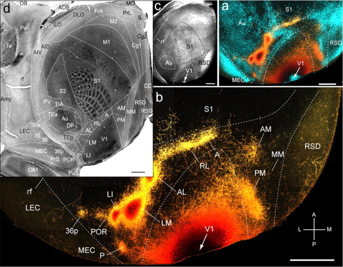
Connections of V1 in tangential sections through flat-mounted mouse cerebral cortex. a, b, Dark-field image of anterogradely labeled axonal projections (yellow, high-density clusters are marked by even higher-density red–brown centers) after injection of BDA into V1 (arrow). Blue labeling in a represents landmark pattern of retrogradely bisbenzimide-labeled callosal projection neurons. c, Dark-field image of wet-mounted, unstained section through layer 4, showing bright myelin-rich cortical fields. d, CO-stained tangential section through layer 4, showing differential expression across cerebral cortex. Scale bars, 1 mm. Axes: A, anterior; P, posterior; M, medial; L, lateral. Arrows indicate injection site. A, Anterior; AID, anterior dorsal insula; AIV, anterior ventral insula; AL, anterolateral; AM, anteromedial; Amy, amygdala; AOB, accessory olfactory bulb; Au, auditory; CA1, hippocampus; CC, corpus callosum; Cg1, cingulate 1; Cg2, cingulate 2; DA, dorsal anterior; DLO, dorsal lateral orbital; DP, dorsal posterior; FrA, frontal association; IL, infralimbic; LEC, lateral entorhinal; LI, lateral intermediate; LM, lateral medial; LO, lateral orbital; M1, motor 1; M2, motor 2; MEC, medial entorhinal; MM, mediomedial; MO, medial orbital; OB, olfactory bulb; P, posterior; PaS, parasubiculum; Pir, piriform; PM, posterior medial; POR, postrhinal; PrL, prelimbic; PrS, presubiculum; PV, parietal ventral; rf, rhinal fissure; RL, rostrolateral; RSD, retrosplenial dysgranular; RSG, retrosplenial granular; S1, somatosensory 1; S2, somatosensory 2; TEa, temporal anterior; TEp, temporal posterior; Tu, olfactory tubercle; V1, primary visual; VO, ventral orbital. Abbreviations apply to subsequent figures.

Digital overlays of BDA-labeled projections with images of the myeloarchitecture, callosal connections, m2AChR, and CO staining patterns were used for assigning terminal clusters to cortical areas. Superimpositions with m2AChR immunofluorescence were performed by matching blood vessels within the same case. Alignments with CO patterns were done across cases, by first overlying the intensely labeled areas V1 and primary somatosensory cortex (S1) with corresponding myeloarchitectonic regions of another brain and then matching the BDA-labeled projections to the CO-stained template.

Optical densitometry.

The strength of BDA-labeled projections was determined by optical densitometry (Wang et al., 2011). Densitometric measurements were made in bright-field images taken with a CCD camera at 4×. The images were then analyzed with customized Matlab software. Projections were identified as clusters of terminal axon branches with high bouton density. The optical density of each projection was determined at four different depths of the superficial 400 μm of cortex. Deep layers were excluded to minimize potential contamination of optical density measurements by fibers of passage, which in rodents often travel through layers 5 and 6 (Coogan and Burkhalter, 1993). Optical densities were determined relative to the darkest region at the center of the injection site and scaled to the unstained background. Blood vessels were subtracted from the image as white unstained profiles, and a 5 μm Gaussian blur was applied. The absolute density of a projection represented the average across the four levels of cortical gray matter. The strength of a given projection was expressed as percentage of the sum total of projection densities across all areas of cortex labeled by a single injection. Mean ± SEM relative density measurements from three to four mice were averaged and plotted for each projection target. We have shown previously that optical density is tightly correlated with bouton density (Wang et al., 2011) and therefore likely reflects the strength of synaptic connections.

Retrograde labeling.

BDA mostly anterogradely labeled axons and axon terminals. However, in some cases, BDA also retrogradely labeled small numbers of neurons. Although retrograde labeling was much too sparse to significantly affect the density of anterograde labeling, it was consistent enough to assess qualitatively whether reciprocal connections were present.

Network analyses.

For quantitative network analysis, the mean estimates for the strengths of projections obtained by optical densitometry were combined into a 10 × 40 connection matrix (10 source regions, 39 target regions, plus self-connections that are set to zero). A smaller 10 × 10 submatrix M consisted of all interconnections between the 10 source regions, including all reciprocal projections. In addition to connection densities, we estimated projection lengths between the 10 source regions by using a standard flat map of cortex (Fig. 1d) and measuring the Euclidian distances between the center-of-mass coordinates of different brain regions, determined with customized Matlab software.

We used several standard clustering and dimension reduction techniques, including k-means, nonmetric multidimensional scaling (NMDS), and principal component analysis (PCA), to assess the similarity of projection profiles. Treating the anatomical data as a network of areas and inter-areal projections (nodes and edges), we applied several graph-theoretical measures, available as part of the Brain Connectivity Toolbox (Rubinov and Sporns, 2010) to the fully weighted M submatrix. These measures were chosen to gain additional insights into the community structure of the visual network. We computed the modularity and the optimal modularity partition of M using a modularity metric that is based on the density of connections within modules relative to the density between modules (Girvan and Newman, 2002). We also derived the matrix of shortest directed paths between all pairs of nodes as well as the nodal betweenness centrality, a measure that captures how many of the shortest paths across the network pass through a given node (Sporns, 2011).

Graph measures were computed on the nearly full matrix M as well as on a reduced matrix M′, identical to M but with the weaker half of all projections removed. This reduced matrix retained 76% of the original projection density. To assess the degree to which graph measures were attributable to the global connection topology and not to connection densities, node degrees, or strengths, we compared graph metrics obtained from the two empirical networks M and M′ to two different random models, respectively. Network M was randomized by randomly reordering incoming projections for each node, thus preserving the total strength of the afferent projections each node. Network M′ was randomized by rewiring projections according to a Markov switching algorithm (Maslov and Sneppen, 2002), thus preserving the in- and out-degree and out-strength of each node. Both random models degraded global connection topology, and all statistical comparisons were performed against samples of 10,000 random networks.

Results

Output of V1

We found that the heavily myelinated area V1 projects to 25 cortical targets (Fig. 1b) (see Fig. 4a). In 19 of them, the projections were strong enough for quantification by scaling their optical density to the summed density of all 19 projections.

Figure 4.

Relative strength of connections labeled after injection of BDA into areas V1, LM, LI, P, POR, AL, PM, RL, AM, and A of mouse visual cortex. a–k, Average ± SEM optical density (y-axis) of a specific projection target (x-axis) scaled by the summed density of all projections labeled by an injection of a specific area (red bar). Target regions indicated in black have unidirectional connections with the source region. Green labels indicate reciprocal connections. Open bars indicate that labeling was not strong enough for quantification. The percentages indicated by arrows represent the strengths of connections (excluding V1) in the ventral (red shading) and dorsal (blue shading) areas.

The strongest projections were highly topographic and terminated in well-defined areas LM, LI, P, POR, posterior area 36 (36p), AL, RL, AM, and PM (Wang and Burkhalter, 2007) contained within the cytoarchitectonic regions designated in the atlas by Franklin and Paxinos (2007) as lateral and medial secondary visual (V2L, V2ML, V2MM), posterior parietal (lateral, medial) association (LPtA, MPtA) areas, and ectorhinal cortex. Injections into the upper field periphery of V1-labeled areas LM, AL, and LI at primarily separate locations within the large acallosal ring in V2L lateral to V1 (Fig. 1a,b). In contrast, lower-field injections labeled a single patch at the shared border between LM, AL, and LI (data not shown) (Wang and Burkhalter, 2007, their Figs. 4B, 5B, 6A). Additional topographic maps were found in the temporal area P, contained within V2L. Ectorhinal cortex (Franklin and Paxinos, 2007) contained visuotopic maps in the parahippocampal areas POR and 36p. Anterior V2L, LPtA, and MPtA (Franklin and Paxinos, 2007) contained maps in the posterior parietal areas RL, A, and AM (Wang and Burkhalter, 2007). Projections to the medial extrastriate cytoarchitectonic field V2ML (Franklin and Paxinos, 2007) terminated in the topographically organized area PM (Wang and Burkhalter, 2007).

Figure 5.

Connections of the LI in tangential sections through flat-mounted mouse cerebral cortex. a, Dark-field image of wet-mounted, unstained section through layer 4 showing bright myelin-rich cortical fields. b, Dark-field image of anterogradely labeled axonal projections (white) after injection of BDA into area LI (arrow). c, Blue labeling represents landmark pattern of retrogradely bisbenzimide-labeled callosal projection neurons. d, Overlay of callosal connections (blue) and BDA-labeled projections (white). Scale bars, 1 mm. Arrows indicate injection site.

Figure 6.

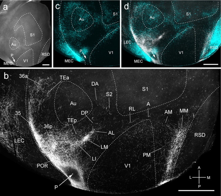
Connections of P in tangential sections through flat-mounted mouse cerebral cortex. a, Dark-field image of wet-mounted, unstained section through layer 4 showing bright myelin-rich cortical fields. b, Dark-field image of anterogradely labeled axonal projections (white) after injection of BDA into area P (arrow). c, Blue labeling represents landmark pattern in of retrogradely bisbenzimide-labeled callosal projection neurons. d, Overlay of callosal connections (blue) and BDA-labeled projections (white). Scale bars, 1 mm. Arrows indicate injection site.

Much sparser projections were found in the septa of S1, the dysgranular (RSD) and granular (RSG) retrosplenial areas (Franklin and Paxinos, 2007), the mediomedial area (MM) (Wang and Burkhalter, 2007) contained within V2MM (Franklin and Paxinos, 2007), the primary cingulate area (Cg1) (Franklin and Paxinos, 2007) located at the crest of the medial wall, and the ventral orbitofrontal area VO (Franklin and Paxinos, 2007) (Fig. 1b) (see Fig. 4a). In addition, sparse inputs were found in lateral and medial entorhinal cortices (MEC, LEC) (Franklin and Paxinos, 2007) as well as the presubiculum (PrS) (Franklin and Paxinos, 2007) (see Fig. 4a). Each of these targets overlapped with previously identified cytoarchitectonic areas (Franklin and Paxinos, 2007) but were distinguished here by CO (Fig. 1d) and m2AChR (Wang et al., 2011) (data not shown) expression. Although this parcellation scheme may be coarser than its cytoarchitectonic counterpart (Franklin and Paxinos, 2007), it is much more discriminating in horizontal sections.

Previously, we have shown that LM projects more strongly to temporal cortex, whereas the outputs of AL favor dorsal and medial cortices (Wang et al., 2011). Here, we show that these projections funnel into mutually interconnected ventral and dorsal streams with multiple nodes. This organization is best illustrated by first showing the projections of areas POR and A, which are far downstream the ventral and dorsal streams, respectively.

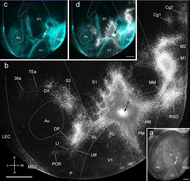
Outputs of POR

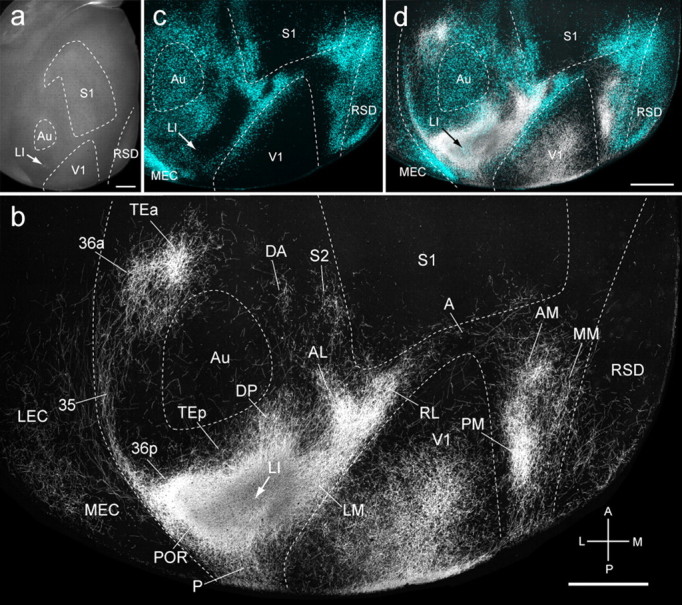
Injections into POR (n = 3) were found in callosally connected parahippocampal cortex bordered by LM, LI, P, and the rhinal sulcus (Fig. 2a,c,d). Projections were observed in 35 cortical targets and were generally stronger in ventral than dorsal cortex (Fig. 2b). Of the total weight of POR projections, 83% terminated in temporal, parahippocampal, and piriform areas, whereas 13% were found in parietal, medial, retrosplenial, cingulate, prefrontal, and orbitofrontal cortices (see Fig. 4e). Within V1, labeling was densest at the lateral border, indicating that the projections originated from the upper nasal representation of POR. In areas LM, AL, and LI, the connections were clustered at distinct locations within the large acallosal ring lateral of V1 (Fig. 2b,d). The projections to the CO-dense areas P and 36p (Fig. 1d) were extremely strong, such that, under dark-field illumination, light scatter was reduced, and weaker inputs to the CO-pale areas 36, 36a, and TEa (anterior temporal) (Fig. 1d), contained within temporal association and secondary ventral auditory cortex (AuV) (Franklin and Paxinos, 2007), appeared paradoxically stronger (Fig. 2b). Strong inputs were found in the CO-pale auditory belt area TEp (posterior temporal) within AuV (Franklin and Paxinos, 2007), whereas inputs to the CO-dense auditory areas Au (primary auditory) and DP (dorsal posterior) within the dorsal auditory belt AuD (Franklin and Paxinos, 2007) were weaker (Figs. 1d, 2b). The projections to the CO/m2AChR-dense (Wang et al., 2011) MEC and more weakly CO-expressing LEC were approximately equally strong (Fig. 2b) (see Fig. 4e). In contrast to the inputs to temporal cortex, projections to dorsal and medial cortices were weak. This includes inputs to the densely CO/m2AChR-expressing areas S1 and RSG, the paler areas of secondary somatosensory (S2) (Wang et al., 2011), posterior parietal (RL, A, AM), posterior medial (PM), Cg1, and the CO-pale MM cortex (Figs. 1d, 2b) (see Fig. 4e). Similarly, weak inputs were found in the CO-pale prefrontal prelimbic (PrL) and infralimbic (IL) (Franklin and Paxinos, 2007) areas as well as the CO-dense VO (Fig. 1d) (see Fig. 4e).

Figure 2.

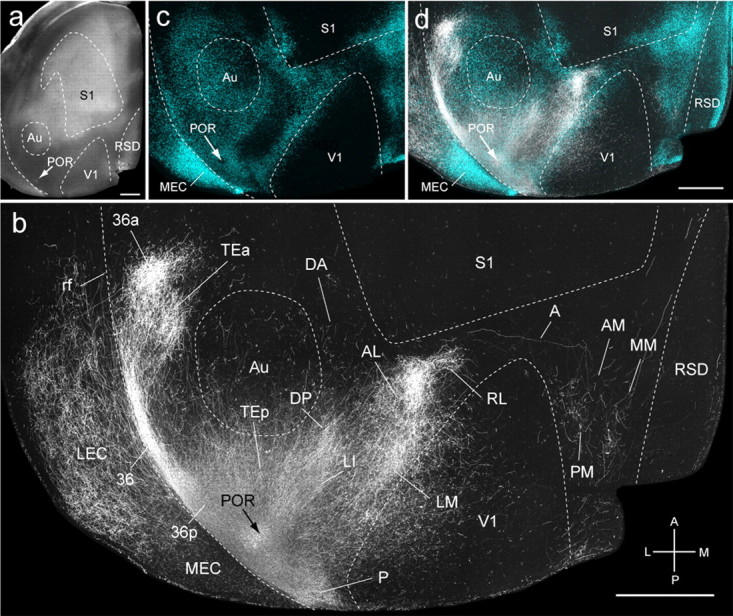
Connections of POR in tangential sections through flat-mounted mouse cerebral cortex. a, Dark-field image of wet-mounted, unstained section through layer 4 showing bright myelin-rich cortical fields. b, Dark-field image of anterogradely labeled axonal projections (white) after injection of BDA into POR (arrow). c, Blue labeling represents landmark pattern of retrogradely bisbenzimide-labeled callosal projection neurons. d, Overlay of callosal connections (blue) and BDA-labeled projections (white). Scale bars, 1 mm. Arrows indicate injection site.

Outputs of A

Three injections were made in the posterior parietal area A in the lateral parietal association cortex (Franklin and Paxinos, 2007), interposed between V1 and S1 (Fig. 3a,c). Each of these injections labeled 27 cortical projections. The projections within V1 marked subregions that confirmed the topographic organization of area A (Wang and Burkhalter, 2007). Unlike the projections of POR, most connections of area A terminated in anterior, medial, and dorsal cortices (Fig. 3b,d). Of the total weight of projections, 84% terminated in medial occipital, parietal, cingulate, frontal, and prefrontal cortices, whereas only 13% were destined for temporal, entorhinal, and piriform cortices (Fig. 4k). The dorsal bias was evident in the weak inputs to LM, LI, P, TEp, DP, Au, and the even sparser projections to POR, 36p, 36, and LEC (Figs. 3b, 4k). We found no inputs to MEC but some inputs to LEC and substantial inputs to the grid, head-direction, and border cell containing PrS (Franklin and Paxinos, 2007; Boccara et al., 2010). In contrast, inputs to AL, RL, S2, and the dorsal anterior auditory belt area (DA) contained within AuV (Franklin and Paxinos, 2007) were strong (Fig. 3b). Strong inputs were also found at topographically matching locations in barrels and septa of S1, whereas the projections to the trunk and limb representations of S1 were weak (Fig. 3b). Furthermore, strong projections were found in AM, PM, RSD, the neck representation of primary motor cortex (M1) (Franklin and Paxinos, 2007), the posterior whisker motor area (M2) (Brecht et al., 2004; Franklin and Paxinos, 2007), and the frontal eye field in Cg1 (Brecht et al., 2004) (Fig. 3b). Inputs to PrL, IL, and VO were weak.

Figure 3.

Connections of A in tangential sections through flat-mounted mouse cerebral cortex. a, Dark-field image of wet-mounted, unstained section through layer 4 showing bright myelin-rich cortical fields. b, Dark-field image of anterogradely labeled axonal projections (white) after injection of BDA into area A (arrow). c, Blue labeling represents landmark pattern of retrogradely bisbenzimide-labeled callosal projection neurons. d, Overlay of callosal connections (blue) and BDA-labeled projections (white). Scale bars, 1 mm. Arrows indicate injection site.

Nodes of the ventral stream

The ventrally biased connections suggested that areas LI and P may be nodes of the ventral stream. Indeed, 66% of LI inputs terminated in temporal and parahippocampal regions, whereas only 28% projected to occipital, parietal, medial, frontal, and cingulate cortices (Fig. 4c). The dorsoventral asymmetry was even stronger (74 vs 23%) for area P (Fig. 4d).

Area LI injections (n = 3) were located at the lateral posterior corner of the acallosal region lateral to V1 and labeled 33 cortical projections (Figs. 4c, 5a,c,d). In the example shown in Figure 5b, projections were biased to posterior V1, indicating that they originated from the upper visual field of LI. Projections to temporal cortex included LM, P, TEp, Au, DP, and DA, parahippocampal areas [POR, 36p, TEa, 35, MEC, LEC, PrS, parasubiculum (PaS)], the subiculum (Sub), and the subcortically located claustrum (Cl) (Fig. 4c). Projections to the medial, parietal, limbic, and orbitofrontal cortices included PM, MM, AL, RL, A, AM, S1, S2, RSD, RSG, Cg1, and VO. LI shared many connections with LM, but unlike LM, LI projected to S2 and auditory cortices (Au, DA, DP, TEp) (Fig. 4c).

Area P injections (n = 3) were located in acallosal cortex behind LM and labeled 34 cortical regions (Figs. 4d, 6a,c,d). In the example shown in Fig. 6b, inputs were biased to medial V1, indicating that P was topographically organized. Projections to LM and AL were weak and even sparser in PM, RL, A, and AM. The only strong input was to MM, which contrasted with sparse projections to RSD, RSG, Cg1, and the second cingulate area (Cg2) (Franklin and Paxinos, 2007), which in rat represents eye and periocular movements (Brecht et al., 2004) (Fig. 4d). In contrast, inputs to temporal (LI, TEp, Au, DP) and parahippocampal areas (POR, 36p, 36a, 35, MEC, PaS, PrS) were strong (Fig. 4d).

Nodes of the dorsal stream

The dorsally biased connections suggested that PM and the posterior parietal areas RL and AM are nodes of the dorsal stream. Indeed, each area showed a preference for dorsal over ventral targets: PM (64 vs 31%), RL (57 vs 35%), and AM (63 vs 30%) (Fig. 4g–i).

Area PM injections (n = 3) were located in the acallosal region posteromedial to V1 and labeled projections to 32 cortical regions (Figs. 4g, 7a,c,d). In the example shown in Figure 7b, projections were biased to posterior V1, indicating that PM is topographically organized. Although the connections favored dorsal over ventral areas, PM provided extensive inputs to temporal (LM, LI, P, TEp, Au, DP, DA) and parahippocampal (POR, TEa, 36p, 36a, 35, MEC, LEC, PaS, PrS) cortices. This ventral stream feature was also evident in the sparse input to S1 and S2 (Fig. 4g). However, the strong inputs to AL, AM, RL, A, MM, RSD, RSG, the eye and periocular motor areas (Cg1, Cg2) (Brecht et al., 2004), prefrontal cortex (PrL, IL), and VO suggest that PM projections favor the dorsal stream.

Figure 7.

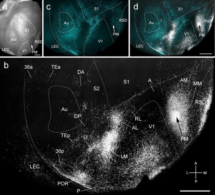
Connections of PM in tangential sections through flat-mounted mouse cerebral cortex. a, Dark-field image of wet-mounted, unstained section through layer 4 showing bright myelin-rich cortical fields. b, Dark-field image of anterogradely labeled axonal projections (white) after injection of BDA into area PM (arrow). c, Blue labeling represents landmark pattern of retrogradely bisbenzimide-labeled callosal projection neurons. d, Overlay of callosal connections (blue) and BDA-labeled projections (white). Scale bars, 1 mm. Arrows indicate injection site.

Area RL injections (n = 3) were associated with the small callosal ring near the tip of V1 and labeled 25 cortical projections (Figs. 4h, 8a,c,d). In the example shown in Figure 8b, inputs were biased to lateral V1, indicating that RL contains a visuotopic map. Inputs to LM and LI and the temporal areas (P, Au, DP, DA) were weak or completely absent in TEp. Similarly, sparse inputs were found in POR, 36p, 36a, 35, LEC, and PrS. In contrast, the projections to AL and PM were strong but sparse in MM. Inputs to S1 and S2 were notably strong and paralleled by projections to whisker motor (M2) (Brecht et al., 2004) and eye movement (Cg1) areas (Brecht et al., 2004).

Figure 8.

Connections of RL in tangential sections through flat-mounted mouse cerebral cortex. a, Dark-field image of wet-mounted, unstained section through layer 4 showing bright myelin-rich cortical fields. b, Dark-field image of anterogradely labeled axonal projections (white) after injection of BDA into area RL (arrow). c, Blue labeling represents landmark pattern of retrogradely bisbenzimide-labeled callosal projection neurons. d, Overlay of callosal connections (blue) and BDA-labeled projections (white). Scale bars, 1 mm. Arrows indicate injection site.

Area AM injections (n = 3) were located medial to the tip of V1 and labeled 30 cortical regions (Figs. 4i, 9a,c,d). In the example shown in Figure 9b, projections were in medial V1, indicating that AM contains a visuotopic map. Similar to PM and RL, AM provided strong or moderate input to LM, AL, PM, RL, and A. However, projections to S1, temporal (P, Au, DP, DA, TEp), and parahippocampal (POR, TEa, 36p, 36a, 35, LEC) cortices were weak or absent in MEC. The notable exception was the relatively strong projection to PrS, which in rat contains head, grid, and border cells (Boccara et al., 2010). This input was paralleled by projections to RSD and RSG, which are known to contain head direction cells (Taube, 2007). Strong inputs were also found to the periocular motor cingulate area (Cg1) and whisker motor cortex (M2).

Figure 9.

Connections of AM in tangential sections through flat-mounted mouse cerebral cortex. a, Dark-field image of wet-mounted, unstained section through layer 4 showing bright myelin-rich cortical fields. b, Dark-field image of anterogradely labeled axonal projections (white) after injection of BDA into area AM (arrow). c, Blue labeling represents landmark pattern of retrogradely bisbenzimide-labeled callosal projection neurons. d, Overlay of callosal connections (blue) and BDA-labeled projections (white). Scale bars, 1 mm. Arrows indicate injection site.

Connectivity profiles of dorsal and ventral nodes

The ordering of target areas by geographic location suggested that each source area has a unique distribution of projection strengths across different targets (Fig. 4). To further support this claim, we ordered projection targets by projection strengths. Figure 10 shows that the projections of each source area are distributed in a remarkably similar manner. Connection weights vary over two to three orders of magnitude, and distributions are well fit by a lognormal function. By comparison, the data are fit very poorly by normal (Gaussian) distributions. Furthermore, Figure 10 shows that, when connection weights are taken into account, each source area has a unique distribution of projection targets. In monkey, such source-specific target distributions were referred to as areal connectivity profiles (Markov et al., 2011). Most interestingly, when the source areas were ordered according to their dorsoventral location, we found that the connection strengths to ventral and dorsal areas progressively increased. These trends can be seen along the ventral stream by the gradual strengthening of connections to ventral areas (Fig. 10a–e, red boxes) and along the dorsal stream by the shift of dorsal areas (Fig. 10f–k, blue boxes) to the left of side of the graph.

Figure 10.

Projection densities are unique for each target area and follow a lognormal distribution. a–k, Circles and error bars represent the mean and SDs of individual measurements of optical density (same sample sizes as in Fig. 4), and projections are ordered by mean density for each of the 10 source areas under study. The curves represent an average over 10,000 random samples obtained from a log-normal distribution with the same mean and SD and an equal number of points as the data. The shaded area is defined by the 2.5 and 97.5 percentiles of the 10,000 samples. Colors at the bottom of each plot label the target areas by their association with the ventral (red) and dorsal (blue) streams.

Similarity structure of regional projections

The connection data consist of projection densities from 10 sources to 40 targets, which can be represented as 10 vectors of 40 observations (self-connections set to zero; Fig. 11a). Each area showed a unique pattern of projections. We assessed the between-area similarities of these projections using four approaches: the normalized dot product, k-means clustering, NMDS, and PCA. These analyses yielded similar projection patterns, with two sets of regions clustering together.

Figure 11.

Connection matrix and similarity structure. a, The matrix summarizes the density of projections (measured as optical density) from 10 source areas to 40 target areas. The submatrix M includes data on all reciprocal projections between the 10 areas at the extreme left of the plot. b, The normalized dot product matrix, a measure of the similarity of the projection patterns of the 10 areas plotted here. The matrix was reordered using an optimization algorithm to minimize distances (vector angles) between neighboring regions. c, Two-dimensional layout of connection patterns of areas V1, LM, LI, P, POR, AL, PM, RL, AM, and A after NMDS (stress = 0.0513). d, PCA. Layout in two principal dimensions capturing 36 and 14% of the variance, respectively.

We first calculated the vector angle (derived from the normalized dot product) for each pair of connection vectors, excluding mutual connections. The resulting similarity matrix was reordered to minimize entries near the main diagonal, thus arranging regions according to the similarity of their projection patterns (Fig. 11b). V1 was placed near the middle of the reordered matrix. Figure 11b shows that hot colors are clustered at opposite corners of the matrix, indicating greater similarity of connections among ventral or dorsal areas, and that the networks of ventral and dorsal areas are relatively distinct. k-means clustering was performed for two to five clusters, starting from 1000 random configurations and using the cosine of the vector angle as the distance metric. The Dunn's index was used to identify the clustering with maximal within-cluster coherence and between-cluster distance. The optimal partitions consisted of two clusters, one containing AL, RL, AM, PM, and A and the other containing V1, LM, LI, POR, and P. NMDS was performed using the vector angle between projections as distance measure. A configuration minimizing Kruskal's stress parameter separated AL, RL, AM, PM, and A from V1, LM, LI, POR, and P when data were projected onto two dimensions (Fig. 11c). PCA was performed on the correlation matrix of the projection patterns and resulted in dorsal and ventral clusters of areas similar to that found by NMDS (Fig. 11d). In both plots, V1 was more closely associated with the ventral stream, reflecting strong reciprocal connectivity with LM (Fig. 12a).

Figure 12.

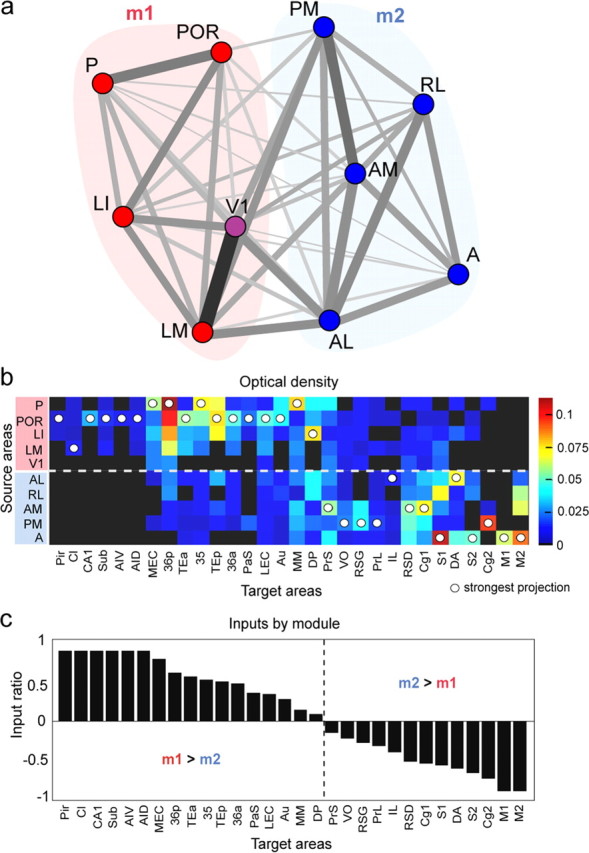
Modularity structure. a, Graphical layout of the connectivity of the submatrix M, after optimizing the position of the nodes (areas) using the Kamada–Kawai force-based energy minimization algorithm. Red areas belong to the ventral module m1. Blue areas belong to the dorsal module m2. V1 is more strongly affiliated with the ventral module and is colored in purple. Connections between pairs of areas are shown as the sum of their reciprocal projection density (darker gray/thicker lines = stronger projections). b, Projection density for 10 source regions to 30 projection areas, arranged by module origin (y-axis). White dots highlight the strongest projection each area receives. c, Ratio of inputs received from the two modules, computed as (Σm1 + Σm2)/(Σm1 − Σm2). A ratio of 1 indicates that the area receives inputs exclusively from module m1, and a ratio of −1 indicates inputs only from module m2. Areas are sorted by the magnitude of the ratio (x-axis).

Modularity and community structure

Using the connection matrix M (and M′) for the 10 reciprocally connected regions, we computed the optimal modularity partition and modularity score. For both M and M′, the optimal modularity partition split the regions into two communities, one comprising V1, LM, LI, POR, and P and the other AL, RL, AM, PM, and A. The proportion of within-module to between-module projections was 61–39%. To visualize the community structure, we displayed the connections of the 10 × 10 matrix after optimally arranging regions and connections with the Kamada–Kawai energy minimization layout algorithm (Kamada and Kawai, 1989) implemented in Pajek (http://pajek.imfm.si/). Figure 12a shows that the two communities have distinct patterns. We tested the significance of the modularity score by comparing to two different random populations (see Materials and Methods). The modularity score estimated from the empirical data was significantly greater than in the modularity found in both populations of randomized networks (p < 0.0001).

To reveal the projection strengths to destinations other than to the injected visuotopically organized areas (V1, LM, LI, P, POR, AL, PM, RL, A, AM), we replotted the inputs of the 10 source regions to 30 targets. Figure 12b shows that the strongest inputs from areas of the ventral module terminated in the hippocampus (CA1), the olfactory cortex (Pir), insular gustatory/visceral cortex [anterior ventral (AIV) and anterior dorsal (AID) insulas] (Franklin and Paxinos, 2007), the parahippocampal areas (MEC, LEC, Sub, PaS, 35, 36p, 36a), and the auditory areas (Au, TEp, DP). In contrast, areas of the dorsal module made stronger projections to the retrosplenial cortex (RSD, RSG), the somatosensory cortex (S1, S2), the prefrontal areas (PrL, IL), and the motor areas that control limb, whisker, and eye movements (M1, M2, Cg1, Cg2). These dorsoventral network asymmetries are even more striking in a plot of the normalized ratio of inputs from each module (Fig. 12c).

Paths and centrality

Two regions can exchange signals via direct or indirect paths. In weighted networks, indirect paths (passing through an intermediate node) can be “shorter” than those made by direct connections if their combined weights are strong. We found that, although the matrix of 10 regions was virtually fully connected, the shortest paths between two directed pairs of regions were often indirect. Figure 13a shows the distance matrix, derived after transforming connection weights to connection lengths using the inverse transform. Most short paths within the two modules represented direct connections. However, for many pairs located in different modules, the distance of the direct connection was longer than the path involving one intermediate step. Thus, although direct connections between modules offer potential paths, information may more effectively be exchanged through stronger indirect channels.

Figure 13.

Paths, distances, and centrality. a, Distance matrix recording the topological length of the shortest path between sources and targets, computed from the weighted submatrix M. White dots indicate matrix entries in which the shortest path corresponds to a direct connection between areas. All unmarked entries have path lengths of two or three steps, i.e., the shortest path passes through at least one intermediate node. Note that within-module paths are overwhelmingly direct, whereas many indirect paths are found for node pairs located in different modules. b, Betweenness centrality of visual regions in submatrix M, corresponding to the number of shortest paths that pass through each node. Areas LM and AL have highest betweenness centrality, whereas no shortest paths pass through area V1.

Nodes that serve as relays for many short paths may be considered hub nodes. These hubs can be identified by their betweenness centrality. Only 6 of 10 regions (LM, LI, POR, AL, PM, RL) participate in at least one of the short indirect paths (Fig. 13b), identifying the areas as integrative centers (Sporns, 2011) of unimodal and multimodal sensory inputs (Sporns et al., 2007). Notably, not a single short path linking the two modules traveled through V1, indicating that, similar to cat and monkey, V1 is not a network hub for inter-areal communication (Sporns et al., 2007). To control for the effect of node degree on centrality, we compared the regional betweenness centrality to that obtained from two different populations of random networks. LM had significantly greater centrality relative to both random models (p = 0.05; p = 0.01). Thus, LM is a central hub of the visual network. In monkey, this is a property of V4, which ranks higher in the hierarchy (Felleman and Van Essen, 1991; Coogan and Burkhalter, 1993).

Spatial embedding and wiring economy

From the area map (Fig. 1d), we estimated the average lengths of inter-areal pathways as Euclidean distances of the center-of-mass between different areas. Projection weights and lengths were inversely correlated (r = −0.51, p < 0.0001), indicating that nearby areas are more strongly linked. We calculated the total wiring cost as the sum of the product of connection weights and lengths. We then generated rewired connection matrices using the two random models. None of the rewired connection patterns had a lower wiring cost than the one found empirically (p < 0.0001). We then adopted a rewiring strategy that randomly permuted regional positions while keeping the connection topology unchanged. Analysis of 3,628,800 (10!) permutations yielded a total of 2278 configurations (0.06%) with a maximal improvement in wiring cost of 5.7%. Hence, although not strictly optimal, the spatial embedding of mouse visual cortex connectivity conserves wiring length.

Discussion

We traced the connections of 10 areas of mouse visual cortex and measured the optical densities (i.e., bouton densities; Wang et al., 2011) of efferent projections. Retrograde labeling and associated filling of local axon arbors was rare, accounting for a negligible 0.001–0.01% of the long-range projection strength (Helmstaedter et al., 2007). These measurements revealed a network with two modules, indicating that medial/anterior extrastriate visual areas (AL, RL, A, AM, PM) are more strongly linked to parietal, motor, and limbic cortices, whereas lateral extrastriate areas (LM, P, LI, POR) are preferentially connected to temporal and parahippocampal regions. This modularity coincides with the representation of visuospatial and object recognition functions in dorsal and ventral rat cortices (McDaniel et al., 1982; Kolb and Walkey, 1987; Ho et al., 2011) and suggests that visual information is processed in dorsal and ventral streams.

We have found that the cortical network in mice is more complex than reported in rat, showing that single areas have at least twice as many projection targets (Miller and Vogt, 1984; Reep et al., 1990; McDonald and Mascagni, 1996; Burwell and Amaral, 1998). Factors that may contribute to this apparent increase are that our search for projections was cortex-wide and our parsing of visual cortex was more extensive. As a result, we have assigned projections that in rat were thought to belong to a single cytoarchitectonic area (Miller and Vogt, 1984; Reep et al., 1990, 1994; Paperna and Malach, 1991) to multiple areas contained within this cytoarchitectonic region, which made the connectivity denser than presumed. Thus, without comparable area maps across species, it is difficult to determine how much denser the cortical graph in mice really is. Our results show that the 10 × 10 matrix of injected areas is 99% connected through dense short and sparser long-range connections at near-optimal wiring costs. The connectivity drops to 70 and 79% reciprocity in a 25 × 25 matrix of areas with direct input from V1. This is a 30% denser connectivity than estimated for visually related areas in monkey (Felleman and Van Essen, 1991; Markov et al., 2011).

Unlike previous studies, which showed that all corticocortical connections in rat are reciprocal (Vogt and Miller, 1983; Miller and Vogt, 1984), we found 20–40% unidirectional connections. We believe that this is a gross overestimate because cell body labeling with BDA was extremely sparse and iontophoretic injections clearly suboptimal for retrograde tracing of reciprocal connections (Jiang et al., 1993).

Many connections we have found in mice were identified previously in rat (Vogt and Miller, 1983; Miller and Vogt, 1984; Reep et al., 1990, 1994, 1996; Paperna and Malach, 1991; McDonald and Mascagni, 1996; Witter and Amaral, 2004; Agster and Burwell, 2009), which eliminates species or technical differences as explanations for streams. Although streams have been proposed previously in rats based on distinctive connections with the amygdala (McDonald and Mascagni, 1996), the detailed organization in mice was only revealed here by identifying visual areas (Wang and Burkhalter, 2007) and applying graph analysis to connection weights (Markov et al., 2011; Sporns, 2011). The analysis shows that the projection density of each source area varies over two to three orders of magnitude, which is only half the span found in the ∼200× larger monkey cortex (Markov et al., 2011). As in monkey (Markov et al., 2011), we found that the projection weights are distributed in log-normal manner. This suggests that the scaling of inter-areal connections is conserved across species and that the strength of interactions between areas may obey similar rules, assuming that information flow is captured by structural data (Binzegger et al., 2004). Moreover, our analysis shows that each visual area has a distinct connectivity profile (Markov et al., 2011), which orders areas by the weight of inputs. Importantly, we found that the order depends on the location of an area: the more ventral, the stronger the connections to ventral areas, and the more dorsal, the stronger the outputs to dorsal areas. This indicates that the visual cortical network in mice is organized into ventral and dorsal processing streams, reminiscent of the organization in cats and primates (Ungerleider and Mishkin, 1982; Hilgetag et al., 2000). Unsurprisingly, we found that the connections within streams are 22% stronger than between streams. However, connections across streams are abundant, and the shortest and thus presumably most effective paths connecting the two streams often go through distinct hubs (Sporns et al., 2007) such as LM and AL.

It is important to note that the network in mice differs from that in monkey. For example, in mice, V1 projects to all visual areas (Olavarria and Montero, 1989; this study), whereas in monkey, only V2, V3, V4, and middle temporal area MT receive input from V1 (Felleman and Van Essen, 1991). In addition, V1 in mice and rats sends input to somatosensory, retrosplenial, cingulate, orbitofrontal, temporal, and parahippocampal cortex (Vogt and Miller, 1983; Miller and Vogt, 1984; Reep et al., 1990, 1996; Burwell and Amaral, 1998), which in monkey are not directly connected to V1 (Felleman and Van Essen, 1991). In rats and mice, many V1 targets process somatosensory, auditory, and motor information (Wagor et al., 1980; Chen et al., 1994; Brett-Green et al., 2003; Brecht et al., 2004), suggesting that outputs from V1 are readily integrated with other modalities, a process that in monkey is performed only on outputs from higher areas. The difference may reflect the smaller number of hierarchical levels in rodent than primate visual cortex (Coogan and Burkhalter, 1993; Burkhalter and Wang, 2008).

The modular dorso/ventral structure of the network broadly agrees with lesion studies in rat, showing that damage of the ventral areas reduces visual acuity and object recognition but spares spatial orientation (McDaniel et al., 1982; Tees, 1999; Ho et al., 2011). In contrast, lesions in dorsal and medial areas disrupt visuospatial discrimination and navigation (Sánchez et al., 1997; Pinto-Hamuy et al., 2004; Save and Poucet, 2009). Fittingly, recent calcium imaging studies found that neuronal tuning to high-spatial frequency (SF) is more frequent in LI than in AL, RL, and AM, which are more selective for high-temporal frequency (TF) and the direction of motion (Andermann et al., 2011; Marshel et al., 2011), suggesting that ventral areas encode image detail, whereas dorsal areas encode visual motion (Van Essen and Gallant, 1994). However, the recordings also show that the organization is more complex. For example, in LM, the sensitivity for SF was low and many neurons were tuned to high TF (Marshel et al., 2011). This may not be surprising, given the dense connections of LM with dorsal and ventral areas. It suggests, however, that LM is a divided gateway to ventral and dorsal streams that may resemble monkey V2, which contains neurons with dorsal and ventral properties (Nassi and Callaway, 2009). Another surprise was that the dorsal stream area PM preferred ventral stream properties (Van Essen and Gallant, 1994), such as high SF, low TF, and slow speeds (Andermann et al., 2011; Marshel et al., 2011). That PM belongs to the dorsal stream is supported by the lack of connections with the amygdala (Wang and Burkhalter, 2011). However, PM receives strong inputs from V1, which may supply detailed information about the shape of slow-moving objects. Thus, as in monkey, the dorsal stream may have multiple branches specialized for the processing of visual information from self-motion and moving objects viewed from fixed locations (Kravitz et al., 2011).

PM stands out with strong projections to eye movement and attention centers in Cg2 and to the head direction cell-containing retrosplenial cortex (Muir et al., 1996; Brecht et al., 2004; Taube, 2007; this study). Interestingly, the head direction responses recorded in putative rat PM were found to be influenced by visual input (Chen et al., 1994), suggesting remapping of egocentric coordinates in an external, allocentric, reference frame. We found that areas RL, A, and AM are strongly reciprocally connected to S1, S2, cingulate, motor, and putative vestibular cortices within S2 (Nishiike et al., 2000). Each of these areas is highly sensitive to coarsely topographic, transient visual information (Andermann et al., 2011; Marshel et al., 2011) presumably generated by optic flow patterns during self-motion. The areal connectivity pattern suggests that these visual inputs are combined with somatosensory, proprioceptive, vestibular, and motor efferent copy signals, used for path integration. The network between both branches of the dorsal stream may link the internal path integration information with inputs from external landmarks and enable goal-directed navigation.

In rat, visual input to MEC is five times stronger than input to LEC (Kerr et al., 2007). We found that, in mice, MEC and LEC receive approximately equal input from the ventral stream, whereas dorsal stream inputs terminate mainly in LEC. Thus, unlike in rat (Deshmukh and Knierim, 2011), ventral “what” input flows to MEC and LEC, whereas dorsal “where” input to LEC is stronger. This organization supports the findings of object-responsive neurons and place-responsive neurons in LEC in the presence of local objects and suggests that LEC processes external landmark information (Deshmukh and Knierim, 2011).

References

- Agster KL, Burwell RD. Cortical efferents of the perirhinal, postrhinal, and entorhinal cortices in rat. Hippocampus. 2009;19:1159–1186. doi: 10.1002/hipo.20578. [DOI] [PMC free article] [PubMed] [Google Scholar]
- Andermann ML, Kerlin AM, Roumis DK, Glickfeld LL, Reid RC. Functional specialization of mouse higher visual cortical areas. Neuron. 2011;72:1025–1039. doi: 10.1016/j.neuron.2011.11.013. [DOI] [PMC free article] [PubMed] [Google Scholar]
- Binzegger T, Douglas RJ, Martin KAC. A quantitative map of the circuit of cat primary visual cortex. J Neurosci. 2004;24:8411–8453. doi: 10.1523/JNEUROSCI.1400-04.2004. [DOI] [PMC free article] [PubMed] [Google Scholar]
- Boccara CN, Sargolini F, Thoresen VH, Solstad T, Witter MP, Moser EI, Moser MB. Grid cells in the pre- and parasubiculum. Nat Neurosci. 2010;13:987–994. doi: 10.1038/nn.2602. [DOI] [PubMed] [Google Scholar]
- Brecht M, Krauss A, Muhammad S, Sinai-Esfahani L, Bellanca S, Margrie TW. Organization of rat vibrissa motor cortex and adjacent areas according to cytoarchitectonics, microstimulation, and intracellular stimuluation of identified cells. J Comp Neurol. 2004;479:360–373. doi: 10.1002/cne.20306. [DOI] [PubMed] [Google Scholar]
- Brett-Green B, Fifkov á E, Larue DT, Winer JA, Barth DS. A multisensory zone in rat parietotemporal cortex: intra-and extracellular physiology and thalamocortical connections. J Comp Neurol. 2003;460:223–237. doi: 10.1002/cne.10637. [DOI] [PubMed] [Google Scholar]
- Burkhalter A, Wang Q. Interconnections of visual cortical areas in the mouse. In: Chalupa LM, Williams RW, editors. Eye, retina, and visual system of the mouse. Cambridge, MA: Massachusetts Institute of Technology; 2008. pp. 245–254. [Google Scholar]
- Burwell RD, Amaral DG. Cortical afferents of the perirhinal, postrhinal, and entorhinal cortices of the rat. J Comp Neurol. 1998;398:179–205. doi: 10.1002/(sici)1096-9861(19980824)398:2<179::aid-cne3>3.0.co;2-y. [DOI] [PubMed] [Google Scholar]
- Chen LL, Lin LH, Barnes CA, McNaughton BL. Head-direction cells in the rat posterior cortex. II. Contributions of visual and ideothetic information to the directional firing. Exp Brain Res. 1994;101:24–34. doi: 10.1007/BF00243213. [DOI] [PubMed] [Google Scholar]
- Coogan TA, Burkhalter A. Hierarchical organization of areas in rat visual cortex. J Neurosci. 1993;13:3749–3772. doi: 10.1523/JNEUROSCI.13-09-03749.1993. [DOI] [PMC free article] [PubMed] [Google Scholar]
- Deshmukh SS, Knierim JJ. Representation of non-spatial and spatial information in the lateral entorhinal cortex. Front Behav Neurosci. 2011;5:69. doi: 10.3389/fnbeh.2011.00069. [DOI] [PMC free article] [PubMed] [Google Scholar]
- Felleman DJ, Van Essen DC. Distributed hierarchical processing in the primate cerebral cortex. Cereb Cortex. 1991;1:1–47. doi: 10.1093/cercor/1.1.1-a. [DOI] [PubMed] [Google Scholar]
- Franklin BJ, Paxinos G. The mouse brain in stereotaxic coordinates. Amsterdam: Elsevier; 2007. [Google Scholar]
- Frost DO, Caviness VS., Jr Radial organization of thalamic projections to the neocortex in the mouse. J Comp Neurol. 1980;194:369–393. doi: 10.1002/cne.901940206. [DOI] [PubMed] [Google Scholar]
- Gao E, DeAngelis GC, Burkhalter A. Parallel input channels to mouse primary visual cortex. J Neurosci. 2010;30:5912–5926. doi: 10.1523/JNEUROSCI.6456-09.2010. [DOI] [PMC free article] [PubMed] [Google Scholar]
- Girvan M, Newman ME. Community structure in social ad biological networks. Proc Natl Acad Sci U S A. 2002;99:7821–7826. doi: 10.1073/pnas.122653799. [DOI] [PMC free article] [PubMed] [Google Scholar]
- Goodale MA, Milner AD. Separate visual pathways for perception and action. Trends Neurosci. 1992;15:20–25. doi: 10.1016/0166-2236(92)90344-8. [DOI] [PubMed] [Google Scholar]
- Helmstaedter M, de Kock CP, Feldmeyer D, Bruno RM, Sakmann B. Reconstruction of an average cortical column in silico. Brain Res Rev. 2007;55:193–203. doi: 10.1016/j.brainresrev.2007.07.011. [DOI] [PubMed] [Google Scholar]
- Hilgetag CC, Burns GA, O'Neill MA, Scannell JW, Young MP. Anatomical connectivity defines the organization of clusters of cortical areas in the macaque monkey and the cat. Philos Trans R Soc Lond B Biol Sci. 2000;355:91–110. doi: 10.1098/rstb.2000.0551. [DOI] [PMC free article] [PubMed] [Google Scholar]
- Ho JW, Narduzzo KE, Outram A, Tinsley CJ, Henley JM, Warburton EC, Brown MW. Contributions of area Te2 to rat recognition memory. Learn Mem. 2011;18:493–501. doi: 10.1101/lm.2167511. [DOI] [PMC free article] [PubMed] [Google Scholar]
- Jiang X, Johnson RR, Burkhalter A. Visualization of dendritic morphology of cortical projection neurons by retrograde labeling. J Neurosci Methods. 1993;50:45–60. doi: 10.1016/0165-0270(93)90055-v. [DOI] [PubMed] [Google Scholar]
- Kamada T, Kawai S. An algorithm for drawing general undirected graphs. Inform Process Lett. 1989;31:7–15. [Google Scholar]
- Kerr KM, Agster KL, Furtak SC, Burwell RD. Functional neuroanatomy of the parahippocampal region: the lateral and medial entorhinal areas. Hippocampus. 2007;17:697–708. doi: 10.1002/hipo.20315. [DOI] [PubMed] [Google Scholar]
- Kolb B. Posterior parietal and temporal association cortex. In: Kolb B, Tees RC, editors. The cerebral cortex of the rat. Cambridge, MA: Massachusetts Institute of Technology; 1990. pp. 459–471. [Google Scholar]
- Kolb B, Walkey J. Behavioral and anatomical studies of the posterior parietal cortex in the rat. Behav Brain Res. 1987;23:127–145. doi: 10.1016/0166-4328(87)90050-7. [DOI] [PubMed] [Google Scholar]
- Kolb B, Buhrmann K, McDonald R, Sutherland RJ. Dissociation of the medial prefrontal, posterior parietal, and posterior temporal cortex for spatial navigation and recognition memory in the rat. Cereb Cortex. 1994;4:664–680. doi: 10.1093/cercor/4.6.664. [DOI] [PubMed] [Google Scholar]
- Kravitz DJ, Saleem KS, Baker CI, Mishkin M. A new neural framework for visuospatial processing. Nat Rev Neurosci. 2011;12:217–230. doi: 10.1038/nrn3008. [DOI] [PMC free article] [PubMed] [Google Scholar]
- Livingstone M, Hubel D. Segregation of form, color, movement, and depth: anatomy, physiology, and perception. Science. 1988;240:740–749. doi: 10.1126/science.3283936. [DOI] [PubMed] [Google Scholar]
- Markov NT, Misery P, Falchier A, Lamy C, Vezoli J, Quilodran R, Gariel MA, Giroud P, Ercsey-Ravasz M, Pilaz LJ, Huissoud C, Barone P, Dehay C, Toroczkai Z, Van Essen DC, Kennedy H, Knoblauch K. Weight consistency specifies regularities of macaque cortical networks. Cereb Cortex. 2011;21:1254–1272. doi: 10.1093/cercor/bhq201. [DOI] [PMC free article] [PubMed] [Google Scholar]
- Marshel JH, Garrett ME, Nauhaus I, Callaway EM. Functional specialization of seven mouse visual cortical areas. Neuron. 2011;72:1040–1054. doi: 10.1016/j.neuron.2011.12.004. [DOI] [PMC free article] [PubMed] [Google Scholar]
- Maslov S, Sneppen K. Specificity and stability of protein networks. Science. 2002;296:910–913. doi: 10.1126/science.1065103. [DOI] [PubMed] [Google Scholar]
- McDaniel WF, Coleman J, Lindsay JF., Jr comparison of lateral peristriate and striate neocortical ablations in the rat. Behav Brain Res. 1982;6:249–272. doi: 10.1016/0166-4328(82)90027-4. [DOI] [PubMed] [Google Scholar]
- McDonald AJ, Mascagni F. Cortico-cortical and cortico-amygdaloid projections of the rat occipital cortex: a Phaseolus vulgaris leucoagglutinin study. Neuroscience. 1996;71:37–54. doi: 10.1016/0306-4522(95)00416-5. [DOI] [PubMed] [Google Scholar]
- McNaughton BL, Leonard BJ, Chen L. Cortical-hippocampal interactions and cognitive mapping: a hypothesis based on reintegration of the parietal and inferotemporal pathways for visual processing. Psychobiology. 1989;17:236–246. [Google Scholar]
- Miller MW, Vogt BA. Direct connections of rat visual cortex with sensory, motor, and association cortices. J Comp Neurol. 1984;226:184–202. doi: 10.1002/cne.902260204. [DOI] [PubMed] [Google Scholar]
- Muir JL, Everitt BJ, Robbins TW. The cerebral cortex of the rat and visual attention function: dissociable effects of mediofrontal, cingulate, anterior dorsolateral, and parietal cortex lesions on a five-choice serial reaction time task. Cereb Cortex. 1996;6:470–481. doi: 10.1093/cercor/6.3.470. [DOI] [PubMed] [Google Scholar]
- Nassi JJ, Callaway EM. Parallel processing strategies of the primate visual system. Nat Rev Neurosci. 2009;10:360–372. doi: 10.1038/nrn2619. [DOI] [PMC free article] [PubMed] [Google Scholar]
- Nishiike S, Guldin WO, Bäurle J. Corticofugal connections between the cerebral cortex and the vestibular nuclei in the rat. J Comp Neurol. 2000;420:363–372. [PubMed] [Google Scholar]
- Olavarria J, Montero VM. Organization of visual cortex in the mouse revealed by correlating callosal and striate-extrastriate connections. Vis Neurosci. 1989;3:59–69. doi: 10.1017/s0952523800012517. [DOI] [PubMed] [Google Scholar]
- Paperna T, Malach R. Patterns of sensory intermodality relationships in the cerebral cortex. J Comp Neurol. 1991;308:432–456. doi: 10.1002/cne.903080310. [DOI] [PubMed] [Google Scholar]
- Pinto-Hamuy T, Montero VM, Torrealba F. Neurotoxic lesion of anteromedial/posterior parietal cortex disrupts spatial maze memory in blind rats. Behav Brain Res. 2004;153:465–470. doi: 10.1016/j.bbr.2004.01.003. [DOI] [PubMed] [Google Scholar]
- Reep RL, Goodwin GS, Corwin JV. Topographic organization in the corticocortical connections of medial agranular cortex in rats. J Comp Neurol. 1990;294:262–280. doi: 10.1002/cne.902940210. [DOI] [PubMed] [Google Scholar]
- Reep RL, Chandler HC, King V, Corwin JV. Rat posterior parietal cortex: topography of corticocortical and thalamic connections. Exp Brain Res. 1994;100:67–84. doi: 10.1007/BF00227280. [DOI] [PubMed] [Google Scholar]
- Reep RL, Corwin JV, King V. Neuronal connections of orbital cortex in rats: topograpghy of cortical and thalamic afferents. Exp Brain Res. 1996;111:215–232. doi: 10.1007/BF00227299. [DOI] [PubMed] [Google Scholar]
- Rubinov M, Sporns O. Complex network measures of brain connectivity: uses and interpretations. Neuroimage. 2010;52:1059–1069. doi: 10.1016/j.neuroimage.2009.10.003. [DOI] [PubMed] [Google Scholar]
- Salinas-Navarro M, Jiménez-López M, Valiente-Soriano FJ, Alarcón-Martínez L, Avilés-Trigueros M, Mayor S, Holmes T, Lund RD, Villegas-Pérez MP, Vidal-Sanz M. Retinal ganglion cell population in adult albino and pigmented mice: a computerized analysis of the entree population and its spatial distribution. Vis Res. 2009;49:637–647. doi: 10.1016/j.visres.2009.01.010. [DOI] [PubMed] [Google Scholar]
- Sánchez RF, Montero VM, Espinoza SG, Díaz E, Canitrot M, Pinto-Hamuy T. Visuospatial discrimination deficit in rats after ibotenic lesions in anteromedial visual cortex. Physiol Behav. 1997;62:989–994. doi: 10.1016/s0031-9384(97)00201-1. [DOI] [PubMed] [Google Scholar]
- Save E, Poucet B. Role of the parietal cortex in long-term representation of spatial information. Neurobiol Learn Mem. 2009;91:172–178. doi: 10.1016/j.nlm.2008.08.005. [DOI] [PubMed] [Google Scholar]
- Schneider GE. Two visual systems. Science. 1969;163:895–902. doi: 10.1126/science.163.3870.895. [DOI] [PubMed] [Google Scholar]
- Simmons PA, Lemmon V, Pearlman AL. Afferent and efferent connections of the striate and extrastriate visual cortex of the normal and reeler mouse. J Comp Neurol. 1982;211:295–308. doi: 10.1002/cne.902110308. [DOI] [PubMed] [Google Scholar]
- Sporns O. Networks of the brain. Cambridge, MA: Massachusetts Institute of Technology; 2011. [Google Scholar]
- Sporns O, Honey CJ, Kötter R. Identification and classification of hubs in brain networks. PLoS One. 2007;2:e104910. doi: 10.1371/journal.pone.0001049. [DOI] [PMC free article] [PubMed] [Google Scholar]
- Taube JS. The head direction signal: origins and sensory-motor integration. Annu Rev Neurosci. 2007;30:181–207. doi: 10.1146/annurev.neuro.29.051605.112854. [DOI] [PubMed] [Google Scholar]
- Tees RC. The effects of posterior parietal and posterior temporal cortical lesions on multimodal and nonspatial competencies in rats. Behav Brain Res. 1999;106:55–73. doi: 10.1016/s0166-4328(99)00092-3. [DOI] [PubMed] [Google Scholar]
- Ungerleider LG, Mishkin M. Two cortical systems. In: Ingle DJ, Goodale MA, Mansfield RJW, editors. Analysis of visual behavior. Cambridge, MA: Massachusetts Institute of Technology; 1982. pp. 549–586. [Google Scholar]
- Van Essen DC, Gallant JL. Neural mechanisms of form and motion processing in the primate visual system. Neuron. 1994;13:1–10. doi: 10.1016/0896-6273(94)90455-3. [DOI] [PubMed] [Google Scholar]
- Vogt BA, Miller MW. Cortical connections between rat cingulate and visual, motor, and postsubicular cortices. J Comp Neurol. 1983;216:192–210. doi: 10.1002/cne.902160207. [DOI] [PubMed] [Google Scholar]
- Wagor E, Mangini NJ, Pearlman AL. Retinotopic organization of striate and extrastriate visual cortex in the mouse. J Comp Neurol. 1980;193:187–202. doi: 10.1002/cne.901930113. [DOI] [PubMed] [Google Scholar]
- Wang Q, Burkhalter A. Area map of mouse visual cortex. J Comp Neurol. 2007;502:339–357. doi: 10.1002/cne.21286. [DOI] [PubMed] [Google Scholar]
- Wang Q, Burkhalter A. Steam-specific connections of mouse visual cortex with the amygdala. Soc Neurosci Abstr. 2011;38:378.02. [Google Scholar]
- Wang Q, Gao E, Burkhalter A. Gateways of ventral and dorsal streams in mouse visual cortex. J Neurosci. 2011;31:1905–1918. doi: 10.1523/JNEUROSCI.3488-10.2011. [DOI] [PMC free article] [PubMed] [Google Scholar]
- Witter PM, Amaral DG. Hippocampal formation. In: Paxinos G, editor. The rat nervous system. Amsterdam: Elsevier; 2004. pp. 637–687. [Google Scholar]