A Note on the Validity of Statistical Bootstrapping for Estimating the Uncertainty of Tensor Parameters in Diffusion Tensor Images

Abstract

Diffusion tensors are estimated from magnetic resonance images (MRIs) that are diffusion-weighted, and those images inherently contain noise. Therefore, noise in the diffusion-weighted images produces uncertainty in estimation of the tensors and their derived parameters, which include eigenvalues, eigenvectors, and the trajectories of fiber pathways that are reconstructed from those eigenvalues and eigenvectors. Although repetition and wild bootstrap methods have been widely used to quantify the uncertainty of diffusion tensors and their derived parameters, we currently lack theoretical derivations that would validate the use of these two bootstrap methods for the estimation of statistical parameters of tensors in the presence of noise. The aim of this paper is to examine theoretically and numerically the repetition and wild bootstrap methods for approximating uncertainty in estimation of diffusion tensor parameters under two different schemes for acquiring diffusion weighted images. Whether these bootstrap methods can be used to quantify uncertainty in some diffusion tensor parameters, such as fractional anisotropy (FA), depends critically on the morphology of the diffusion tensor that is being estimated. The wild and repetition bootstrap methods in particular cannot quantify uncertainty in the principal direction (PD) of isotropic (or oblate) tensor. We also examine the use of bootstrap methods in estimating tensors in a voxel containing multiple tensors, demonstrating their limitations when quantifying the uncertainty of tensor parameters in those locations. Simulation studies are also used to understand more thoroughly our theoretical results. Our findings raise serious concerns about the use of bootstrap methods to quantify the uncertainty of fiber pathways when those pathways pass through voxels that contain either isotropic tensors, oblate tensors, or multiple tensors.

I. Introduction

Because of the noise that is inherent in diffusion-weighted (DW) magnetic resonance images (MRIs), calculated diffusion tensors and their eigenspace components generally differ from the true ones, producing uncertainty in their estimation. Previous simulation studies have shown that estimated eigenvalues are always distinct and that their estimated fractional anisotropy (FA) is always greater than zero, regardless of whether the tensor is degenerate (i.e., oblate, prolate, or isotropic) or nondegenerate [1]–[4]. Thus, we always incorrectly identify the principal directions of tensors within regions that contain isotropic or oblate tensors. Furthermore, recent theoretical calculations have accurately approximated the uncertainty of the estimated eigenvalues and eigenvectors, as well as the bias that is introduced by sorting by their magnitudes eigenvalues in both degenerate and nondegenerate tensors [5], [6]. Those calculations have shown in particular that the uncertainty in identifying a tensor’s principal direction (PD) is determined primarily by whether the overall morphology of the tensor is degenerate or not [6].

Bootstrapping methods, including repetition and the wild bootstrap, have been widely used to quantify numerically the uncertainty of eigenvalues, eigenvectors, and fiber pathways that is caused by the presence of noise in DW images [7]–[11]. Repetition bootstrap in diffusion tensor imaging (DTI) requires repeated measurements in each gradient direction, because it resamples with replacement the raw DW images in each of those directions [7]. Numerical simulations have shown that the accuracy of the repetition bootstrap depends on the number of repeated measurements in each direction [12]. Instead of resampling the raw DW images, the wild bootstrap is a model-based method that resamples the residuals of the linear regression model used to estimate the tensor at each voxel. In particular, because use of the wild bootstrap is not limited to data from an acquisition scheme that acquires multiple measures in each gradient direction, it is applicable to most DTI acquisition schemes, including the standard acquisition of one measurement per direction, unlike the repetition bootstrap, which cannot be used when only one measure is acquired in each direction [9], [10].

Two fundamental questions remain regarding the correct use of bootstrap methods to quantify the uncertainty of tensor parameters: 1) Are bootstrap methods, such as the wild bootstrap, valid for quantifying the uncertainty of all DT parameters, regardless of tensor morphology? 2) Are bootstrap methods valid for quantifying the uncertainty of DT parameters in voxels containing multiple tensors? We will address these two questions systematically.

To address the first question, we will show that the wild and repetition bootstrap methods are invalid for quantifying the uncertainty of the parameters for some tensors, such as the principal direction of an isotropic or a degenerate tensor. Thus, to use these two bootstrap methods correctly, the morphology of a tensor must be known. The validity of the wild bootstrap strongly depends on the correct specification of the fitted model used to estimate a tensor. Because the wild bootstrap resamples the residuals of the fitted tensor model, resampled tensors may not reflect the true characteristics of DTs in real DW images. To the second question, the two bootstrap methods considered here may fail to quantify the parameters of a diffusion tensor in voxels containing multiple tensors. We examine these issues using both theoretical arguments and extensive Monte Carlo simulations.

II. Methods

A. Acquisition Schemes for Diffusion Tensor Imaging

Suppose that we have an acquisition scheme for acquiring MRI with multiple gradient directions and b factors, denoted by {(r_i, b_i) : i = 0, …, M}, where r_i = (r_i,1, r_i,2, r_i,3)^T is the ith gradient direction such that ${\mathbf{r}}_i^T{\mathbf{r}}_i=1$ and b_i is the corresponding b factor representing the magnitude of the diffusion gradients [5], [13], [14]. At each (r_i, b_i), we observe n_i measures of image intensities {S_ij : j = 1, …, n_i} for i = 0, …, M.

We focus on two commonly used DTI acquisition schemes, in which two different b values are chosen. For instance, we often set b₀ = 0 and b₁ = … = b_M = b s/mm². For notational simplicity, we henceforth assume that n₁ = … = n_M. When n₁ = … = n_M = 1, we obtain the most common DTI acquisition scheme that acquires one measurement per direction. If n₁ = … = n_M > 1, then we obtain the DTI acquisition scheme with multiple measurements per direction. In addition, we usually acquire more than one baseline image, so that n₀ > 1.

B. Bootstrap Methods for Single Tensor Model

Here, we assume that a single DT is present in each voxel. We therefore consider a single tensor model to fit log-transformed signal intensities log S_ij as follows:

$$\begin{array}{l}log{S}_{0k}=log{S}_0+{\eta }_{0k}\\ ={\mathbf{z}}_0^T\theta +exp\left(-{\mathbf{z}}_0^T\theta \right)\sigma {\epsilon }_{0k}\\ log{S}_{ij}=log{S}_0-b_i{\mathbf{r}}_i^T{\mathbf{Dr}}_i+{\eta }_{ij}\\ ={\mathbf{z}}_i^T\theta +exp\left(-{\mathbf{z}}_i^T\theta \right)\sigma {\epsilon }_{ij}\end{array}$$ (1)

for k = 1, …, n₀, i = 1, …, M and j = 1, …, n₁, where θ^T = (log S₀, (β^T) and D = (D_kl) is a 3×3 diffusion tensor, ${\eta }_{0k}=exp(-{\mathbf{z}}_0^T\theta )\sigma {\epsilon }_{0k},{\eta }_{ij}=exp(-{\mathbf{z}}_i^T\theta )\sigma {\epsilon }_{ij}$, and the errors ε_ij are independent random variables that have zero mean and finite variances. We define β^T = (D₁₁, D₁₂, D₁₃, D₂₂, D₂₃, D₃₃) and

$${\mathbf{z}}_i^T={(1,-b_i{(r_{i,1}^2,2r_{i,1}{r}_{i,2},2r_{i,1}{r}_{i,3},r_{i,2}^2,2r_{i,2}{r}_{i,3},r_{i,3}^2)}^T)}^T$$

for i = 0, …, M. We set r₀ = (1, 0, 0)^T and Var(ε₁) at 1 for identifiability purposes.

We consider the commonly used weighted least square (WLS) estimator [6], [15]. First, we calculate the ordinary least squares estimator as follows:

$$\begin{array}{l}{\widehat{\theta }}_{LS}={\left(n_0{\mathbf{z}}_0{\mathbf{z}}_0^T+\sum _{i=1}^M{n}_1{\mathbf{z}}_i{\mathbf{z}}_i^T\right)}^{-1}\\ \left({\mathbf{z}}_0\sum _{j=1}^{n_0}log{S}_{0j}+\sum _{i=1}^M{\mathbf{z}}_i\sum _{j=1}^{n_1}log{S}_{ij}\right).\end{array}$$ (2)

Then, we calculate the one-step WLS estimator of θ, denoted by θ̂ [5], [6], [9], [15]. Let ${\omega }_i=exp(2{\mathbf{z}}_i^T{\widehat{\theta }}_{\text{LS}})$ for i = 0, …, M, θ̂ is given by

$$\begin{array}{l}\widehat{\theta }={\left(n_0{\omega }_0{\mathbf{z}}_0{\mathbf{z}}_0^T+\sum _{i=1}^M{n}_1{\omega }_i{\mathbf{z}}_i{\mathbf{z}}_i^T\right)}^{-1}\\ \left({\mathbf{z}}_0\sum _{j=1}^{n_0}log{S}_{ij}+\sum _{i=1}^M{\omega }_i{\mathbf{z}}_i\sum _{j=1}^{n_1}log{S}_{ij}\right).\end{array}$$ (3)

Finally, we can obtain an unbiased estimator σ̂² of σ² given by

$$\frac{{\sum }_{j=1}^{n_0}{\left(log{S}_{0j}-{\mathbf{z}}_0^T\widehat{\theta }\right)}^2{\omega }_0+{\sum }_{i=1}^M{\sum }_{j=1}^{n_1}{\left(log{S}_{ij}-{\mathbf{z}}_i^T\widehat{\theta }\right)}^2{\omega }_i}{n_0+M{n}_1-7}.$$

Based on θ̂, we can obtain the weighted least squares estimator of β̂ or DT D̂, its eigenvalue and eigenvector pairs {(m_i, e_i) : i = 1, 2, 3} (m₁ ≥ m₂ ≥ m₃) and other DT parameters including FA [6], [7], [16]. Many tractography algorithms attempt to reconstruct fiber pathways by consecutively connecting the estimated principal directions (e₁)of the diffusion tensors in adjacent voxels [17], [18]. To test statistical inferences concerning tensor parameters, the “true” uncertainty or the asymptotic probability distributions of those parameters, including β̂ and {(m_i, e_i) : i = 1,2,3}, must be constructed.

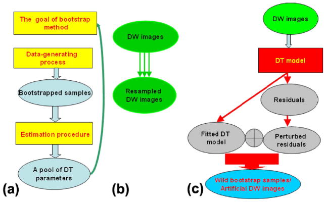
Bootstrap methods including the wild and repetition bootstraps are useful to construct the probability distributions of DT parameters accurately and precisely [7], [9], [10]. Any bootstrap method should explicitly specify its four components: its analytical goal, its method for generating data that compose the bootstrapped samples, its method for generating a pool of tensor parameters from those bootstrapped samples, and theoretical validation [Fig. 1(a)]. We explicitly specify the four components of the wild and repetition bootstraps for quantifying the uncertainty of β̂ and its parameters as follows. Our goal for bootstrapping in this study is to construct the probability distribution of the estimated β̂ in (3) and its related tensor parameters.

Fig. 1.

Graphical illustrations of bootstrap methods. (a) Four major components of a bootstrap method. (b) Data-generating process for generating repetition bootstrap samples. (c) Data-generating process for generating wild bootstrap samples.

We generate data for the bootstrap samples as follows [Fig. 1(b) and (c)]. To produce the B-th wild bootstrap sample { $(S_{ij;w}^B):i=0,\dots ,M;j=1,\dots ,n_i$}, we use the following data-generating process:

$$log{S}_{ij;w}^B={\mathbf{z}}_i^T\widehat{\theta }+exp\left(-{\mathbf{z}}_i^T\widehat{\theta }\right){\widehat{\epsilon }}_{ij}{\eta }_{ij}^{\ast }\widehat{\sigma }$$ (4)

where

$${\widehat{\epsilon }}_{ij}=\left[log{S}_{ij}-{\mathbf{z}}_i^T\widehat{\theta }\right]exp\left({\mathbf{z}}_i^T\widehat{\theta }\right)/(\widehat{\sigma }\sqrt{1-h_i})$$ (5)

in which $h_i={\mathbf{z}}_i^T{(n_0{\omega }_0{\mathbf{z}}_0{\mathbf{z}}_0^T+{\sum }_{i^{\prime }=1}^M{n}_1{\omega }_{i^{\prime }}{\mathbf{z}}_{i^{\prime }}{\mathbf{z}}_{i^{\prime }}^T)}^{-1}{\mathbf{z}}_i$, and ${\eta }_{ij}^{\ast }$ are independently and identically distributed as an F distribution, such as the standard normal distribution or the two-point distribution of Mammen [19], [20]. In the following, is chosen to be ±1 with equal probability [9], [21], [22]. Thus, the wild bootstrap only adds the perturbed residuals (5) back to the fitted DT model to produce the bootstrap sample [Fig. 1(c)]. It should be noted that the wild bootstrap can be applied with equal facility to the two DT acquisition schemes described above.

To generate the repetition bootstrap samples for DTI [7], we acquire N₀ − n₀ additional baseline images and N₁ − n₁ additional DW measurements for each gradient direction such that N₁ ≥ n₁. Then, we draw n₁ measurements with replacement from the N₁ measurements {S_ij : j = 1, …, N₁} for i = 1, …, M and n₀ measurements with replacement from the N₀ measurements {S_ij : j = l, … N₀} when b₀ = 0. Thus, we can create a repetition bootstrap sample { $S_{ij;r}^B:i=0,\dots ,M;j=1,\dots ,n_i$}. The repetition bootstrap can be applied to the two DT acquisition schemes described previously. After acquiring additional DW measurements, however, we must eventually consider the DT acquisition scheme that acquires multiple measures at each gradient direction, when n₁ > 1. If n₁ is much larger than 1, say n₁ = 10, then we can generate the repetition bootstrap sample by drawing n₁ measurements with replacement from the n₁ measurements {S_ij : j = 1, …, n₁} for the ith direction and n₀ measurements with the replacement from the n₀ baselines {S_0j : j = 1, …, n₀} at b₀ = 0.

We next need to produce a pool of tensor parameters from the bootstrap samples [Fig. 1(a)]. For the Bth wild bootstrap sample { $S_{ij;w}^B:i=0,\dots ,M;j=1,\dots ,n_i$}, we can calculate the weighted least squares estimator of DT ${\widehat{\mathbf{D}}}_w^B$, its eigenvalue and eigenvector pairs $\{(m_{i;w}^B,{\mathbf{e}}_{i;w}^B):i=1,2,3\}(m_{1;w}^B\ge m_{2;w}^B\ge m_{3;w}^B)$ and any other relevant DTI parameters. We repeat this process N_B (e.g., N_B = 10 000) times to obtain a pool of estimated DTI parameters. We can use this pool of DTI parameters to create their “probability distributions.” For example, we can use the pool of { $m_{1;w}^B:B=1,\dots ,N_B$} to approximate the uncertainty of m₁. The standard error of m_1;w can be approximated by the sample standard error of { $m_{1;w}^B:B=1,\dots ,N_B$} that is given by

$${\widehat{se}}_B=\sqrt{\sum _{B=1}^{N_B}{(m_{1;w}^B-{\overline{m}}_{1;w})}^2/(N_B-1)}$$

where ${\overline{m}}_{1;w}={\sum }_{B=1}^{N_B}{m}_{1;w}^B/N_B$. Furthermore, we may use the pool of { ${\mathbf{e}}_{1;w}^B:B=1,\dots ,N_B$} to construct the confidence cone of the principal direction. Similar to the wild bootstrap, we can create a pool of tensor parameters using all repetition bootstrap samples { $S_{ij;r}^B:i=0,\dots ,M;j=1,\dots ,n_i;B=1,\dots ,N_B$}.

The wild bootstrap differs substantially from the repetition bootstrap method [Fig. 1(b) and (c)]. The wild bootstrap, for example, always creates an artificial sample { $(S_{ij;w}^B):i=0,\dots ,M;j=1,\dots ,n_i$} based on the fitted DT model (4). Thus, { $(S_{ij;w}^B):i=0,\dots ,M;j=1,\cdots ,n_i$} only reflects the true characteristics of the fitted model. In general, if the fitted DT model cannot capture the true characteristics of real-world DW data within a voxel, then any statistical results based on the wild bootstrap sample may be incorrect. For instance, if we fit model (4) to DW data from a voxel that contains two tensors, then the wild bootstrap sample only reflects only the characteristics of the fitted single tensor model (4). Furthermore, assume that we fit model (4) to DW data from an isotropic tensor. Because the estimated DT D̂ is always nondegenerate [3], [6], the wild bootstrap sample reflects only the characteristics of that nondegenerate tensor D̂, whereas the repetition bootstrap always resamples the raw DW data and is therefore less sensitive to the assumptions of the fitted DT model than is the wild bootstrap, at least in the data-generating process.

C. Validating Bootstrap Methods

In this section, we use statistical results to validate the wild and repetition bootstraps for quantifying the uncertainty of diffusion tensor and its related tensor parameters. The noise inherent in DW images introduces uncertainty into the estimation of tensors, and the uncertainty of tensor parameters including the three eigenvalue and eigenvector pairs is determined primarily by the tensor morphology (degenerate or nondegenerate) [5], [6]. Although some DTs are in truth degenerate, estimated tensors are always nondegenerate because noise in real data will create some degree of inequality in a tensor’s eigenvalues, no matter how small. Measures that are derived from those eigenvalues and that are used to classify tensor morphologies also will be noise-laden and prone to error. The consequences of those errors in parameter estimates will vary depending on the true morphology of the tensor. The estimated principal direction of a tensor that is truly isotropic, for example, is uniformly distributed on the unit sphere, whereas it centers around the true principal direction for prolate and nondegenerate tensors [6]. Although we have derived the probability distributions of the estimated eigenvalues and eigenvectors given the prior knowledge of the true morphologies of these tensors [6], we generally do not have that prior knowledge when applying bootstrap methods to the statistically based classification of tensor morphology in real world datasets. Whether we can use bootstrap methods to quantify the uncertainty of the DT parameters without prior knowledge of a tensor’s true morphology in a real-world dataset is an important question. This question is critical for statistically validating the wild and repetition bootstraps for quantifying the uncertainty of β̂ and its tensor parameters.

To address this question, we must distinguish two types of tensor parameters. The first type includes all DT parameters that are continuously differentiable functions of the tensor β. These include all six elements of β, the trace of the tensor, FA and the relative anisotropy (RA) for anisotropic tensor, and three eigenvalue-eigenvector pairs for a nondegenerate tensor. All bootstrap methods are valid for this type of DT parameters. This statement can be established as follows. First, we can demonstrate the validity of quantifying the uncertainty of the estimated DT β based on the bootstrap methods discussed in Section II-B, [6], [8], [23]. Second, for any continuously differentiable function φ(β), if the first derivative of φ(β) does not equal zero, we apply the delta-method for bootstrap in probability to show the consistency of the bootstrap estimators [23]. This result guarantees the appropriateness of using the wild and repetition bootstrap methods to quantify the uncertainty of this first type of tensor parameters.

The second type includes all tensor parameters that are either not continuously differentiable functions of β or all tensor parameters whose first derivatives equal to zero. These include all the eigenvalues for degenerate tensors, the principal direction for oblate and isotropic tensors, and FA and RA for isotropic tensors. We cannot use our bootstrap methods in Section II-B to quantify the uncertainty of these DT parameters. For degenerate tensors, for example, we cannot use {m_i,B : i = 1, 2, 3} to approximate the uncertainty of the estimated eigenvalues or {e_1,B} to quantify the uncertainty of the estimated principal direction. We have previously shown theoretically that the bootstrap methods in Section II-B cannot produce the correct probability distributions of these tensor parameters, such as FA in isotropic tensor [6], [24].

These results suggest strongly that valid use of the bootstrap methods to quantify the uncertainty in estimating eigenvalue and eigenvector pairs of a tensor as well as FA and certain other tensor parameters is determined primarily by the morphology of the tensor. These considerations also raise a serious concern about the validity of bootstrapping those fiber pathways that pass through degenerate tensors, which account for about rougly 45% of all voxels in the brain [6], [25]. A natural question is therefore how to avoid the inappropriate use of the bootstrap methods in DTI analysis. One solution would be to classify tensor morphologies before the application of bootstrap procedures [6], [25], which would allow us to use information about the “true” tensor morphology of the tensors when approximating the probability distributions of the tensor parameters. An alternative solution would be to develop a “new” bootstrap method that does not require prior identification of tensor morphology.

D. Voxels With Multiple Tensors

Thus far our treatment of bootstrap methods has been limited to estimating tensor parameters when only a single tensor is present in each voxel. Developing bootstrap method for estimating parameters when multiple tensors are present within a single voxel, however, is also important [26]–[29], because DW images will always contain voxels with multiple tensors and these voxels will always challenge statistical models for tensor estimation and fiber tracking. How to develop a bootstrap method is primarily determined by the goal of bootstrap method [Fig. 1(a)].

Assume, for example, that the goal of bootstrapping is to determine the uncertainty of the estimated β̂ (or D̂) in (3) when employing a single tensor model. Although we may apply the same bootstrap methods to achieve this goal, as we have thus far, we are faced with the same vexing issue of requiring prior knowledge of the tensor’s true morphology. Thus, even though the voxel contains multiple tensors, it can be shown that there is a pseudo diffusion tensor, denoted by β_* or D_*, associated with the voxel that contains multiple tensors, and we could use this pseudotensor when testing statistical inferences, such as estimating the confidence interval of a tensor parameter [30]. To construct a confidence interval for tr(D_*), for example, we can show that $\sqrt{n_0+n_{1}M}(\text{tr}(\widehat{\mathbf{D}})-\text{tr}({\mathbf{D}}_{\ast }))$ converges statistically to a normal distribution with zero mean and variance ${\sigma }_{\text{tr}}^2$. Thus, given the value of ${\sigma }_{\text{tr}}^2$, a 95% confidence interval for tr(D_*) is given by [ $-1.96{\sigma }_{\text{tr}}/\sqrt{n_0+n_{1}M}+\text{tr}(\widehat{\mathbf{D}}),1.96{\sigma }_{\text{tr}}/\sqrt{n_0+n_{1}M}+\text{tr}(\widehat{\mathbf{D}})$]. If the pseudo tensor D_* is degenerate, we may not quantify the uncertainty of various DT parameters (e.g., the principal direction) derived from β̂ in (3) (see simulation study in Section III).

Fiber tracking is invalid when using a single tensor model and samples generated by wild and repetition bootstrapping when fiber tracts in fact pass through voxels containing multiple tensors. We emphasize that the pseudotensor D_*, which is a combination of all tensors within the voxel, may not resemble any of these tensors in that voxel. Because most fiber tracking algorithms can only track fibers using the principal direction of in D_* the voxel containing multiple tensors, probabilistic fiber tracking that is based on wild and repetition bootstrap samples do not convey any information about the “true” fiber pathway. To construct probabilistic fiber pathways, we need instead to determine the number of tensors in the voxel and then accurately estimate each tensor within that voxel. These remain daunting problems that require further research.

III. Monte Carlo Simulations

A. Single Tensor Voxels

We assessed the performance of the repetition and wild bootstrap methods methods for estimating confidence intervals of degenerate and nondegenerate tensors. We generated the simulated diffusion-weighted images as follows. We set at S₀ 1500 and σ₀ = 75 to obtain a signal-to-noise ratio (SNR = S₀/σ₀) 20 for all Monte Carlo simulations. In all simulation studies, we used four diagonal diffusion tensors D_i (i = 1, 2, 3, 4), whose three diagonal elements were, respectively, [0.7, 0.7, 0.7], [0.8, 0.8, 0.5], [1.1, 0.5, 0.5], and [0.9,0.7, 0.5] (units: 10⁻³ mm²/s). The shapes of the four diffusion tensors D_i (i = 1, 2, 3, 4) were, respectively, isotropic, oblate, prolate, and nondegenerate. For each i, the mean diffusivity λ̄ = tr(D_i)/3 was set equal to 0.7 × 10⁻³ mm²/s, a value typical in the human brain [5], [31].

For a given diffusion tensor D, x_i and y_i were generated from a Gaussian random generator with mean zero and standard deviation σ₀. Then we calculated $S_i=\sqrt{{(S_{0}exp(-b_i{\mathbf{r}}_i^T\mathbf{D}{\mathbf{r}}_i)+x_i)}^2+y_i^2}$ as the resulting diffusion-weighted data at the ith acquisition. For each diffusion tensor, 10 000 diffusion weighted datasets were simulated, which we used to calculate the weighted least squares estimates β̂ and their eigenvalue-eigenvector pairs {{m_j, e_j) : j = 1, 2, 3}. Those 10 000 sets of DTI parameters provided a gold standard for evaluating different bootstrap methods.

To evaluate the performance of the bootstrap methods in estimating the confidence intervals (or cones) of tensor parameters, we took a DW dataset for each diffusion tensor at SNR = 20, and then we generated the 10 000 bootstrap samples for each bootstrap method using a DW dataset for each tensor at SNR = 20. Finally, for each of the 10 000 bootstrap samples, we calculated the weighted least squares estimates β̂ and their eigenvalue-eigenvector pairs {{m_j, e_j) : j = 1, 2, 3}. Because some simulation studies of FA have been reported previously [9], [10], we primarily examined the use of bootstrap methods to reconstruct the probability distribution of the principal direction, which plays a critical role in any fiber tracking algorithm.

We considered a DT acquisition scheme having m = 1000 base-line images and n − m = 60 DW images at b = 1000 s/mm². The DT acquisition included ten measurements for each direction and the six gradient directions were arranged uniformly in 3-D space. For the repetition bootstrap, we drew 10 measures with replacement from the 10 measurements for each direction and 10 measurements from the 10 measures when b₀ = 0. For the wild bootstrap, we used the data-generating process previously described (4). We also studied the DT acquisition scheme having only a single measurement in each gradient direction. For the sake of space, we include these results in a supplementary document.

B. Voxels With Two Tensors

We further considered the performance of the two bootstrap methods in estimating confidence intervals (or cones) of diffusion tensor parameters when two tensors are allowed to cross within a single voxel. We generated the DW data for a voxel in which its signal contains components from two different fibers

$$S_0\left[fexp\left(-b_i{r}_i^T{\mathbf{D}}_5{r}_i\right)+(1-f)exp\left(-b_i{r}_i^T{\mathbf{D}}_6{r}_i\right)\right]$$ (6)

where f ∈ [0,1] and 1 − f are the signal fractions of the DTs D₅ and D₆. We added complex Gaussian noise having a standard deviation σ₀ to the simulated real channel signal. We set S₀ = 1500 and σ₀ = 75. We chose a rich-shaped tensor in white matter (WM) for D₅ = [λ₁, λ₂, λ₃] = [1.4, 0.35, 0.35], while we considered two DTs for D₆ that represented white matter [0.35, 1.4, 0.35] and gray matter (GM) [0.7, 0.7, 0.7] (units: 10⁻³ mm²/s). Thus, two combinations of D₅ and D₆ were studied: 1) WM + WM and 2) WM + GM. For WM+WM combination, the angle between the principal directions of D₅ and D₆ was set to 90°. We studied two differing values for f: f = 0.5 and 0.25. Then we repeated the Monte Carlo simu­lations for the single tensor case in Section III.

IV. Results

A. Single Tensor Voxels

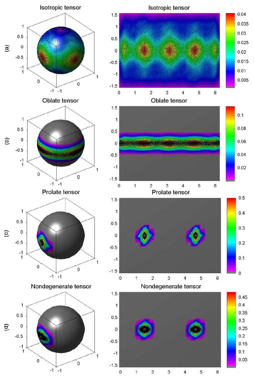
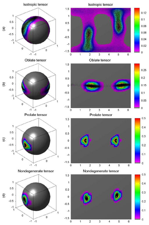
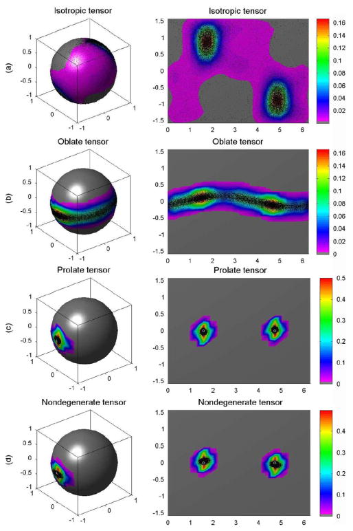
We generated the probability distributions for the principal eigenvectors for each tensor based on simulations using 10 000 DW images, 10 000 repetition bootstrap samples, and 10 000 wild bootstrap samples at SNR = 20 (Figs. 2–4). The true probability distribution of the principal direction for the isotropic tensor D₁ was distributed uniformly on the unit sphere [Fig. 2(a)], whereas the distribution for the oblate tensor D₂ encircled the sphere in a narrow belt [Fig. 2(b)]. The true probability distributions of the principal directions for the prolate and nondegenerate tensors centered on their true principal directions [Fig. 2(c) and (d)]. Consistent with the considerations presented in Section II-C, the wild and repetition bootstrap methods produced good estimates of the probability distributions of the principal eigenvectors for the prolate and nondegenerate tensors, whereas they were unable to estimate the probability distributions of the principle eigenvector for the isotropic and oblate tensors (Figs. 3–4). As expected, the probability distributions estimated using the wild bootstrap for the principal direction of all four tensor types always clustered around two opposite directions, regardless of the true morphology of the tensor, because wild bootstrap samples were generated from the fitted tensor model assuming a nondegenerate D̂. In contrast, the repetition bootstrap produced a more accurate estimate of the probability distribution of principal eigenvector than did the wild bootstrap for the oblate tensor (Figs. 2–4).

Fig. 2.

Golden standard for single tensor voxels: (a) the probability distributions of the principal directions from 10 000 simulated DW datasets for isotropic tensor, (b) oblate tensor, (c) prolate tensor, and (d) nondegenerate tensor, respectively. In each panel, the first column is the spherical representation of the principal eigenvectors, whereas the second column is the polar plot of the principal eigenvectors. The color codes suggest the local density of the simulated points: white circle represents the true principal direction and black dots represents simulated principal directions.

Fig. 4.

Wild bootstrap for single tensor voxels: (a) the probability distributions of the principal directions from 10 000 wild bootstrap samples for isotropic tensor, (b) oblate tensor, (c) prolate tensor, and (d) nondegenerate tensor, respectively. In each panel, the first column is the spherical representation of the principal eigenvectors, whereas the second column is the polar plot of the principal eigenvectors. The color codes suggest the local density of the simulated points: white circle represents the true principal direction and black dots represents simulated principal directions.

Fig. 3.

Repetition bootstrap for single tensor voxels: (a) the probability distributions of the principal directions from 10 000 repetition bootstrap samples for isotropic tensor, (b) oblate tensor, (c) prolate tensor, and (d) nondegenerate tensor, respectively. In each panel, the first column is the spherical representation of the principal eigenvectors, whereas the second column is the polar plot of the principal eigenvectors. The color codes suggest the local density of the simulated points: white circle represents the true principal direction and black dots represents simulated principal directions.

B. Voxels With Two Tensors

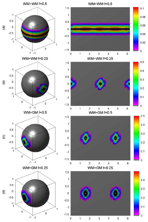
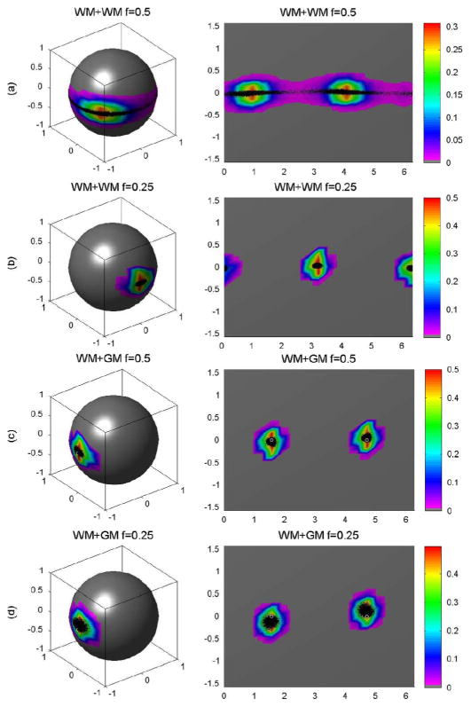
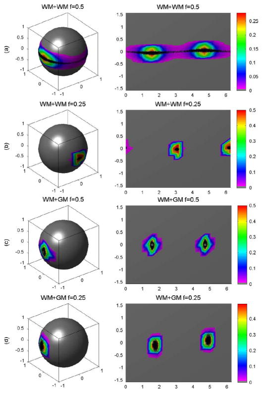
When using a single tensor model (4), the estimated D̂ cannot recover the two tensor components present within the DW images; however, the estimated D̂ in that instance then approximates a pseudo tensor, D_* = fD₅ + (1 − f)D₆, which is the weighted sum of the two tensors D₅ and D₆ [32]. When f = 0.5, neither D₅ nor D₆ dominates the voxel, whereas D₆ dominates the two-DT model at f = 0.25. For two tensor WM + WM combination, the three eigenvalues of D_* are given by λ_1,p = 1.4(1 − f) + 0.35f, λ_2,p = 0.35(1 − f) + 1.4f, and λ _3,p = 0.35f + 0.35(1 − f), respectively. At f = 0.5, we had λ_1,p = 0.875, λ_2,p = 0.875, and λ_3,p = 0.35. Thus, we expected to estimate an oblate pseudo DT. At f = 0.25, however, the principal direction of D_* is (0, 1, 0) and the three eigenvalues of D_* are given by 1.1375, 0.6125, and 0.35, respectively. For the WM + WM combination, the principal direction of D_* is not the same as the principal directions of D₅ or D₆. Similarly, for the WM + GM combination, the three eigenvalues of D_* are given by 1.05, 0.525, and 0.525 at f = 0.5 (0.875, 0.6125, 0.6125 at f = 0.25). For WM + GM, therefore, we expected to estimate a prolate pseudo tensor; moreover, the principal direction of D_* is the same as the principal direction of D₅ and therefore, the use of the principal direction of D_* cannot recover the principal direction of each tensor component within the voxel.

We simulated the principal eigenvectors from 10 000 DW images, 10 000 wild bootstrap samples, and 10 000 repetition bootstrap samples (Figs. 5–7). For the WM+WM combination and f = 0.5, the estimated principal directions created a band around the equator of the unit sphere [Fig. 5(a)]. For this WM + WM combination but with f = 0.25, the principal directions centered on (0, 1, 0) and (0, −1, 0) [Fig. 5(b)]. For the WM + GM combination and f = 0.5 or f = 0.25, the principal directions centered on (1, 0, 0) and (−1, 0, 0) [Fig. 5(c) and (d)]. The wild and repetition bootstrap methods produced similar results for WM+WM at f = 0.25 and WM+GM at f = 0.5 and 0.25 (Figs. 5–7), whereas they were unable to recover the principal directions of D₅ and D₆, the tensors of primary interest for fiber tracking. As expected, the wild and repetition bootstrap methods also could not generate the true uncertainty of the principal direction of D_* for WM + WM at f = 0.5 [Fig. 5(a), Fig. 6(a), and Fig. 7(a)].

Fig. 5.

Golden standard for voxels with two tensors: (a) the probability distributions of the principal directions from 10 000 simulated DW datasets for WM + WM and f = 0.5, (b) WM + WM and f = 0.25, (c) WM + GM and f = 0.5, and (d) WM + GM and f = 0.25, respectively. In each panel, the first column is the spherical representation of the principal eigenvectors, whereas the second column is the polar plot of the principal eigenvectors. The color codes suggest the local density of the simulated points: white circle repre­sents the true principal direction and black dots represents simulated principal directions.

Fig. 7.

Wild bootstrap for voxels with two tensors: (a) the probability distributions of the principal directions from 10 000 wild bootstrap samples for WM + WM and f = 0.5, (b) WM + WM and f = 0.25, (c) WM + GM and f = 0.5, and (d) WM + GM and f = 0.25, respectively. In each panel, the first column is the spherical representation of the principal eigenvectors, whereas the second column is the polar plot of the principal eigenvectors. The color codes suggest the local density of the simulated points: white circle represents the true principal direction and black dots represents simulated principal directions.

Fig. 6.

Repetition bootstrap for voxels with two tensors: (a) the probability distributions of the principal directions from 10 000 repetition bootstrap samples for WM + WM and f = 0.5, (b) WM + WM and f = 0.25, (c) WM + GM and f = 0.5, and (d) WM+GM f = 0.25, respectively. In each panel, the first column is the spherical representation of the principal eigenvectors, whereas the second column is the polar plot of the principal eigenvectors. The color codes suggest the local density of the simulated points: white circle represents the true principal direction and black dots represents simulated principal directions.

V. Discussion

We have presented a set of answers for two interrelated questions that are of central importance to the use of bootstrap methods in quantifying the uncertainty of tensor parameters. We have shown that the appropriate use of the wild and repetition bootstrap methods critically depends on the overall morphology of the tensor that is being estimated. We have shown in particular that quantifying the uncertainty of some diffusion tensor parameters, such as principal directions of isotropic and oblate tensors, is invalid when using these methods. We have demonstrated that the wild bootstrap is sensitive to the correct specification of the fitted tensor model. We have shown that use of bootstrap methods in voxel with multiple tensors cannot recover the principal direction of each tensor component within the voxel. Our findings suggest that use of the bootstrap methods to quantify the uncertainty of fiber pathways, when they pass through the voxels containing either oblate or isotropic tensors or multiple tensors, can be highly misleading. We have supported our findings using both simulation studies and statistical theory.

Many aspects of this work warrant further research. Perhaps the most pressing need is the development of new bootstrap methods that avoid the need for prior information of a tensor’s true morphology. The development of new statistical methods for determining the number of tensors in a voxel and for accurately estimating their individual tensor parameters is also of crucial importance to improve the validity of fiber tracking algorithms. Finally, the probabilistic construction of fiber tracts using statistical methods will also be important for determining the confidence with which tractography algorithms identify specific fiber tracts within the brain.

References

- 1.Pierpaoli C, Basser PJ. Toward a quantitative assessment of diffusion anisotropy. Magn Reson Med. 1996;36:893–906. doi: 10.1002/mrm.1910360612. [DOI] [PubMed] [Google Scholar]
- 2.Basser PJ, Pajevic S. Dealing with uncertainty in diffusion tensor MR data. Israel J Chem. 2003;43:129–144. [Google Scholar]
- 3.Basser PJ, Pajevic S. Statistical artifacts in diffusion tensor MRI (DT-MRI) caused by background noise. Magn Reson Med. 2000;44:41–50. doi: 10.1002/1522-2594(200007)44:1<41::aid-mrm8>3.0.co;2-o. [DOI] [PubMed] [Google Scholar]
- 4.Behrens TEJ, Woolrich MW, Jenkinson M, Johansen-Berg H, Nunes RG, Clare S, Matthews PM, Brady JM, Smith SM. Characterization and propagation of uncertainty in diffusion-weighted imaging. Magn Reson Med. 2003;50:1077–1088. doi: 10.1002/mrm.10609. [DOI] [PubMed] [Google Scholar]
- 5.Anderson AW. Theoretical analysis of the effects of noise on diffusion tensor imaging. Magn Reson Med. 2001;46:1174–1188. doi: 10.1002/mrm.1315. [DOI] [PubMed] [Google Scholar]
- 6.Zhu HT, Zhang HP, Ibrahim JG, Peterson B. Statistical analysis of diffusion tensors in diffusion-weighted magnetic resonance imaging Data (with discussion) J Amer Stat Assoc. 2007;102:1085–1102. [Google Scholar]
- 7.Pajevic S, Basser PJ. Parametric and non-parametric statistical analysis of DT-MRI Data. J Magn Reson. 2003;161:1–14. doi: 10.1016/s1090-7807(02)00178-7. [DOI] [PubMed] [Google Scholar]
- 8.Efron B, Tibshirani RJ. An Introduction to the Bootstrap. London, U.K: Chapman and Hall; 1993. [Google Scholar]
- 9.Whitcher B, Tuch DS, Wisco JJ, Sorenson AG, Wang L. Using the wild Bootstrap to quantify uncertainty in DTI. Human Brain Mapp. 2008;29:346–362. doi: 10.1002/hbm.20395. [DOI] [PMC free article] [PubMed] [Google Scholar]
- 10.Chung S, Liu Y, Henry RG. Comparison of bootstrap approaches for estimation of uncertainties of DTI parameters. NeuroImage. 2006;33:531–541. doi: 10.1016/j.neuroimage.2006.07.001. [DOI] [PubMed] [Google Scholar]
- 11.Lazar M, Alexander AL. Bootstrap white matter tractography (BOOT-TRAC) NeuroImage. 2005;24:524–532. doi: 10.1016/j.neuroimage.2004.08.050. [DOI] [PubMed] [Google Scholar]
- 12.O’Gorman RL, Jones DK. Just how much data need to be collected for reliable bootstrap DT-MRI? Magn Reson Med. 2006;56:884–890. doi: 10.1002/mrm.21014. [DOI] [PubMed] [Google Scholar]
- 13.Stejskal EO, Tanner JE. Spin diffusion measurements: Spin echoes in the presence of a time-dependent field gradient. J Chem Phys. 1965;42:288–292. [Google Scholar]
- 14.Kingsley PB. Introduction to diffusion tensor imaging mathematics: Part II. Anisotropy, diffusion-weighting factors, and gradient encoding schemes. Concepts Magn Reson. 2006;28A(pt A):123–154. [Google Scholar]
- 15.Basser PJ, Mattiello J, LeBihan D. Estimation of the effective self-diffusion tensor from the NMR spin echo. J Magn Reson, ser B. 1994;103:247–254. doi: 10.1006/jmrb.1994.1037. [DOI] [PubMed] [Google Scholar]
- 16.Salvador R, Pena A, Menon DK, Carpenter TA, Pickard JD, Bullmore ET. Formal characterization and extension of the linearized diffusion tensor model. Human Brain Mapp. 2005;24:144–155. doi: 10.1002/hbm.20076. [DOI] [PMC free article] [PubMed] [Google Scholar]
- 17.Conturo TE, Lori NF, Cull TS, Akbudak E, Snyder A, Shimony JS, McKinstry RC, Burton H, Raichle ME. Tracking neuronal fiber pathways in the living human brain. Proc Nat Acad Sci USA. 1999;96:10422–10427. doi: 10.1073/pnas.96.18.10422. [DOI] [PMC free article] [PubMed] [Google Scholar]
- 18.Xu D, Mori S, Solaiyappan M, van Zijl PC, Davatzikos C. A framework for callosal fiber distribution analysis. NeuroImage. 2002;17:1131–1143. doi: 10.1006/nimg.2002.1285. [DOI] [PubMed] [Google Scholar]
- 19.Liu RY. Bootstrap procedure under some non-i.i.d. models. Ann Stat. 1988;16:1696–1708. [Google Scholar]
- 20.Mammen E. Bootstrap and wild bootstrap for high dimensional linear models. Ann Stat. 1993;21:255–285. [Google Scholar]
- 21.Flachaire E. Bootstrapping heteroscedastic regression models: Wild bootstrap vs. pairs bootstrap. Computat Stat Data Anal. 2005;49:361–376. [Google Scholar]
- 22.Zhu HT, Ibrahim JG, Tang NS, Rowe DB, Hao XJ, Bansal R, Peterson B. A statistical analysis of brain morphology using wild bootstrapping. IEEE Trans Med Imag. 2007 Jul;26(7):954–966. doi: 10.1109/TMI.2007.897396. [DOI] [PMC free article] [PubMed] [Google Scholar]
- 23.van der Vaart AW, Wellner J. Weak Convergence and Empirical Processes. New York: Springer; 1996. [Google Scholar]
- 24.Eaton ML, Tyler DE. On Wielandt’s inequality and its application to the asymptotic distribution of the eigenvalues of a random symmetric matrix. Ann Stat. 1991;19:260–271. [Google Scholar]
- 25.Zhu H, Xu D, Amir R, Hao X, Zhang H, Alayar K, Ravi B, Peterson B. A statistical framework for the classification of tensor morphologies in diffusion tensor images. Magn Reson Imag. 2006;24:569–582. doi: 10.1016/j.mri.2006.01.004. [DOI] [PMC free article] [PubMed] [Google Scholar]
- 26.Alexander DC, Barker GJ, Arridge SR. Detection and modelling of non-gaussian apparent diffusion coefficient profiles in human brain data. Magn Reson Med. 2002;48:331–340. doi: 10.1002/mrm.10209. [DOI] [PubMed] [Google Scholar]
- 27.Frank LR. Characterization of anisotropy in high angular resolution diffusion-weighted MRI. Magn Reson Med. 2002;47:1083–1099. doi: 10.1002/mrm.10156. [DOI] [PubMed] [Google Scholar]
- 28.Tuch DS, Reese TG, Wiegell MR, Makris N, Belliveau JW, Wedeen VJ. High angular resolution diffusion imaging reveals intravoxel white matter fiber heterogeneity. Magn Reson Med. 2002;48:577–582. doi: 10.1002/mrm.10268. [DOI] [PubMed] [Google Scholar]
- 29.Wedeen VJ, Hagmann P, Tseng WI, Reese TG, Weisskoff RM. Mapping complex tissue architecture with diffusion spectrum magnetic resonance imaging. Magn Reson Med. 2005;54:1377–1386. doi: 10.1002/mrm.20642. [DOI] [PubMed] [Google Scholar]
- 30.White H. Estimation, Inference, and Specification Analysis. Cambridge, U.K: Cambridge Univ. Press; 1994. [Google Scholar]
- 31.Pierpaoli C, Jezzard P, Basser PJ, Barnett A, Chiro GD. Diffusion tensor MR imaging of the human brain. Radiology. 1996;201:637–648. doi: 10.1148/radiology.201.3.8939209. [DOI] [PubMed] [Google Scholar]
- 32.Frank LR. Anisotropy in high angular resolution diffusion weighted MRI. Magn Reson Med. 2001;45:935–939. doi: 10.1002/mrm.1125. [DOI] [PubMed] [Google Scholar]