The Cost of Accumulating Evidence in Perceptual Decision Making

Abstract

Decision making often involves the accumulation of information over time, but acquiring information typically comes at a cost. Little is known about the cost incurred by animals and humans for acquiring additional information from sensory variables due, for instance, to attentional efforts. Through a novel integration of diffusion models and dynamic programming, we were able to estimate the cost of making additional observations per unit of time from two monkeys and six humans in a reaction time (RT) random-dot motion discrimination task. Surprisingly, we find that the cost is neither zero nor constant over time, but for the animals and humans features a brief period in which it is constant but increases thereafter. In addition, we show that our theory accurately matches the observed reaction time distributions for each stimulus condition, the time-dependent choice accuracy both conditional on stimulus strength and independent of it, and choice accuracy and mean reaction times as a function of stimulus strength. The theory also correctly predicts that urgency signals in the brain should be independent of the difficulty, or stimulus strength, at each trial.

Introduction

Decision making requires accumulation of evidence bearing on alternative propositions and a policy for terminating the process with a choice or plan of action. In general, this policy depends not only on the state of the accumulated evidence but also on the cost of acquiring this evidence and the expected reward following from the outcome of the decision. Consider, for example, a foraging animal engaged in a search for food in an area with potential predators. As it surveys the area to accumulate evidence for a predator, it loses time in the search for food. This cost is offset by a more significant, existential cost, should it fail to detect a predator. This simple example underscores a common feature of decision making: choosing a time at which to commit to a decision requires balancing decision certainty, accumulated costs, and expected rewards.

Previous research on decision making and its neural basis has focused mainly on the accumulation of evidence over time and the trade-off between accuracy and decision time (Green and Swets, 1966; Laming, 1968; Link and Heath, 1975; Ratcliff, 1978; Vickers, 1979; Gold and Shadlen, 2002, 2007; Bogacz et al., 2006). This trade-off is optimal under assumptions of no or constant costs associated with the accumulation of evidence and knowledge of the task difficulty (Wald and Wolfowitz, 1948). However, under more natural settings, the task difficulty is likely to be unknown, the accumulation costs might change over time, and there might be a loss of rewards due to delayed decisions, or different reward for different decisions. Modeling and analyzing decision making in such settings requires us to take all of these factors into account.

In this article, we provide a formalism to determine the optimal behavior given a total description of the task, the rewards, and the costs. This formalism is more general than the sequential probability ratio test (SPRT) (Wald, 1947; Wald and Wolfowitz, 1948) as it allows the task difficulty to change between trials. It also differs from standard diffusion models (Laming, 1968; Link and Heath, 1975; Ratcliff, 1978; Ratcliff and Smith, 2004) by incorporating bounds that change as a function of elapsed time. We apply our theory to data sets of two behaving monkeys and six human observers, to determine the cost of accumulating evidence from observed behavior. Based on these data, we show that the assumption of no cost and of constant cost are unable to explain the observed behavior. Specifically, we report that, for both the animals and the humans, the cost of accumulating evidence remains almost constant initially, and then rises rapidly. Furthermore, our theory predicts that the optimal rule to terminate the accumulation of evidence should be the same in all trials regardless of stimulus strength. At the neural level, this predicts that urgency signals should be independent of the difficulty, or stimulus strength. We confirm this prediction in neural recordings from the lateral intraparietal (LIP) area of cortical neurons.

Materials and Methods

Decision-making task.

Here, we provide a technical description of the task and how to find the optimal behavior. More details and many helpful intuitions are provided in Results. We assume that the state of the world is either H₁ or H₂, and it is the aim of the decision maker to identify this state (indicated by a choice) based on stochastic evidence. This evidence δx ∼ N(μδt, δt) is Gaussian for some small time period δt, with mean μδt and variance δt, where |μ| is the evidence strength, and μ ≥ 0 and μ < 0 correspond to H₁ and H₂, respectively. Such stochastic evidence corresponds to a diffusion model dx/dt = μ + η(t), where η(t) is white noise with unit variance, and x(t) describes the trajectory of a drifting/diffusing particle. We assume the value of μ to be unknown to the decision maker, to be drawn from the prior p(μ) across trials, and to remain constant within a trial. After accumulating evidence δx_0…t by observing the stimulus for some time t, the decision maker holds belief g(t) ≡ p(H₁ | δx_0…t) = p(μ ≥ 0 | δx_0…t) [or 1 − g(t)] that H₁ (or H₂) is correct (see Fig. 1A). The exact form of this belief depends on the prior p(μ) over μ and will be discussed later for different priors. As long as this prior is symmetric, that is, p(μ ≥ 0) = p(μ < 0) = ½, the initial belief at stimulus onset, t = 0, is always g(0) = ½.

Figure 1.

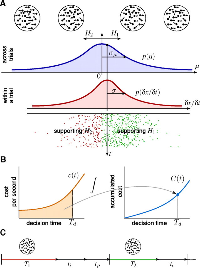
Direction discrimination task used to study perceptual decision making. A decision maker needs to decide whether the net direction of a random-dot stimulus is toward to the left or the right. A, Task trial and difficulty. At the beginning of each trial, μ is sampled from a Gaussian (blue curve). H₁ or H₂ are the correct choice if μ ≥ 0 or μ < 0, respectively. The magnitude |μ| is the evidence strength, which determines the difficulty of the trial. In the random-dot kinematogram, the sign of μ specifies the direction of motion, and its magnitude |μ| is proportional to the probability of each of the dots to move in the target direction. Within a trial, the distribution that the momentary evidence δx is sampled from (red curve), is centered on μ. Samples <0 (in red) and ≥0 (in green) support H₂ and H₁, respectively. B, Cost per second and accumulated cost. The left graph shows an example cost function c(t) that is initially constant and then rises over time. The right graph shows the accumulated cost C(t), which is the area underneath the cost function c(t). The decision maker has to pay a total cost of C(T_d), as shown in the right graph, for decisions made at time T_d. This cost corresponds to the shaded area in the left graph. C, Enumeration of total time. In the first of the two shown consecutive trials, an incorrect decision after T₁ seconds is followed by the intertrial interval t_i and some penalty time t_p. In the second trial, the decision after T₂ seconds is correct and is so only followed by the intertrial interval t_i.

The decision maker receives reward R_ij for choosing H_i when H_j is correct. Here, rewards can be positive or negative, allowing, for instance, for negative reinforcement when subjects pick the wrong hypothesis, that is, when i is different from j. Additionally, we assume the accumulation of evidence to come at a cost (internal to the decision maker), given by the cost function c(t). This cost is momentary, such that the total cost for accumulating evidence if a decision is made at decision time T_d after stimulus onset is C(T_d) = ∫₀^T_dc(t)dt (see Fig. 1B). Each trial ends after T_t seconds and is followed by the intertrial interval t_i and an optional penalty time t_p for wrong decisions (see Fig. 1C). We assume that decision makers aim at maximizing their reward rate, given by the following:

where the averages are over choices, decision times, and randomizations of t_i and t_p. We differentiate between fixed-duration tasks and reaction time tasks. In fixed-duration tasks, we assume T_t to be fixed by the experimenter and to be large when compared with T_d, and t_p = 0. This makes the denominator of Equation 1 constant with respect to the subject's behavior, such that maximizing the reward rate ρ becomes equal to maximizing the expected net reward 〈R〉 − 〈C(T_d)〉 for a single trial. In contrast, in reaction time tasks, we need to consider the whole sequence of trials when maximizing ρ because the denominator depends on the subject's reaction time through T_t, which, in turn, influences the ratio (provided that T_t is not too short compared with the intertrial interval and penalty time).

Optimal behavior for fixed-duration tasks.

We applied dynamic programming (Bellman, 1957; Bertsekas, 1995; Sutton and Barto, 1998) to derive the optimal strategy for repeated trials in fixed-duration tasks. As above, we present the technical details here and provide additional intuition in Results. At each point in time after stimulus onset, the decision maker can either accumulate more evidence, or choose either H₁ or H₂. As known from dynamic programming, the behavior that maximizes the expected net reward 〈R〉 − 〈C(t_d)〉 can be found by computing the “expected return” V(g,t). This quantity is the sum of all expected costs and rewards from time t after stimulus onset onwards, given belief g at time t, and assuming optimal behavior thereafter (that is, featuring behavior that maximizes the expected net reward). Since g is by definition the belief that H₁ is correct, this expected return is gR₁₁ + (1 − g)R₁₂ [or (1 − g)R₂₂ + gR₂₁] for choosing H₁ (or H₂) immediately, while collecting evidence for another δt seconds promises the expected return 〈V(g(t + δt),t + δt) | g,t〉_{g(t + δt)} but comes at cost c(t)δt. The expectation of the future expected return is over the belief p(g(t + δt) | g(t),t) that the decision maker expects to have at t + δt, given that she holds belief g(t) at time t. This density over future beliefs depends on the prior p(μ). Performing at each point in time the action (choose H₁/H₂ or gather more evidence) that maximizes the expected return results in Bellman's equation for fixed-duration tasks as follows:

For any fixed t, the max{.,.,.} operator in the above expression partitions the belief space {g} into three areas that determine for which beliefs accumulating more evidence is preferable to deciding immediately. For symmetric problems [when R₁₁ = R₂₂, R₁₂ = R₂₁, ∀μ: p(μ) = p(−μ)], this partition is symmetric around ½. Over time, this results in two time-dependent boundaries, g_θ(t) and 1 − g_θ(t), between which the decision maker ought to accumulate more evidence [Fig. 2 illustrates this concept; Fig. 3 provides examples for g_θ(t)]. When a boundary is reached, the decision maker should decide in favor of the hypothesis associated with that boundary. The boundary shape is determined by the solution to Equation 2, which we find numerically by backward induction, as shown below.

Figure 2.

The optimal behavior by dynamic programming, and diffusion model implementation. A, Finding the optimal behavior requires trading off the expected reward for immediate decisions with the cost and expected higher reward for later decisions. Assuming a fixed time t after stimulus onset, a reward of 1 for correct decision and 0 for incorrect decisions, the figure shows the total expected future costs and rewards [that is, the expected return V(g,t)] from time t onward, for different beliefs g and actions of the decision maker. The green line represents the expected reward, max{g,1 − g}, for deciding immediately and corresponds to the belief that H₁ (right half of graph) or H₂ (left half of graph) are the correct decision. Instead, if the decision maker accumulates more evidence, her expected return (that is, confidence), 〈V(g̃, t + δt) | g, t〉_g̃ taking future rewards and costs into account, will increase (red line). However, accumulating more evidence also comes at an immediate cost of c(t)δt, reducing its expected return (orange line). The optimal strategy is to choose the action that maximizes the expected return, such that the decision maker ought to accumulate more evidence as long as the associated expected return (orange line) dominates that of the expected return for making decisions immediately (green line). This partitions the belief space into three parts: as long as the decision maker's belief is between 1 − g_θ(t) and g_θ(t) (orange line above green line), the decision maker accumulates more evidence. Otherwise (green line above orange line), H₁ is chosen if g ≥ g_θ(t), and H₂ if g ≤ 1 − g_θ(t). g_θ(t) changes over time as (1) the cost function might change over time, and (2) the expected return for accumulating more evidence depends on how the decision maker expects to trade off costs and reward in the future, for times after t. B, The optimal behavior can be implemented by a diffusion model with time-varying boundaries {−θ(t),θ(t)} in particle space, corresponding to the bounds {1 − g_θ(t), g_θ(t)} in belief space. The particle location x(t) is determined by integration of momentary evidence δx. As soon as the particle hits the upper bound θ(t) [lower bound, −θ(t)], H₁ (H₂) is chosen. Five particle trajectories with fixed drift μ are shown, three of which lead to the—for this drift correct—choice of H₁ (shown in yellow).

Figure 3.

Optimal behavior in fixed-duration and reaction time tasks. All panels show the belief at the decision boundary, g_θ(t), which defines the threshold in belief and time at which a decision is to be made to perform optimally. This threshold depends on various parameters, such as the cost function, the task difficulty, and the intertrial interval in reaction time tasks. Only the upper bound g_θ(t) is shown as the lower bound 1 − g_θ(t) is mirror-symmetric to it around belief ½. A, Fixed-duration single-evidence strength trials, μ ϵ {½,−½}, constant cost c(t) over time, for different magnitudes of that cost. B, Fixed-duration trials with variable evidence strength, μ∼N(0,σ_μ²), constant cost c(t) = ½, for different task difficulties 1/σ_μ² (the harder the task, the larger 1/σ_μ²). C, Reaction time task with different intertrial intervals t_i, σ_μ² = 16, c(t) = ½. The dashed green curve corresponds to t_i → ∞ and is equivalent to the solid green curve in B. D, Reaction time task with increasing cost function c(t) = at [C(t) is quadratic in t], t_i = 1, σ_μ² = 16, a specified in legend. In all panels, t_p = 0, reward 1 for correct choices and no punishment for wrong choices.

Optimal behavior for reaction time tasks.

We solved for the optimal behavior in reaction time tasks by maximizing the whole reward rate, Equation 1, rather than just its numerator. This reward rate depends not only on the expected net reward in the current trial, but through the expected trial time 〈T_t〉 and the penalty time 〈t_p〉 also on the behavior in all future trials. Thus, if we were to maximize the expected return V(g,t) to determine the optimal behavior, we would need to formulate it for the whole sequence of trials (with t = 0 now indicating the stimulus onset of the first trial instead of that of each of the trials). However, this calculation is impractical for realistic numbers of trials. We therefore exploited a strategy used in “average reward reinforcement learning” (Mahadevan, 1996), which effectively penalizes the passage of time. Instead of maximizing V(g,t), we use the “average-adjusted expected return” Ṽ(g, t) = V(g, t) − ρt, which is the standard expected return minus ρt for the passage of some time t, where ρ is the reward rate (for now assumed to be known). The strategy is based on the following idea. At the beginning of each trial, the decision maker expects to receive the reward rate ρ times the time until the beginning of the next trial. This amount equals the expected return V(½, 0) for a single trial, as above. Therefore, removing this amount from the expected return causes the average-adjusted expected return to become the same at the beginning of each trial. This adjustment allows us to treat all trials as if they were the same, single trial.

As for fixed-duration tasks, the optimal behavior is determined by, in any state, choosing the action that maximizes the average-adjusted expected return. Since the probability that option 1 is the correct one is, by definition, the belief g, choosing H₁ would result in the immediate expected reward gR₁₁ + (1 − g)R₁₂. The expected intertrial interval is 〈t_i〉 + (1 − g)t̄_p after which the average-adjusted expected return is Ṽ(½, 0), with t_i denoting the standard intertrial interval, t_p the penalty time for wrong choices, and where t̄_p = 〈t_p| wrong choice〉 (that is, assuming a penalty time that is randomized, has mean t̄_p, and only occurs in trials where the wrong choice has been made). At the beginning of each trial, at t = 0, the belief held by the subject is g = ½, such that the average-adjusted expected return at this point is Ṽ(½, 0). Thus, the average-adjusted expected return for choosing H₁ is gR₁₁ + (1 − g)R₁₂ − (〈t_i〉 + (1 − g)t̄_p)ρ + Ṽ(½, 0). Analogously, the average-adjusted expected return for choosing H₂ is (1 − g)R₂₂ + gR₂₁ − (〈t_i〉 + gt̄_p)ρ + Ṽ(½, 0). When collecting further evidence, one needs to only wait δt, such that average-adjusted expected return for this action is 〈Ṽ(g(t + δt),t + δt) | g, t〉_g(t+δt) − c(t)δt − ρδt. As we always ought to choose the action that maximizes this return, the expression for Ṽ(g, t) is the maximum of the returns for the three available actions. This expression turns out to be invariant with respect to the resulting behavior under the addition of a constant (that is, replacing all occurrences of Ṽ(g, t) by Ṽ(g, t) + K, where K is an arbitrary constant, results in the same behavior). We remove this degree of freedom and at the same time simplify the equation by choosing the average-adjusted expected return at the beginning of each trial to be Ṽ(½, 0) = 0. This results in Bellman's equation for reaction time tasks to be the following:

The optimal behavior can be determined from the solution to this equation (see Results) (see Fig. 2A). Additionally, it allows us to find the reward rate ρ: Bellman's equation is only consistent if—according to our previous choice—Ṽ(½, 0) = 0. Therefore, we can initially guess some ρ, resulting in some nonzero Ṽ(½, 0), and then improve the estimate of ρ iteratively by root finding until Ṽ(½, 0) = 0.

Optimal behavior with minimum reward time.

The experimental protocol used to collect the behavioral data from monkeys differed from a pure reaction time task because of implementation of a “minimum reward time” t_r. When the monkeys decided before t_r, the delivery of the reward was delayed until t_r, whereas decisions after t_r resulted in immediate reward. Since the intertrial interval began after the reward was administered, the minimum reward time effectively extends the time the decision maker has to wait until the next stimulus onset on some trials. This is captured by a decision time-dependent effective intertrial interval, given by t_i,eff(t) = 〈t_i〉 + max{0,t_r − t}. If the decision is made before passage of the minimum reward time such that t_r > t, then the effective intertrial interval is t_i,eff(t) = 〈t_i〉 + t_r − t, which is larger than the standard intertrial interval, t_i. Otherwise, if t ≥ t_r, the effective intertrial interval equals the standard intertrial interval, that is t_i,eff(t) = 〈t_i〉. This change allows us to apply the Bellman equation for reaction time tasks to the monkey experiments. We simply replace 〈t_i〉 by t_i,eff(t) in Equation 3.

Solving Bellman's equation.

Finding the optimal behavior in either task type requires solving the respective Bellman equation. To do so, we assume all task contingencies [that is, prior p(μ), the cost function c(t), and task timings t_i and t_p] to be known, such that V(g,t) for g ϵ (0,1) and t ϵ [0,…] remains to be computed. As no analytical solution is known for the general case we treat here, we solve the equation numerically by discretizing both belief and time (Brockwell and Kadane, 2003). We discretized g into 500 equally sized steps while skipping g = 0 and g = 1 to avoid singularities in p(g(t + δt) | g(t),t). The step size in time δt cannot be made too small, as a smaller δt requires a finer discretization in g to represent p(g(t + δt) | g(t),t) adequately. We have chosen δt = 5 ms for all computations presented in Results, but smaller values (for example, δt = 2 ms, as applied to some test cases) gave identical results.

For fixed-duration tasks, the discretized version of V(g,t) can be solved by backward induction: if we know V(g,T) for some T and all g, we can compute V(g,T − δt) by use of Equation 2. Consecutively, this allows us to compute V(g,T − 2δt) using the same equation, and in this way evaluate V(g,t) iteratively for all t = T − δt, T − 2δt,…, 0 by working backward in time. The only problem that remains is to find a T for which we know the initial condition V(g,T). We approach this problem by assuming that, after a very long time T, the decision maker is guaranteed to commit to a decision. Thus, at this time, the only available options are to choose either H₁ or H₂. As a consequence, the expected return at time T is V(g,T) = max{gR₁₁ + (1 − g)R₁₂, (1 − g)R₂₂ + gR₂₁}, which equals Equation 2 if one removes the possibility of accumulating further evidence. This V(g,T) can be evaluated regardless of V(g,T + δt) and is thus known. T was chosen to be five times the time frame of interest. For example, if all decisions occurred within 2 s after stimulus onset, we used T = 10 s. No significant change in V(g,t) (within the time of interest) was found by setting T to larger values.

We find the average-adjusted expected return Ṽ(g, t) similarly to V(g,t) by discretization and backwards induction on Eq. (3). However, as ρ is unknown, we need to initially assume its value, compute Ṽ(½, 0), and then adjust ρ iteratively by root finding (Ṽ(½, 0) changes monotonically with ρ) until Ṽ(½, 0) = 0.

Belief for Gaussian priors.

The data we analyzed used a set of discrete motion strengths, and we used a prior on μ reflecting this structure in our model fits (see next section). Nonetheless, we provide here the expression for belief resulting from assuming a Gaussian prior p(μ) = N(μ | 0,σ_μ²) for evidence strength over trials, as this prior leads to more intuitive mathematical expressions. The prior assumes that the evidence strength |μ| is most likely small but occasionally can take larger values. We find the posterior μ given all evidence δx_0…t up to time t by Bayes' rule, p(μ | δx_0…t) ∝ p(μ)∏_n N(δx_n | μδt,δt), resulting in

where we have used the sufficient statistics t = Σ_nδt and x(t) = Σ_nδx_n. With the above, the belief g(t) ≡ p(μ ≥ 0 | δx_0…t) is given by the following:

where Φ ( · ) is the standard normal cumulative function. Thus, the belief is g(t) > ½ if x(t) > 0, g(t) < ½ if x(t) < 0, and g(t) = ½ if x(t) = 0. The mapping between x(t) and g(t) given t is one-to-one and is inverted by the following:

where Φ⁻¹ ( · ) is the inverse of a standard normal cumulative function.

Belief for general symmetric priors.

Assume that the evidence strength can take one of M specific non-negative values {μ₁,…,μ_M}, at least one of which is strictly positive, and some evidence strength μ_m is chosen at the beginning of each trial with probability p_m, satisfying Σ_mp_m = 1. Let the prior p(μ) be given by p(μ = μ_m) = p(μ = −μ_m) = p_m/2 for all m = 1,…, M. In some cases, one might want to introduce a point mass at μ_m = 0. To share such a mass equally between μ < 0 and μ > 0, we handle this case by transforming this single point mass into equally weighted point masses p(μ = ϵ) = p(μ = −ϵ) = p_m/2 for some arbitrarily small ϵ. The resulting prior is symmetric, that is, p(μ) = p(−μ) for all μ, and general, as it can describe all discrete probability distributions that are symmetric around 0. It can be easily extended to also include continuous distributions.

With this prior, the posterior of μ having the value μ_m given all evidence δx_0…t up to time t is as before found by Bayes' rule, and results in the following:

The belief at time t is defined as g(t) ≡ p(μ ≥ 0 | δx_0…t) and is therefore given by the following:

It has the same general properties as for a Gaussian prior and is strictly increasing with x(t), such that the mapping between g(t) and x(t) is one-to-one and can be efficiently inverted by root finding.

Accumulating evidence in the presence of a bound.

The mapping between g(t) and x(t) in Equations 5 and 8 was derived without a bound in particle space {x}. Here, we show that it also holds in the presence of a bound (Moreno-Bote, 2010). This property is critical because it underlies the assertion that the diffusion model with time-varying boundaries performs optimally (see Results). Intuitively, the crucial feature of the mapping between g(t) and x(t) is that g(t) does not depend on the whole trajectory of the particle up to time t but only on its current location x(t). As such, it is valid for all possible particle trajectories that end in this location. If we now introduce some arbitrary bounds in particle space and remove all particle trajectories that have crossed the bound before t, there are potentially fewer trajectories that lead to x(t), but the endpoint of these leftover trajectories remains unchanged and so does their mapping to g(t). Therefore, this mapping is valid even in the presence of arbitrary bounds in particle space.

More formally, assume two time-varying bounds, upper bound θ₁(t) and lower bound θ₂(t), with θ₂(0) < 0 < θ₁(0) and θ₁(t) ≥ θ₂(t) for all t > 0. Fix some time t of interest, and let x̄ denote a particle trajectory with location x̄(s) for s ≤ t. Also, let Ω(x(t)) = {x̄:θ₂(s) < x̄(s) < θ₁(s) ∀ s < t,x̄(t) = x(t)} denote the set of all particle trajectories that have location x(t) at t and did not reach either bound before that. The posterior of μ given only the trajectory endpoint is thus given by the following:

where $\underset{\mu }{\propto }$ denotes a proportionality with respect to μ. The path integral sums over all trajectories that have not reached the bound before t. Considering a single of these trajectories, it can be split into small steps δx̄(t) = x̄(t + δt) − x̄(t) distributed as N(δx̄(t) | μδt,δt), such that its probability is given by the following:

where $x\left(t\right)={\Sigma }_{n=0}^{\raisebox{1ex}{$t$}\!\left/ \!\raisebox{-1ex}{$\delta t$}\right.}\delta \overline{x}\left(n\delta t\right)$ and $t={\Sigma }_{n=0}^{\raisebox{1ex}{$t$}\!\left/ \!\raisebox{-1ex}{$\delta t$}\right.}$ was used, and D(x̄) is a function of the trajectory that captures all terms that are independent of μ. This already clearly shows that, as a likelihood of μ, p(x | μ) is proportional to some function of x(t) and t, with only its proportionality factor being dependent on the full trajectory. Using this expression in the posterior of μ results in the following:

Therefore, the posterior of μ does not depend on Ω(x(t)) and is thus independent of the presence and shape of boundaries. As the belief g(t) is fully defined by the posterior of μ, it shares the same properties.

Belief transition densities.

Solving Bellman's equation to find the optimal behavior requires us to evaluate 〈V(g(t + δt),t + δt) | g,t〉_{g(t + δt)}, which is a function of V(g(t + δt),t + δt) and p(g(t + δt) | g(t),t). Here, we derive an expression for p(g(t + δt) | g(t),t) for small δt, for a Gaussian prior, and for a general symmetric prior on μ.

In both cases, the procedure is the same: using the one-to-one mapping between g and x, we get p(g(t + δt) | g(t),t) from the transformation p(g(t + δt) | g(t),t)dg(t + δt) = p(x(t + δt) | x(t),t)dx(t + δt). The right-hand side of this expression describes a density over future particle locations x(t + δt) after some time δt given the current particle location x(t). The latter allows us to infer about the value of μ from which we can deduce the future location by p(x(t + δt) | x(t),t) = ∫p(x(t + δt) | μ,x(t),t)p(μ | x(t),t)dμ. Given μ, the future particle location is p(x(t + δt) | μ,x(t),t) = N(x(t + δt) | x(t) + μδt,δt) due to the standard diffusion from known location x. This expression ignores the presence of a bound during the brief time interval δt. Therefore, our approach is valid in the limit in which δt goes to zero. Practically, a sufficiently small δt (as used when solving Bellman's equation) will cause the error due to ignoring the bound to be negligible. Note that p(μ | x(t),t) depends on the prior p(μ), and so does dx(t + δt)/dg(t + δt).

If p(μ) is Gaussian, p(μ) = N(μ | 0,σ_μ²), the mapping between g(t) and x(t) is given by Equations 5 and 6. For the mapping between g(t + δt) and x(t + δt), t in these equations has to be replaced by t + δt. The posterior of μ given x(t) and t is given by Equation 4, such that the particle transition density results in p(x(t + δt) | x(t),t) = N(x(t + δt) | x(t)(1 + δt_eff),δt(1 + δt_eff)), where we have defined δt_eff = δt/(1 + ${\raisebox{1ex}{$1$}\!\left/ \!\raisebox{-1ex}{$\sigma $}\right.}_{\mu }^2$). As g(t + δt) is the cumulative function of x(t + δt), its derivative with respect to x(t + δt) is the Gaussian dg(t + δt)/dx(t + δt) = N(x(t + δt) | 0,t + δt + ${\raisebox{1ex}{$1$}\!\left/ \!\raisebox{-1ex}{$\sigma $}\right.}_{\mu }^2$). Combining all of the above, replacing all x(t) and x(t + δt) with their mapping to g(t) and g(t + δt) result, after some simplification, in the following:

If p(μ) is the previously introduced discrete symmetric prior, we have the mapping between g(t) and x(t) given by Equation 8. To simplify notation, define

such that the mapping between g(t) and x(t) can be written as g(t) = Σ_ma_m/Σ_n(a_n + b_n) = f_t(x(t)). Even though f_t(x(t)) is not analytically invertible, it is strictly increasing with x(t) and can therefore be easily inverted by root finding. The same mapping is established between g(t + δt) and x(t + δt) by replacing all a and b by ã and b̃. Using the same notation, the posterior of μ given x(t) and t (Eq. 7) is p(μ = μ_m | x(t),t) = a_m/Σ_n(a_n + b_n) and p(μ = − μ_m | x(t),t) = b_m/Σ_n(a_n + b_n), such that the particle transition density after some simplification is as follows:

Based on the mapping between g(t + δt) and x(t + δt), we also find the following:

Combining all of the above results in the following belief transition density:

Belief equals choice accuracy.

To compute the cost function that corresponds to some observed behavior, we need to access the decision maker's belief at decision time. We do so by establishing (shown below) that, for the family of diffusion models with time-varying boundaries that we use, the decision maker's belief at decision time equals the probability of making the correct choice (as observed by the experimenter) at that time. Note that showing this for the family of diffusion models does not necessarily imply that the belief held by the actual decision maker equals her choice accuracy, especially if the integration of evidence model of the decision maker does not correspond to a diffusion model or she has an incorrect model of the world. However, we will assume that subjects follow such optimal diffusion models, and therefore we infer the decision maker's belief of being correct at some time by counting which fraction of choices performed at this time lead to a correct decision.

The diffusion model is bounded by the time-varying symmetric functions −θ(t), and θ(t), and a decision is made if the diffusing particle x reaches either boundary, that is x = ±θ(t). If μ ≥ 0, then the boundary that leads to the correct decision is x = θ(t). Therefore, the choice accuracy, which is the probability of a decision being correct given that a decision was made, is p(x = θ(t) | x = ±θ(t),t,μ ≥ 0). However, the subject's belief at the point this decision was made is g_θ(t) ≡ p(μ ≥ 0 | x = θ(t),t). Choice accuracy equals belief if these two probabilities are identical. We show this to be the case, provided that (1) the prior on μ is symmetric, that is, p(μ) = p(−μ), for all μ, and that (2) the process features mirror symmetry, that is, p(x = θ(t) | μ < 0,t) = p(x = −θ(t) | μ ≥ 0,t). It is easy show that both conditions hold in our case. Applying Bayes' theorem to the decision maker's belief, we get the following:

For the second equality, we have used the symmetry of the prior and the mirror symmetry of the process to modify the second term in the denominator. The third equality follows from the definition of the conditional probabilities.

Predicting belief over time per evidence strength.

Given knowledge of the prior p(μ) and how the bound θ(t) in a diffusion model (DM) (see Results) (see Fig. 2B) changes over time, we can predict how the change in choice accuracy with time depends on the evidence strength. This does not contradict that the belief g_θ(t) at decision time does not depend on the evidence strength. Rather, we are adding information (the evidence strength) that is not available to the decision maker, and averaging over this information makes the belief independent again, that is, the following:

Nonetheless, we (who have access to the evidence strength) use it to test the validity of the proposed DM by investigating if the change in observed choice accuracy follows the prediction (see Fig. 10B).

Figure 10.

Data and model prediction for change of choice accuracy over time per coherence. Smoothing and shaded areas are as in Figure 4. The fits are based on computing the choice accuracy for a given evidence strength (see Materials and Methods), based on the fitted DM bounds (Fig. 5) mapped from decision times to reaction times. These fits confirm that the choice accuracy for all evidence strengths are well captured by a single time-varying DM bound that does not depend on this evidence strength. This, in turn, supports the hypothesis that the decision threshold that the observed decisions are based on depends solely on belief and time.

We first find the belief at bound given that the evidence strength, |μ| = μ₀, is known, but the sign of μ is unknown, by applying Equation 8 with M = 1, p₁ = 1, and μ₁ = μ₀ (that is, a prior on μ with two point masses located at ±μ₀) and replacing x(t) with θ(t) in the resulting expression. This belief would be the one the decision maker holds at the time of the decision, given that she were informed about the evidence strength |μ₀|. Furthermore, our previously derived result that belief equals choice accuracy does only depend on the symmetry but not the exact form of the prior and thus also holds in this case. This leads to the final expression for choice accuracy given evidence strength to be given by the following:

This is a generalization of the known expression for first-passage probabilities of DM (Cox and Miller, 1965) to time-varying boundaries.

Computing the cost function from behavior.

We compute the cost function from observed behavior by reversing the dynamic programming procedure used to find the optimal behavior for a given cost function. We assume that the belief g_θ(t) at the decision time t corresponds to the fraction of correct choices at this time (see above), such that this belief can be inferred from the observation of choice behavior. This is only valid for reaction time tasks at which we have access to both choice and decision time. In fixed-duration trials, the decision maker can commit to a decision before the end of the trial, which invalidates the approach used here. We only consider cases with symmetric reward (R₁₁ = R₂₂, and R₁₂ = R₂₁), but the same procedure can be adapted to tasks in which this is not the case.

Assuming for now knowledge of the reward rate ρ, we find c(t) from g_θ(t) as follows: g_θ(t) is by definition the belief at which the expected return of deciding immediately equals that of accumulating more evidence and deciding later. If we apply this equality using the different terms in Equation 3 and solve for c(t), we find the following:

For tasks with a minimum reward time, 〈t_i〉 is again replaced by t_i,eff(t). Thus, given that Ṽ(g, t + δt) and g_θ(t) are known, the cost c(t) can be computed. Additionally, as c(t) is now known, it can be used to find Ṽ(g, t) (as before, with some adequate discretization of g and t), which in turn can be used to find c(t − δt), and so on. This allows us to compute all c(t) and Ṽ(g, t) for t < T by backward induction, starting at some known Ṽ(g, T). We find the latter by assuming that the decision maker is guaranteed to never continue accumulating more evidence after the last observed decision time T, such that Ṽ(g, T) becomes the (known) expected return for deciding immediately.

The reward rate ρ is found self-consistently by using the condition Ṽ(½, 0) = 0. If we initially assume some ρ (we usually start at ρ = 0), Ṽ(½, 0) is computed by the above procedure, and ρ is adjusted iteratively by root finding until Ṽ(½, 0) = 0.

Modeling behavior.

To compute the cost function from the belief at decision time, g_θ(t), we can invoke the equality between belief and choice accuracy (see above), and thus need to know the subject's decision accuracy at any point in time after stimulus onset.

We assume the measured reaction time to consist of the decision time (described by the DM) as well as the nondecision time. The latter is a random variable that is composed of the time from stimulus onset to the point at which the subject starts accumulating evidence, and the motor time that it takes the subject to initiate the adequate behavior after a decision has been made. This nondecision time needs to be discounted from the reaction time to find the decision time for each observed trial. Additionally, the behavior data is confounded with lapse trials, in which the behavior is assumed random, independent of the stimulus. This makes determining the decision accuracy more complicated than simply binning time and plotting the percentage of correct choices per bin. Instead, we use a parametric generative-model approach that explicitly models both the nondecision time and the lapse trials. This model is described next, followed by how we find its parameter posterior by Bayesian inference. After that, we describe how this posterior is used to predict behavior, belief over time, and how the latter is used to compute the cost function.

Let t_n be the reaction time in the nth of N observed trials (consisting of the decision time s_n and some nondecision time t_n − s_n), and let x_n be the corresponding decision (0/1 for correct/incorrect choices). In each trial, the experimenter controls some independent variable c_n that, similar to previous DMs for the random-dot kinetogram, determines the evidence strength by |μ_n| = kc_n, where k is a model parameter. The decision time s_n and choice x_n in nonlapse trials are assumed to be describable by a DM with time-changing boundaries, θ(s) and −θ(s), given by a weighted sum of cosine basis functions as follows:

where the cos(a) function returns the cosine of a for −π ≤ a ≤ π, and 0 otherwise, and T_max is the 95th percentile of the subject's distribution of observed reaction times. The parameter ν controls the spacing of the basis functions in s, and {w₁,…,w_B} are their weights. Given this bound and a certain evidence strength, we numerically compute the first-passage time densities as the solution of a Volterra integral equation of the second kind (Smith, 2000), and denoted h₁(s_n;c_n,γ) for bound θ(s) (correct decisions), and h₀(s_n;c_n,γ) for bound −θ(s) (incorrect decisions), with γ being the set of all model parameters. Thus, h_xn(s_n;c_n,γ) denotes the probability density of making choice x_n at decision time s_n in a trial with evidence strength kc_n.

The nondecision time t_n − s_n is modeled by a half-Gaussian p(t_n − s_n | γ) = 2N(t_n − s_n | μ_nd,σ_nd²) for t_n − s_n ≥ μ_nd, with minimal nondecision time μ_nd and scale σ_nd (Vanderkerckhove et al., 2008). The decision time itself is not inferred explicitly, as the first passage-time can be expressed in terms of the reaction time by numerically marginalizing out the decision time, h̃_xn(t_n;c_n,γ) = ∫₀^∞p(t_n | s_n,γ)h̃_xn(s_n;c_n,γ)ds_n. Therefore, the likelihood for a nonlapse trial n with reaction time t_n and decision x_n is given by h̃_xn(t_n;c_n,γ). In lapse trials, the decision is assumed to be random, and the reaction time uniform over the range [T_min,T_max], such that the likelihood of a lapse trial is 1/(2(T_max − T_min)). T_min and T_max are the smallest and largest observed reaction time, respectively, discarding the slowest 5% of trials. We assume that any trial is a lapse trial with probability p_l, such that the full likelihood of trial n is give by the following mixture:

This completes the specification of the generative model, with its B + 5 parameters γ = {k,ν,w₁,…,w_B,μ_nd,σ_nd,p_l}. The model parameters do not include the prior p(μ), as we assumed the subjects (which are highly trained) to have learned either p(μ) or the correct prior over the coherences, c, which leads to p(μ) by |μ| = kc.

The aim when fitting the model is to find the posterior p(γ | X,T,C) where X = {x₁,…,x_N} is the set of observed decisions, T = {t₁,…,t_N} is the set of observed reaction times, and C = {c₁,…,c_N} is the set of independent variables (coherences, in this case) controlled by the experimenter. We assume the priors over all parameters to be uniform over the ranges k ϵ [0.1,100], ν ϵ [0.1,1], w_b ϵ [0,6], μ_nd ϵ [0,T_max], σ_nd ϵ [0,T_max], and p_l ϵ [0,0.5]. We draw samples from the posterior (Lee et al., 2007), using the Markov Chain Monte Carlo method known as slice sampling (Neal, 2003), which only requires us to know the log-posterior up to a normalization constant. The number of basis functions is chosen to be B = 10, and the decision time distributions h̃_xn (·) are computed in steps of 1 ms. We have drawn a total of 200,000 samples (400,000 for the human subjects) from the posterior, but discarded the first 20,000 burn-in samples. All predictions are based on 500 samples drawn randomly from the leftover posterior samples.

Despite the high number of model parameters, we avoid overfitting by marginalizing over the parameter posterior. All model predictions are based on Monte Carlo approximation with 500 samples {γ⁽¹⁾,…,γ⁽⁵⁰⁰⁾} approximating the jth moment of some function f(γ) by 〈f(γ)〉^j ≈ 1/500Σ_if(γ⁽ⁱ⁾)^j. For each of the samples, γ⁽ⁱ⁾, the mean reaction times per coherence, as well as the probability correct, are computed numerically from h̃₀(·) and h̃₁(·). The belief g_θ(t) over time is found by using Equation 8. The cost function is computed from this belief as described above.

Data sets and analysis.

We compute the cost function based on data from two behaving monkeys and six behaving humans performing a reaction time, motion discrimination task. The task is described in Results and further details on animal and human design are in the studies by Roitman and Shadlen (2002) and Palmer et al. (2005) (Experiment 1), respectively. For both data sets, each trial is described by a reaction time (the time from stimulus onset to saccade onset), the subjects' decision, and the actual motion direction and strength (coherence of the visual stimulus, out of {0, 3.2, 6.4, 12.8, 25.6, 51.2%}).

The monkey dataset consists of 2615 trials for monkey B and 3534 trials for monkey N (Table 1). Overall, 95% of decisions are made in <1030 ms (1134 ms) from stimulus onset for monkey B (monkey N), and most figures only show data and fits up to these reaction times. Computing the cost function requires additional information about the timing between consecutive trials, such as minimum reward delay (800 ms for monkey B; 1200 ms for monkey N), the average time the monkeys required to fixate the fixation point before a new trial was initiated (1462 ms for monkey B; 1242 ms for monkey N), the average delay duration between fixation and appearance of the saccade targets (861 ms for monkey B; 652 ms for monkey N), and the average delay from target onset to stimulus onset (700 ms for both monkeys). For all saccades that are performed after the minimum reward time, reward is delayed an average of 149 ms for monkey B, and 116 ms for monkey N. Given that this delay also occurs in trials in which the reaction time is smaller than the minimum reward time, it shortens the effective minimum reward time to 651 ms for monkey B and 1084 ms for monkey N. Overall, the effective average intertrial interval, being the time from saccade to stimulus onset of the next trial, becomes 2311 ms for monkey B and 2058 ms for monkey N. The final intertrial interval used to compute the cost function was given by these values, and additionally by the average nondecision time (as determined by the model fits), as the latter does contribute to the decision process itself.

Table 1.

Fit quality per subject

	Trials	Coefficient of determination, R2			AIC	AICconst	KS
		Chron	Psych	Avg
Palmer et al. (2005)
AH	554	0.948	0.974	0.961	−167.85 (±4.16)	33.90	1 (p < 0.01)
EH	560	0.952	0.944	0.948	245.11 (±3.71)	347.41	1 (p < 0.05)
JD	567	0.897	0.974	0.936	−558.39 (±57.68)	516.36	3 (p < 0.01)
JP	555	0.976	0.998	0.987	−330.01 (±5.28)	2754.84	2 (p < 0.05)
MK	573	0.973	0.993	0.983	−504.24 (±4.60)	2041.61	2 (p < 0.01)
MM	564	0.928	0.978	0.953	−262.25 (±3.65)	107.83	0
Avg	562.2 (±3.3)	0.946 (±0.013)	0.977 (±0.008)	0.961 (±0.009)
Roitman and Shadlen (2002)
B	2615	0.985	0.989	0.987	−809.16 (±18.99)	26,436.32	0
N	3534	0.983	0.991	0.987	620.34 (±33.69)	48,005.64	3 (p < 0.05)

The table shows, for each subject, the number of trials that were fitted; the coefficient of determination (R²) for the chronometric function (Chron), the psychometric function (Psych), and averaged over both (Avg); the goodness of fit of our model according to the AIC (smaller is better), and the comparison goodness of fit of a diffusion model with constant bound (AICconst); the number of conditions (out of 12) for which the Kolmogorov–Smirnov test revealed a statistical significance between the reaction time distribution featured by the subject and that predicted by the model, together with the level of significance (KS). For the human dataset, we also provide the mean across subjects (±1 SEM) for the number of trials and the coefficient of determination. The AIC measure for our model is computed separately for 500 posterior samples, and here we provide mean ± 1 SD.

The human dataset consists of behavioral data collected from six highly practiced subjects (AH, EH, JD, JP, MK, and MM; three females), with an average of 562.2 ± 3.3 trials per subject (Table 1). The task sequence resembled the one used in the neurophysiology experiments. The random-dot motion was presented at a random interval after the subject attained fixation (mean, 900 ms; minimum, 500 ms). The subject terminated a trial by breaking fixation and making a saccade to one of the choice targets, thereby marking the end of the trial, at which point the display was blank. Subjects received feedback for correct choices. The fixation point reappeared to begin the next trial 1.5 or 2 s after the choice saccade, for correct and error trials, respectively. We assume that it took the subjects 500 ms on average to acquire fixation of the centered disc (data not available). As for the monkeys, the individual subject's average nondecision time was added to the intertrial intervals when computing the cost function.

The human subjects received monetary reward that was independent of their performance. Thus, it was unclear whether they adjusted their speed/accuracy trade-off to maximize their number of correct decisions by unit time or, for example, put more emphasis on the correctness of their decisions. Despite this uncertainty, we analyzed their behavior as if their aim was to maximize their reward rate but we also assumed different levels of punishment for incorrect decisions, thus incorporating variation in weight given to correctness. Such variation did not affect our conclusions qualitatively. Our results are therefore robust to variations in the goals pursued by the subjects.

The data were modeled for each subject individually by sampling from the model parameter posterior. The human data were sufficiently well explained without the lapse model, which we disabled for this dataset by setting p_l = 0. For both datasets, we found a pointwise prior on the individual coherences used in the experiment to give a better fit than a Gaussian prior on μ. The model predicts full reaction time distributions for correct and incorrect decisions for each coherence, and a two-tailed one-sample Kolmogorov–Smirnov test was used for each of these distributions to test whether the observed behavior deviates significantly from these. To evaluate the quality of the psychometric and chronometric curves, we compute the coefficient of determination, R², by weighting each datum in proportion to the number of trials it represents. For the psychometric curve, the data are split by coherence, and for the chronometric curve, it is additionally split by correct/incorrect choices.

In addition to the coefficient of variation, we evaluated the fit quality using the Akaike information criterion (AIC), which takes into account the number of parameters in the model (Akaike, 1974). As the definition of the AIC relies on the model likelihood, we computed the AIC separately for all 500 posterior parameter samples. We report its mean and SD for each subject across all these samples. Furthermore, we compared our model to the fit of a standard DM with constant bounds by fitting the behavior of each subject separately, as described by Palmer et al. (2005). We then measured its fit quality by computing the AIC based on the likelihood of the full reaction time distributions as predicted by this DM. All quality-of-fit measures are reported in Table 1. The large variance in AIC across subjects for the DM with constant bounds stems from this DM assigning a very low likelihood to some trials, which leads to a very large AIC (that is, a poor fit) for some subjects. It might come as a surprised that the DM with constant bound provides poor fits for some subjects given previous reports that such DMs provide tight fits to subjects' performance. However, it is important to keep in mind that the previous studies reported that DMs with a constant bound can fit the accuracy and mean reaction time for correct trials (Palmer et al., 2005), but not necessarily the reaction time distributions or the mean reaction times on error trials (Ditterich, 2006b; Churchland et al., 2008).

The cost functions for both monkeys (see Fig. 7) and humans (see Fig. 9) were computed based on the fitted shape of the boundary of the diffusion model. To combine the cost function estimates for the different human subjects, we first shift each of them to feature a mean that is 0 at 100 ms. The shifted estimates are combined under the assumption that, at any point in time, they are noisy samples [mean μ_c,n(t) and SD σ_c,n(t) for subject n] of the “true” cost function. Based on these samples, the combined cost function has mean ${\mu }_c\left(t\right)=\Sigma n{\mu }_{c,n}{\left(t\right)}^{{\sigma }_c^2\left(t\right)}/{\sigma }_{c,n}^2\left(t\right)\text{and}\text{SD}{\sigma }_c\left(t\right)=1/\sqrt{\Sigma n{\raisebox{1ex}{$1$}\!\left/ \!\raisebox{-1ex}{$\sigma $}\right.}_{c,n}^2\left(t\right)}$ with the sums being over the six subjects, n = 1,…,6. The combined μ_c(t) and σ_c(t) are shown in Figure 9.

Figure 7.

Cost function for monkeys and representative human subject for different reward contingencies. The reward internal to the subjects is not accessible and thus a free parameter. For each subject, we compute the cost function for various settings of this free parameter (reward always 1 for correct decisions; punishment for incorrect decisions either 0, 1, or 2). The results do not qualitatively depend on the choice of these parameters. The estimated cost function c(t) itself is per second, such that the total cost for making a decision at time t is the area underneath the cost function up to time t. For the two monkeys, the gray dashed line represents the minimum reward time distribution. The minimum reward time relates to the reaction time of the decision maker. It is here mapped into the decision time by subtracting the nondecision time as estimated for each monkey separately. This estimate is a random variable, such that the minimum reward time also becomes a random variable in the decision time domain.

Figure 9.

Urgency signal depends solely on time and is independent of coherence. The urgency signal is the time-dependent change in activity that is shared by all belief-encoding neurons, independent of which aspect of the belief they encode. In combination with a constant bound on activity, this signal causes the effective bound on belief to collapse over time. The exact relationship between the bound collapse and the urgency signal depends on the encoding scheme. A, Here, we assume a simple encoding scheme, in which the neural activity, r₁(t) and r₂(t) of two perfectly anticorrelated neurons encodes the DM particle location x(t) by r₁(t) = r₀ + x(t) + u(t) and r₂ = r₀ − x(t) + u(t), with r₀ being a positive constant and u(t) being the urgency signal. A decision is made as soon as the activity of either neuron reaches a time-invariant threshold θ̃ > r₀. As shown in the bottom panel, a rising urgency signal speeds up the decisions (solid vs dashed trace). This is caused by the urgency signal effectively causing a collapse of the bounds {θ̃ − u(t), θ̃ + u(t)} acting on the diffusing particle x(t) = (r₁(t) − r₂(t))/2, as illustrated in the top panel. We emphasize that we are not committed to the particular DM-like encoding scheme. We used it for illustrative purposes only. Other schemes could be used but the relationship between the urgency signal and the collapse of the bound is less obvious. B, Average firing rate of neurons in the intraparietal cortex (LIP) of monkeys performing a dynamic random-dot display reaction time task (Churchland et al., 2008), for different coherences and for motion toward (T_in) and against (T_out) the response field of the neurons. The change of activity of these neurons seems to reflect the evidence accumulation process, which terminates whenever the activity of one population (for example, supporting H₁) reaches a threshold whose value is independent of coherence and time. This suggests an encoding scheme with a constant decision bound and an urgency signal that accelerates the race of the neural integrators toward this bound. C, Each curve corresponds to the urgency signal averaged over trials with a particular coherence (colors as in B), as computed by averaging over the T_in and T_out traces shown in B. This signal modulates how the decision boundary in belief space collapses over time. If the collapse of this boundary depends only on time—as predicted by our model—and not on other quantities, such as coherence, then we expect the urgency signal to also only depend on time and not on coherence. This is confirmed by the urgency signal being the same for all coherences.

The urgency signal shown in Figure 10C is based on neural recordings from the LIP cortex of two monkeys performing a two- and four-choice version of the random-dot direction discrimination task (for details, see Churchland et al., 2008). The neural data used to compute the urgency signal are based on only the two-target trials. For each motion coherence, the urgency signal was computed by first averaging the neural responses for motion toward the response field of the neuron (T_in) and motion away from the response field of the neuron (T_out) separately and then taking the average of the pair of traces (Churchland et al., 2008). These averages are shown in Figure 10C.

Results

Task description

We consider two-alternative forced-choice (2AFC) tasks in which in each of a series of trials the decision maker is required to choose one of two alternatives after observing a stimulus for some time. In “reaction time” 2AFC tasks, the decision maker can decide how long to observe the stimulus before she decides. In “fixed-duration” tasks, however, the stimulus duration is determined by some outside source (for example, the experimenter) rather than controlled by the decision maker. A typical example of a 2AFC tasks is the direction discrimination task in which a decision maker attempts to identify the net direction of motion in a dynamic random-dot display (Newsome et al., 1989; Britten et al., 1992). The answer is either left or right and the degree of difficulty is controlled by the motion strength (coherence): the probability that a dot shown at time t will be displaced in motion at t + Δt as opposed to randomly replaced in the viewing aperture (Fig. 1A, circular panels). This task is representative of a class of decision problems that invite prolonged evidence accumulation, and for which the relevance of evidence is obvious, but its reliability is unknown.

The parameters of the stimulus relevant for the task are the evidence strength and the motion direction. These correspond to the sign and magnitude of the motion coherence, μ. The sign of μ establishes which is the correct choice: hypothesis 1 is true (H₁) if μ ≥ 0, or hypothesis 2 is true (H₂) if μ < 0. The magnitude |μ| determines the evidence strength (Fig. 1A). The difficulty of the task varies between trials but not within a trial. This is formalized by drawing the value of μ from a prior distribution p(μ) at the beginning of each trial and leaving it constant thereafter. We assume the prior distribution is symmetric about zero: p(H₁) = p(H₂) = ½. In the present example we use a zero-mean Gaussian prior with variance σ_μ², p(μ) = N(μ | 0,σ_μ²) (Fig. 1A). This implies that H₁ and H₂ are equiprobable and that the majority of the trials have low coherence (see Materials and Methods for the prior used to model the data).

The decision maker knows neither the sign nor the magnitude of μ before the trial (in contrast to the SPRT, where the magnitude of μ is assumed to be known). In each trial, the stimulus supplies momentary evidence δx in successive time intervals. This momentary evidence is sampled from the Gaussian N(δx | μδt,δt) (Fig. 1A), corresponding to drift-diffusion as follows:

where x describes a diffusing particle, μ is the drift rate, and η(t) is standard Brownian motion (that is, Gaussian white noise with zero mean and unit variance) (Risken, 1989). A single trial is considered difficult if |μ| is small. Considered over an ensemble of trials, we say that the task is difficult if σ_μ is small, implying that |μ| is small on average. At any time t after stimulus onset, the decision maker's best estimate that H₁ is correct (and H₂ is wrong) is given by her “belief” g(t) ≡ p(H₁ | δx_0…t) ≡ p(μ ≥ 0 | δx_0…t), based on all momentary evidence δx_0…t collected up until that time. Hence, if a decision is made at some time T_d, all decision-relevant information from the stimulus is contained in g(T_d).

Once a decision has been made, the decision maker receives reward/punishment R_ij (e.g., money or juice) for deciding for H_i when H_j is the actual state of the world (i, j ϵ {1,2}). The quantity R_ij is not restricted to solely externally administered reward. It encompasses any form of utility, positive or negative (e.g., motivation, or anger for incorrect decisions), as long as this utility depends only on the decision outcome and not on the time it took to reach this decision. Germane to our theory, we single out such time-dependent costs that might result from observing the stimulus by the “cost function” c(t). This function defines the cost of accumulating evidence per second, such that the total cost accumulated in a trial in which the decision was made at time T_d after stimulus onset is C(T_d) = ∫₀^T_dc(s)ds (Fig. 1B). The “net reward” in a single trial is the reward received for the decision minus the cost for accumulating evidence, R − C(T_d).

A task consists of a large number of consecutive trials, each starting with the onset of the stimulus (Fig. 1C). After some time T_t, which is in fixed-duration trials determined by the experimenter (T_d ≤ T_t) and in reaction time tasks depends on the decision maker (T_t = T_d), a choice is made and the corresponding reward is presented. This is followed by the intertrial interval t_i and optionally by the penalty-time t_p for wrong decisions, after which the next trial starts with a new stimulus onset.

We assume that the aim of the decision maker is to maximize the net reward over all trials. If the number of trials is large, this is equivalent to maximizing the “reward rate” as follows:

where the average is over choices and decision times and over randomizations of the intertrial interval and penalty time. We define “optimal behavior” as behavior that maximizes this reward rate. In fixed-duration tasks without penalty time, the denominator is independent of the behavior of the decision maker, and therefore finding optimal behavior is equivalent to maximizing the expected net reward (numerator) for a single trial. If, however, the timing of consecutive trials depends on the decision maker's behavior, one needs to consider future trials to find the optimal behavior for the current trial. For example, if the current trial is found to be hard then it might be better to make a decision quickly to rapidly continue with the next, potentially easier, trial.

Finding the optimal behavior

We use dynamic programming (Bellman, 1957; Bertsekas, 1995; Sutton and Barto, 1998) to determine the optimal behavior. Dynamic programming finds this behavior by optimally trading off the reward for immediate decisions with the cost of accumulating further evidence and the expected higher rewards for later decisions (Fig. 2A). As soon as this expected reward for an immediate decision outweighs the expected cost and reward for later decisions, the decision maker ought to decide. Following such a policy results in the decision maker to maximize her reward rate.

We first develop the dynamic programming solution for fixed-duration tasks. In such tasks, the trial duration T_t and the intertrial interval t_i are independent of the decision maker's behavior. If we assume no penalty time, t_p = 0, maximizing reward rate then becomes equivalent to maximizing the numerator, 〈R〉 − 〈C(T_d)〉, of Equation 24. The T_d in C(T_d) refers in this case to the time at which the decision maker commits to a decision rather than the time T_t at which the decision is enforced by the experimenter. It might, for example, be advantageous to stop collecting evidence before being forced to do so if the additional cost of collecting this evidence outweighs the expected gain in reward due to an improved decision confidence (that is, the belief of being correct). Thus, timing plays an important role in determining optimal behavior even when the decision maker's actions do not influence the time at which the next trial starts. It is also important to note that, here, we are only considering fixed-duration tasks of infinite duration, such that the decision maker can wait as long as she wants before making a choice. Effectively, this corresponds to a single trial without any limits on decision time [as in the sequential probability ratio test (Wald, 1947; Wald and Wolfowitz, 1948)]. Nonetheless, it is a good approximation to a fixed-duration task of long duration, in which decision maker commits to a decision before the end of the trial is reached.

By dynamic programming, the best action of the decision maker at any state after stimulus onset, fully determined by the belief g and time t, is the one that maximizes the expected total future reward when behaving optimally thereafter, known as the “expected return” V(g,t) (Fig. 2A). The actions available to the decision maker are either to choose H₁ or H₂ immediately, or to continue to accumulate evidence for another short time period δt and make a decision at a later time. Choosing H₁ (or H₂) causes an immediate expected reward of gR₁₁ + (1 − g)R₁₂ [or (1 − g)R₂₂ + gR₂₁] and the end of the trial, such that no future reward follows. If the decision maker instead continues to accumulate evidence for another short time period δt, the expected future return is 〈V(g(t + δt),t + δt) | g,t〉_{g(t + δt)}, where g̃ = g (t + δt) is the future belief at time t + δt, described by the probability density p(g(t + δt) | g(t),t) (see Material and Methods). Accumulating more evidence comes at a cost c(t)δt, such that the full expected return for this action is 〈V(g(t + δt),t + δt) | g,t〉_{g(t + δt)} − c(t)δt. By definition, the expected return is the expected total future reward resulting from the best action, resulting in Bellman's equation (Bertsekas, 1995; Sutton and Barto, 1998) for fixed-duration trials as follows:

The solution to Bellman's equation allows us to determine the optimal behavior. Specifically, the decision maker ought to accumulate more evidence as long as the expected return for making immediate decisions, max{gR₁₁ + (1 − g)R₁₂, (1 − g)R₂₂ + gR₂₁} (Fig. 2A, green line), is lower than that for accumulating more evidence (Fig. 2A, orange line). As soon as this relationship reverses, the optimal behavior is to choose whichever of H₁ or H₂ promises the higher expected reward (Fig. 2A, blue lines). Thus, for any fixed time t, V(g,t) partitions the belief space {g} into three intervals, one corresponding to each action, with boundaries 0 < g₁ < g₂ < 1 (Fig. 2A, blue lines). If both the prior p(μ) on evidence strength and the reward are symmetric (that is, ∀μ: p(μ) = p(−μ), R₁₁ = R₂₂, R₂₁ = R₁₂), then these boundaries are symmetric around ½, g₂ = 1 − g₁, such that it is sufficient to know one of them. Generally, let g_θ(t) be the time-dependent boundary in belief space at which at time t the expected return for accumulating more evidence equals the expected return for choosing H₁. This bound completely specified the optimal behavior: the decision maker ought to collect more evidence as long as the belief g is within 1 − g_θ(t) < g < g_θ(t) (Fig. 2A, gray, shaded area). Once g ≤ 1 − g_θ(t) or g ≥ g_θ(t), H₂ or H₁ are to be chosen, respectively.

As for fixed-duration tasks, we derived the optimal behavior for reaction time tasks that maximizes Equation 24 by the use of dynamic programming. The main difference from fixed-duration tasks is that the time in the denominator in Equation 24 now depends on the decision maker's actions. The expected trial duration 〈T_t〉 equals the expected decision time 〈T_d〉, and the expected penalty time 〈t_p〉 depends on the preformed choice. As a consequence, the optimal behavior depends on the current trial, future trials, and the time between trials (as an exception, note that, with t_i → ∞, 〈t_i〉 dominated the denominator in Eq. 24 and the optimal behavior becomes equivalent to that of a fixed-duration task; Fig. 3C). This makes finding V(g,t) to determine the optimal behavior problematic as, in addition to the current trial, we would need to also consider all future trials. We can avoid this by using techniques from average reward reinforcement learning that introduce a cost for the passage of time to account for the denominator in Equation 24 (for details, see Materials and Methods). With this additional cost, we can proceed as for fixed-duration tasks and only consider the numerator of Equation 24 to find the optimal behavior. As a consequence, we are able to treat all trials as if they were the same, single trial, such that the optimal behavior within each trial is again fully described by the same time-dependent boundary g_θ(t) in belief space.

Figure 3 illustrates how the optimal bound in belief space g_θ(t) behaves under various scenarios. If the evidence strength is known and the same across all trials (which would, for example, correspond to the random-dot kinetogram task with a single coherence) and the cost is independent of time, then the decision boundary in belief space g_θ(t) is also constant in time (Fig. 3A; this corresponds to the SPRT). This implies that it is best to make all decisions at the same level of confidence for all times. If, however, the evidence strength varies between trials, as in Figure 1, g_θ(t) collapses to ½ over time, even if the cost is independent of time (Fig. 3B) (Lai, 1988). Thus, it becomes advantageous to commit to a decision early if one has not reached a certain level of confidence after some time, to avoid the accumulation of too much cost that does not justify the expected increase in reward. As can be shown, the speed of the collapse of g_θ(t) further increases if the cost rises over time. Also, the speed of collapse depends on the difficulty of the task at hand and is faster for hard tasks (small σ_μ²). This results from the smaller possibility of making correct decisions, which is outweighed by deciding faster and thus making more decisions within the same amount of time. Compared with fixed-duration tasks, the bound collapses more rapidly in reaction time tasks, particularly if the intertrial interval is short (Fig. 3C). This is due to the potential delay of future reward if one spends too much time on the current trial. Otherwise, the speed of the collapse is again increased if the cost function rises over time (Fig. 3D), as well as if the task is harder (smaller σ_μ²).

Accumulation of evidence

Our derivation of the optimal behavior requires optimal accumulation of evidence over time to form one's belief g(t), Equation 23. Computing the belief requires knowledge of the posterior of μ given all evidence δx_0…t, which, by Bayes' rule, is given by the following:

where we have used t = Σ_nδt, and the diffusing particle x(t) is the sum of all momentary evidence, x(t) = Σ_nδx_n, which follows Equation 23. The belief g(t) is by definition the mass of all non-negative posterior μ values (that is, all evidence for H₁), and is thus the following:

where Φ(a) = ∫_−∞^aN(b | 0,1)db denotes the standard cumulative Gaussian. By construction, only the sign of μ is behaviorally relevant, such that inferring the evidence strength |μ| is not necessary in the tasks we consider here. Our expression for belief, Equation 27, differs from the common assumption that x(t) encodes the log-odds of either choice being correct (for example, see Rorie et al., 2010). This assumption is only warranted if the unsigned evidence strength |μ| is known and the inference is performed only over the sign of μ (see Materials and Methods) (Eq. 19). For more general priors p(μ), the belief becomes a function of this prior, x(t), and t (Eqs. 5, 8, 27) (Kiani and Shadlen, 2009; Hanks et al., 2011).

Note that the posterior probability distribution over μ, p(μ | δx_0…t) (Eq. 26), and the belief g(t) only depend on the current particle location x(t) rather than its whole trajectory δx_0…t, indicating that x(t) is a sufficient statistic (together with time) (Kiani and Shadlen, 2009; Moreno-Bote, 2010). It follows that the posterior distribution, given the particle position and the current time p(μ | x(t),t), is simply equal to the posterior given a trajectory, p(μ | δx_0…t). This implies that the decision maker can also infer the evidence strength μ from the particle location and current time, even though this is not a requirement of the task.

The mapping between g(t) and x(t) given by Equation 27 was derived in the absence of decision boundary. A priori there is no guarantee that the same equation will hold in the presence of a decision boundary, because given the particle state x(t) the belief g(t) might also depend on the fact that the particle did not hit the boundary at any time before the decision time. Surprisingly, Equation 27 holds even in the presence of an arbitrary stopping bound (see Materials and Methods) (Beck et al., 2008; Moreno-Bote, 2010). This simple relationship between belief and state represents a critical step in simplifying the solution to our problem, which otherwise would be intractable in general. Hence, we can use this mapping to translate the bounds {g_θ(t),1 − g_θ(t)} on g(t) to corresponding bounds {θ(t),−θ(t)} on x(t) (Fig. 2B), with the following:

This shows that we can perform optimal decision making with a DM with symmetric, time-dependent boundaries. This is a crucial advantage, as optimal decision making can then be automatically implemented with a physical system such as diffusing particles or irregularly firing neurons (see below; Fig. 2B), implying that the brain does not need to solve the dynamic programming problem explicitly.

Determining the cost function from observed behavior

So far, we have shown how to derive the optimal behavior given a cost of sampling. We can now reverse this process to derive the cost of sampling implied by the observed behavior of a subject. To do so, we assume that the subjects performed optimal decision making, as outlined above (see Discussion for a justification of this assumption).

As we have seen, the cost of accumulating evidence determines the level of belief at which decisions are being made (Fig. 2). Therefore, if we can extract the belief at decision time, g_θ(t), from experimental data, we can recover the cost of sampling. At first glance, this might appear challenging, because the data do not specify the belief at decision time directly. The data consist of the subject's choices and RT on each trial. However, the percentage of correct responses across trials is closely related to belief. For example, if a decision is frequently made at some time t with a belief equal to g_θ(t) = 0.8, then this decision should be correct in 80% of all trials, such that measuring the fraction of correct choices at a certain time after stimulus onset reveals the decision maker's belief g_θ(t) at that time.

This correspondence between probability correct and belief is not tautological, but arises in our model because there is a direct correspondence between the quantity used to render the decision (and decision time) and a valid representation of belief, given the available knowledge of the task. This correspondence would not arise if the belief were based on an inaccurate representation of the task. For example, we could construct a model that assumes a constant trial difficulty set to, say, the average difficulty 〈|μ|〉, rather than taking into account that this difficulty may change across trials. Such a model would be overconfident in difficult trials and underconfident in easy trials, resulting in a confidence that is not reflected in the accuracy of its choices. Our decision-making model, in contrast, is shown to feature the correct decision confidence within each trial (see Materials and Methods).

We will exploit this result to infer subjects' belief at decision time g_θ(t), from their behavioral performance in a variety of tasks. Given this estimated belief at decision time g_θ(t), and the definition of the task, we can then uniquely determine the cost function c(t) that makes the observed behavior optimal using inverse reinforcement learning (see Materials and Methods).

Modeling behavior of monkeys and humans

We compute the cost function for two datasets, one of two behaving monkeys and another of six humans subjects. The experimental setup is the same for both datasets, consisting of a long set of consecutive trials of the dynamic random-dot direction discrimination task. After stimulus onset, the subjects had to indicate the net direction of random-dot motion by making an eye movement to one of two choice targets. This was followed by a brief intertrial interval, a latency to acquire fixation, another random delay period, and the onset of a new stimulus. Each trial yielded both a choice and a reaction time, which is the time from stimulus onset until onset of the saccade. Only reaction time and fixation latency were under the subject's control, whereas the other intervals were imposed by the computer controlling the stimulus. Both motion direction and coherence were unknown to the subjects and remained constant within a trial, but varied between trials. The coherence was chosen randomly from a small set of prespecified valued. Monkeys received liquid rewards for correct answers, and humans received auditory feedback about the correctness of their choice. For the monkeys only, if the decision was made before a minimum reward time since stimulus onset (specified by the experimenter and different for the two monkeys), the reward was given after this minimum reward time had passed. Otherwise, the reward was given immediately after the decision was made. There was no minimum reward time in the human experiment, such that they always received feedback immediately after their choice. In general, we fit the data for each subject separately, as we do not assume that all subjects feature the same cost function.

Figure 4A shows for both monkeys and a representative human subject the probability of correctly identifying the motion direction as well as the average reaction time for correct and wrong decisions, conditioned on coherence (for other human subjects, see Palmer et al., 2005). As expected, difficult, low-coherence stimuli induce decisions that are less accurate and slower, on average, than the easier, high-coherence stimuli. This relationship is captured by the time-dependent accuracy functions shown in Figure 4B. Because of the mixture of easy and difficult stimuli, fast decisions are correlated with a high probability of correct choices, whereas trials with long reaction times feature lower choice accuracy. As we have shown in the example in Figure 3B–D, we expect such a drop in accuracy over time for tasks in which the difficulty varies between trials. The same features were also apparent in the behavior of all human subjects: larger coherence causes more accurate, faster decisions, and slower decisions are less accurate in general (Palmer et al., 2005).

Figure 4.

Behavior and model fits for two monkeys and one representative human subject performing a random-dot kinetogram reaction time task. A, Mean reaction time for correct and incorrect decisions and probability of correct choices, conditional on coherence, for all six coherences used in the experiment. Error bars show the SEM for mean reaction time data, and the 90% confidence interval on the probability correct choices. The model fits show the mean ±2 SDs indicated by the shaded areas. The mean RT for wrong decision in 25.6% coherence trials for monkey N is based on only three trials and is considered an outlier. B, Probability correct choices over reaction time, for all coherences combined (Gaussian kernel smoothing; width, 20 ms; gray shaded area, 90% confidence interval). As in A, the model fit shows the mean ±2 SDs indicated by the shaded areas. The black dashed line indicates the unnormalized nondecision time density as estimated by the model fit. The deviations from chance performance for monkey B for reaction times <200 ms are due to lapses that caused the monkey to randomly choose the correct target.

When modeling the behavior, each observed reaction time is assumed to consist of a decision time and a nondecision time. The former is the time it takes the subject to make a decision from the point that the evidence is accumulated. The latter is the sum of the time from stimulus onset until the subject starts accumulating evidence and the time it takes to communicate the decision to the experimenter from when the decision was made. Figure 4B shows the separation between decision time and nondecision time: none of the shown subjects features choice accuracy above chance level for reaction times <200 ms, indicating that the nondecision time is at least 200 ms. All shorter trials are assumed to be caused by lapses, which are random choices with random reaction times, independent of the stimulus. In contrast to the two monkeys, the humans generally featured slower nondecision time magnitudes, with the fastest and slowest subject featuring choice accuracy different from chance by around 260 and 410 ms after stimulus onset, respectively.

Figure 4 shows how well the decision-making model fits the observed behavior. We performed these fits by modeling the decision time and choices for each trial by diffusion with time-varying, parametric boundaries (for resulting bounds for the two monkeys, see Fig. 5A) and found the parameter posteriors by Bayesian inference (see Materials and Methods). It is important to note that the use of the same time-dependent bound for all motion strengths severely restricts the kind of behavior that can be captured by our model. Despite this restriction, the diffusion model fits the full reaction time distributions remarkably well for both correct and incorrect decisions and for all coherences (Fig. 5B for monkey N). Indeed, the predicted distributions are statistically indistinguishable from the observed behavior for the majority of coherence/choice combinations for both monkeys (Kolmogorov–Smirnov test; Table 1). The model also captures the mean reaction times and choice probability for different coherences (Table 1 for coefficient of determination), as well as the time evolution of the probability of correct choices, even though we did not fit either of them directly. This is not guaranteed by the fit to the distributions because small systematic deviations in the reaction time distribution fits can lead to large misfits of these summary statistics.

Figure 5.

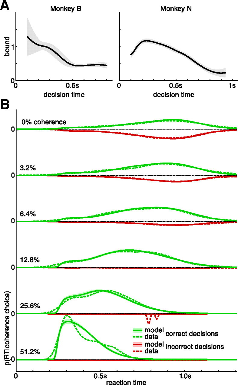
Fitted diffusion model bounds for both monkeys and reaction time distribution for monkey N. A, The plots show the mean bounds θ(t) [not the belief g_θ(t)], ±2 SDs indicated by the shaded area. The bounds for both monkeys have about the same magnitude, but the bound of monkey B is initially higher and collapses faster, while the bound of monkey N rises initially and gradually declines thereafter. This is reflected in the monkeys' reaction time distribution (Fig. 11), being peaked for monkey B and more spread out for monkey N. B, The reaction time distributions for monkey N are shown for correct and incorrect decisions (flipped along the abscissa) separately (smoothing and shaded areas as in Fig. 4). For higher coherences, the mass of the reaction time distribution for correct decisions increases, corresponding to a larger probability of correct choices (Fig. 4A). Also, they are skewed toward smaller reaction times, as reflected in the smaller mean reaction times (Fig. 4A). The distributions correspond to those predicted by a diffusion model with a boundary that varies as shown in A, under addition of a nondecision time.

The human data were fit using the same procedure, resulting in comparable fit quality for the reaction time distributions (Kolmogorov–Smirnov test; Table 1). For all subjects, the model explains >90% of the variance in the psychometric and chronometric curves (Table 1 for coefficients of determination).

Allowing the diffusion model bound to vary flexibly over time comes at the cost of introducing a large number of additional model parameters (12 for monkey fits; 11 for human fits) when compared with the commonly used DMs with constant bounds (3 model parameters) (Gold and Shadlen, 2002, 2007; Palmer et al., 2005). To evaluate whether this additional flexibility was justified, we used the AIC to compare our model to the simpler DM with constant bounds. The AIC compares the log likelihood of two models while penalizing for the number of parameters. Table 1 shows how the AIC of our model fit compares with that of a standard fit of a DM with constant boundaries. Based on this analysis, we conclude that the additional complexity of our model is justified.

The cost function

We now have all the quantities in place to infer the subjects' cost function, c(t), based on their fitted choice accuracies over time, using the decision-making model described above. For the monkeys, the use of a minimum reward time in the experimental setup makes the task a hybrid between a fixed-duration and a reaction time task, as no time is saved when making decisions before the minimum reward time has passed.

We first ensured that our method returns the correct cost function when known (Fig. 6) and then applied it to the monkeys' data, with the resulting cost functions shown in Figure 7. Several values of internal punishment are used, as those are not directly accessible from our data. The estimated cost functions are neither zero at all times nor take a single value that remains constant over time. Ignoring the initial uncertain transient, they are constant or only slightly increasing and start to ramp up significantly after ∼400 ms for monkey B and ∼650 ms for monkey N. The point in time at which the cost starts ramping up (Fig. 7) is close to the effective minimum reward times, that is, the points in time at which a correct decision will lead to immediate reward (effectively 651 ms for monkey B and 1084 ms for monkey N).

Figure 6.

Recovered cost function for simulated behavior. We ensured that our method returns the correct cost function by applying it to a set of simulated behaviors corresponding to known cost functions. Specifically, we generated choices and reaction times of 6000 trials using a diffusion model with time-varying boundaries, corresponding to the optimal behavior for a given cost function. The same procedure as for the analyzed datasets was used to estimate the cost function from this simulated data. The plots show both the true (dashed line) and the estimated cost function (solid lines, ±2 SDs) up to the 95% percentile of the reaction time distribution of the simulated data (mapped into decision time by removing the estimated nondecision time). The task was a reaction time task without minimum reward time, no penalty time, and an intertrial interval of t_i = 2s. The decision maker's nondecision time was simulated to be a constant t_nd = 2s. A reward of 1 was given for correct decisions, and no punishment occurred for incorrect decisions. The cost function was c(t) = −0.18 for the constant cost, c(t) = −0.2 + 0.15t for the linear cost, and c(t) = −0.2 + 0.2t² for the quadratic cost. The plots reveal an initial bias (<100 ms decision time) in the cost function estimate, which causes us to only report the cost function for the subjects after the first 100 ms.

One could hypothesize that the rising shape of the cost function is an artifact introduced by the minimum reward time. This hypothesis is not supported by the cost function for the human subjects (summary in Fig. 8; representative human subject in Fig. 7), which also rises even though the subjects' reaction time was not influenced by a minimum reward time. Similarly to monkey B, the estimated cost function for the human subjects dips briefly below zero for ∼150 ms, after which it rises continuously. Its rise is in the order of five times smaller than for monkey B and two times smaller than for monkey N within the same time span. This is reflected in the longer tails of the reaction time distributions for the human subjects when compared with the monkeys.

Figure 8.

Pooled cost function for human subjects. We estimate the cost function for each of the six human subjects separately and pool these estimates weighted according to their reliability. As for the monkeys (Fig. 7), we perform this procedure for various settings of the unknown internal reward. For either choice of this parameter, the cost estimate (shown with ±2 SDs) remains indistinguishable from constant until up to 200 ms, the dips slightly below zero for around 150 ms after which it rises almost linearly. This rise is significantly different from zero but much less pronounced than for the monkeys (Fig. 7; note the different scale).

Urgency signal independent of coherence

Our theory predicts that the decision termination rule is a function, g_θ(t), only of the decision maker's belief and time. Given knowledge of these two quantities, the termination rule should be the same on each trial, independent of its difficulty. This is surprising because the motion coherence is different on each trial, and one might expect that the termination rule would vary with difficulty, perhaps tipping the balance toward speed for easy conditions, toward accuracy on near threshold conditions, and maybe toward speed for conditions deemed similar to guessing. According to our theory, however, the termination rule is independent of motion coherence because the decision maker's belief about being correct is sufficient to estimate her expected reward, which is all that is required to decide on an appropriate course of action. Thus, even though the decision maker might infer the coherence on a trial-by-trial basis, this inference is not necessary for optimal decision making.

Importantly, the prediction of a termination rule that is independent of trial difficulty is consistent with the way this rule appears to be implemented at the neural level. The firing rate of neurons in the intraparietal cortex (LIP) seems to represent accumulation of evidence over time, as this rate, as a function of time, is consistent with a diffusion process with a deterministic drift (Shadlen and Newsome, 2001; Roitman and Shadlen, 2002; Churchland et al., 2011). This process of evidence accumulations terminates whenever the activity of one population (e.g., supporting H₁) reaches a threshold, which is independent of coherence and time. The fact that the threshold is independent of time would appear to contradict our prediction of collapsing bounds. However, LIP firing rates exhibit a time-dependent increase in firing rate that appears to affect all neurons, regardless of the choice they represent. This deterministic signal has been labeled an urgency signal (Churchland et al., 2008) because it is equivalent to our collapsing bounds. The symmetric collapsing bounds in the DM is approximated by the addition of a common urgency signal to competing accumulators. Instead of symmetric diffusion to an H₁ or H₂ bound, there are two (or more) diffusion processes that accumulate evidence bearing on these hypotheses (Gold and Shadlen, 2007). Unlike the value of the threshold, which is fixed over time, the urgency signal varies over time, thus implementing a time-varying collapse of the bound by bringing the firing rates of all neurons closer to a fixed threshold (Fig. 9A).

If our prediction is correct, the urgency signal should follow the same time course regardless of the value of coherence. This prediction is clearly supported by the data (Fig. 9B,C) (see Materials and Methods) (Churchland et al., 2008). The exact relationship between the urgency signal and the shape of the bound collapse in DMs depends on how the neural population activity encodes the accumulated evidence. As there are currently multiple proposed encoding schemes (Mazurek et al., 2003; Beck et al., 2008), we have not attempted to quantify this relationship.

It might seem that a decision rule that depends only on belief and time would predict that choice accuracy ought to be the same for all motion strengths given the same reaction time, but this is not the case. In fact, if we sort trials by evidence strength and then plot the choice accuracy over time for each of these evidence strengths separately, we find that the monkeys' choice accuracies differ between different evidence strengths (Fig. 10). It is critical to realize that, by sorting the trials by evidence strength, we effectively introduced additional information (the evidence strength) that is not available to the decision maker. In contrast, the decision maker has to establish her belief solely on the basis of the evidence received (δx_0…t in Eq. 27) and the prior over evidence strength alone. As we saw in Equation 27, this yields an expression for belief that depends on time but not on evidence strength. Nonetheless, we can use the additional information about evidence strength that was only available to the experimenters as a further test of our theory, which predicts quantitatively how choice accuracy changes over time per evidence strength (see Eq. 19). In particular, after an initial rise we expect this choice accuracy to decrease with time, in close agreement with the experimental data (Fig. 10). This is in stark contrast to a DM with a constant bound (that is, no urgency), which also predicts the choice accuracy to change with coherence, but remains constant over time for a given coherence (Eq. 19 with constant θ), contrary to what is evident in the data. Additionally, the good match between model and data also confirms that a single collapsing bound, independent of coherence, is sufficient to capture the observed data, as predicted by our theory.

Discussion

We have described how to find the optimal behavior in fixed-duration tasks, reaction time tasks, and a variant of the latter with a minimum reward time, based on knowledge of the internal reward contingencies and the temporal profile of the cost of accumulating evidence over time. Reversing this process and assuming optimal behavior allowed us to compute this cost for monkeys and humans performing a dynamic random-dot display reaction time task. The cost was found to be low initially but increased as time elapsed during a decision. All subjects assigned cost to the passage of time, and the cost per unit time was not constant. Put simply, during a decision, time costs more as time goes on.

To estimate the cost function from observed behavior, we assumed that the subjects act optimally to maximize their net reward rate, encompassing all expected costs and rewards. That is, the subjects need to (1) optimally accumulate evidence over time and (2) exploit a decision threshold that achieves reward-maximizing behavior. Requirement (1) means that subjects are able to consider all decision-relevant evidence presented to them to the best of their abilities (which might vary between subjects) without putting more weight on evidence provided early or late within a trial. Previous work has demonstrated this ability in the time frames present in our data (Kiani et al., 2008). For requirement (2), which is the acquisition of a reward-maximizing decision threshold, we can provide only indirect evidence. As shown in Figure 3, the optimal decision threshold for repeated trials, and tasks with varying difficulty, collapses over time. This pattern is also reflected in the subjects' fraction of correct choices, which also decreases as a function of time (Fig. 4B). In contrast, simpler strategies, such as the SPRT, predict the fraction of correct choices to remain constant over time. Thus, the subjects' behavior features the hallmarks of a reward-maximizing strategy, but a direct confirmation requires further work.

Our work complements many studies that use DMs to capture the speed/accuracy trade-off in perceptual decision making (Ratcliff and Smith, 2004; Palmer et al., 2005; Ditterich, 2006a,b; Gold and Shadlen, 2007). Importantly, we do not assume any particular model structure per se, but arrive at DMs with time-varying boundaries via considerations of optimal foraging. Thus, we do explain not only the observed behavior but also why it might be advantageous to behave as such.

Furthermore, we extend the SPRT of Wald and Wolfowitz and its extension to DMs. Wald and Wolfowitz showed that, for a constant cost function, accumulation of evidence to a stationary (i.e., flat) bound is the optimal policy for binary decisions—optimal in the sense of minimizing decision time, given a desired accuracy, on average. However, this property holds only when the reliability of the evidence is known such that evidence can be accumulated in units of a log-likelihood ratio until it reaches a desired level, or bound. Under this procedure, the passage of time does not affect the expected accuracy. Put another way, the time-dependent accuracy function is a constant because the bound represents a fixed level of belief.

In natural settings, however, the degree of reliability might vary across decisions, and we describe a rational approach to handle this variability. When the reliability of a source is not known in advance, having little evidence late within a trial implies a less reliable source. This in turn implies that the time-dependent accuracy is generally a decreasing function of time, because long trials tend to correspond to harder trials (Lai, 1988). Then, it becomes advantageous to stop accumulating more evidence to proceed to the next, potentially easier trial. In combination with an unknown degree of reliability, such rising cost increases the advantage of early stopping, resulting in a time-dependent accuracy that drops even faster as a function of time (Fig. 3D).

We addressed the optimal strategy for decision making with arbitrary costs of accumulating evidence when the degree of reliability is unknown. Frazier and Yu (2008) applied a similar dynamic programming technique to find optimal decision policies, but they assumed a constant cost function and a reliability of evidence known to the decision maker. They also considered a different trial structure in which correct decisions are only rewarded if subjects indicated their choice before a predetermined deadline. Rao (2010) applied reinforcement learning to learn optimal strategies for tasks similar to the ones we consider, but assumed a constant cost function and a long sequence of similar trials rather than using average-reward reinforcement learning. Our approach provides a normative framework that could, in principle, unite these approaches by the inclusion of stochastic deadlines, and by interpreting reinforcement learning as a stochastic approximation to our dynamic programming approach (Mahadevan, 1996).

Our theoretical framework allows us to estimate the cost of sampling and therefore argues in favor of the existence of such a cost but, independent of our model, the behavior of the monkeys also supports the existence of this cost. Assuming no such cost, there is no rational advantage in making decisions before the minimum reward time, as doing so will not reduce the waiting time until the next trial. At the same time, accumulating more evidence will always increase the choice accuracy and with it the expected reward. Despite this, both monkeys perform a large fraction of their decisions before the minimum reward time (>51% for monkey B, >92% for monkey N; Fig. 11). Moreover, in fixed-duration tasks, monkeys ignore information provided by the stimulus toward the end of long trials (Kiani et al., 2008). All of these behaviors would be rational if there exists a cost of accumulating evidence that, at some point within a trial, causes this cost to outweigh the expected increase in reward given more evidence.

Figure 11.

Full reaction time distribution of monkeys. The reaction time distributions are plotted using Gaussian kernel smoothing (width 20 ms). The arrows along the abscissa indicate the effective minimum reward time. For all decisions occurring before this time, administration of the reward is delayed until the minimum reward time has passed. Nonetheless, >51 and >92% of all decisions for monkey B and N, respectively, are made before the minimum reward time.

An important question is why the cost function takes the shape we observe here. One possible interpretation of the cost function is that, as discussed before, it corresponds to the effort of attending to the stimulus. Given its observed shape, this would imply that, initially, this effort is low but rises rapidly after a certain time. Interestingly, for the monkeys, the point at which the cost function rises seems to coincide with the minimum reward time, which differs for the two monkeys. Due to this dependence on task contingencies, the cost function cannot be fully explained by metabolic constraints. Rather, it might correspond to how the animal assigns its effort, or attention, to the task. Thus, the animal may distribute its resources such that the sampling cost is minimal within the minimum reward time and rises only thereafter.

As we discussed, the optimal decision-making framework predicts that the collapse of the bound on belief should only depend on time, and not on coherence. This prediction is supported by the finding that the urgency signal, which effectively implements a collapse of the decision bound, in LIP neurons is independent of the coherence. This point is especially important because many models of decision making assume evidence accumulation to a stationary bound (Link and Heath, 1975; Ratcliff and Smith, 2004; Gold and Shadlen, 2007), which is known to lead to too heavy tails of RT distributions and incorrect predictions for the RT on error trials (Laming, 1968). As we have shown, the normative solution—collapsing bounds or urgency signal in the neurophysiological realization—support slower mean RT on error trials and less skewed RT distributions, consistent with data.

Further tests of our theory will require experiments that aim at keeping the cost function constant while changing other task parameters that result in a predictable change in behavior. We believe it can be adapted to different task structures, such as asymmetric prior beliefs and payoff matrices, both of which modulate the optimal decision rule (Hanks et al., 2011). The ability to infer a time cost from behavior ought to allow future studies to separate the costs of evidence, time, and reward/penalty. It remains to be seen whether a coherent, normative framework can be implemented by neurons like the ones in LIP by simply incorporating a more elaborate cost-of-time signal in probabilistic neural models of decision making (Beck et al., 2008). It would also be interesting to explore extensions of this work to situations in which the strength of the evidence changes not only from trial to trial but also within a trial, and in which the variable of interest (direction of motion in our task) varies over time. Models using probabilistic population codes can perform optimal accumulation of evidence in this case (Ma et al., 2006; Beck et al., 2008, 2011), but how to set the bound to maximize reward rate in such models remains an open question.

References

- Akaike, 1974.Akaike H. A new look at the statistical model identification. IEEE Trans Automat Contr. 1974;19:716–723. [Google Scholar]
- Beck et al., 2008.Beck JM, Ma WJ, Kiani R, Hanks T, Churchland AK, Roitman J, Shadlen MN, Latham PE, Pouget A. Probabilistic population codes for Bayesian decision making. Neuron. 2008;60:1142–1152. doi: 10.1016/j.neuron.2008.09.021. [DOI] [PMC free article] [PubMed] [Google Scholar]
- Beck et al., 2011.Beck JM, Latham PE, Pouget A. Marginalization in neural circuits with divisive normalization. J Neurosci. 2011;31:15310–15319. doi: 10.1523/JNEUROSCI.1706-11.2011. [DOI] [PMC free article] [PubMed] [Google Scholar]
- Bellman, 1957.Bellman R. Dynamic programming. Princeton: Princeton UP; 1957. [Google Scholar]
- Bertsekas, 1995.Bertsekas DP. Dynamic programming and optimal control. Belmont, MA: Athena Scientific; 1995. [Google Scholar]
- Bogacz et al., 2006.Bogacz R, Brown E, Moehlis J, Holmes P, Cohen JD. The physics of optimal decision making: a formal analysis of models of performance in two-alternative forced-choice tasks. Psychol Rev. 2006;113:700–765. doi: 10.1037/0033-295X.113.4.700. [DOI] [PubMed] [Google Scholar]
- Britten et al., 1992.Britten KH, Shadlen MN, Newsome WT, Movshon JA. The analysis of visual motion: a comparison of neuronal and psychophysical performance. J Neurosci. 1992;12:4745–4765. doi: 10.1523/JNEUROSCI.12-12-04745.1992. [DOI] [PMC free article] [PubMed] [Google Scholar]
- Brockwell and Kadane, 2003.Brockwell AE, Kadane JB. A gridding method for Bayesian sequential decision problems. J Comput Graph Stat. 2003;12:566–584. [Google Scholar]
- Churchland et al., 2008.Churchland AK, Kiani R, Shadlen MN. Decision making with multiple alternatives. Nat Neurosci. 2008;11:693–702. doi: 10.1038/nn.2123. [DOI] [PMC free article] [PubMed] [Google Scholar]
- Churchland et al., 2011.Churchland AK, Kiani R, Chaudhuri R, Wang XJ, Pouget A, Shadlen MN. Variance as a signature of neural computations during decision making. Neuron. 2011;69:818–831. doi: 10.1016/j.neuron.2010.12.037. [DOI] [PMC free article] [PubMed] [Google Scholar]
- Cox and Miller, 1965.Cox DR, Miller HD. The theory of stochastic processes. New York: Wiley; 1965. [Google Scholar]
- Ditterich, 2006a.Ditterich J. Stochastic models of decisions about motion direction: behavior and physiology. Neural Netw. 2006a;19:981–1012. doi: 10.1016/j.neunet.2006.05.042. [DOI] [PubMed] [Google Scholar]
- Ditterich, 2006b.Ditterich J. Evidence for time-variant decision making. Eur J Neurosci. 2006b;24:3628–3641. doi: 10.1111/j.1460-9568.2006.05221.x. [DOI] [PubMed] [Google Scholar]
- Frazier and Yu, 2008.Frazier P, Yu A. Sequential hypothesis testing under stochastic deadlines. Advances in Neural Information Processing Systems 20. Paper presented at the Twenty-First Annual Conference on Neural Information Processing Systems; December; Vancouver, British Columbia, Canada. 2008. [Google Scholar]
- Gold and Shadlen, 2002.Gold JI, Shadlen MN. Banburismus and the brain: decoding the relationship between sensory stimuli, decisions, and reward. Neuron. 2002;36:299–308. doi: 10.1016/s0896-6273(02)00971-6. [DOI] [PubMed] [Google Scholar]
- Gold and Shadlen, 2007.Gold JI, Shadlen MN. The neural basis of decision making. Annu Rev Neurosci. 2007;30:535–574. doi: 10.1146/annurev.neuro.29.051605.113038. [DOI] [PubMed] [Google Scholar]
- Green and Swets, 1966.Green DM, Swets JA. Signal detection theory and psychophysics. New York: Wiley; 1966. [Google Scholar]
- Hanks et al., 2011.Hanks TD, Mazurek ME, Kiani R, Hopp E, Shadlen MN. Elapsed decision time affects the weighting of prior probability in a perceptual decision task. J Neurosci. 2011;31:6339–6352. doi: 10.1523/JNEUROSCI.5613-10.2011. [DOI] [PMC free article] [PubMed] [Google Scholar]
- Kiani and Shadlen, 2009.Kiani R, Shadlen MN. Representation of confidence associated with a decision by neurons in the parietal cortex. Science. 2009;324:759–764. doi: 10.1126/science.1169405. [DOI] [PMC free article] [PubMed] [Google Scholar]
- Kiani et al., 2008.Kiani R, Hanks TD, Shadlen MN. Bounded integration in parietal cortex underlies decisions even when viewing duration is dictated by the environment. J Neurosci. 2008;28:3017–3029. doi: 10.1523/JNEUROSCI.4761-07.2008. [DOI] [PMC free article] [PubMed] [Google Scholar]
- Lai, 1988.Lai TL. Nearly optimal sequential tests of composite hypotheses. Ann Statist. 1988;16:856–886. [Google Scholar]
- Laming, 1968.Laming DRJ. Information theory of choice-reaction times. London: Academic; 1968. [Google Scholar]
- Lee et al., 2007.Lee MD, Fuss IG, Navarro DJ. A Bayesian approach to diffusion models of decision-making and responsetime. In: Schölkopf B, Platt J, Hoffman T, editors. Advances in neural information processing systems. Vol 19. Cambridge, MA: MIT; 2007. pp. 809–816. [Google Scholar]
- Link and Heath, 1975.Link SW, Heath RA. Sequential theory of psychological discrimination. Psychometrika. 1975;40:77–105. [Google Scholar]
- Ma et al., 2006.Ma WJ, Beck JM, Latham PE, Pouget A. Bayesian inference with probabilistic population codes. Nat Neurosci. 2006;9:1432–1438. doi: 10.1038/nn1790. [DOI] [PubMed] [Google Scholar]
- Mahadevan, 1996.Mahadevan S. Average reward reinforcement learning: foundations, algorithms, and empirical results. Mach Learn. 1996;22:159–195. [Google Scholar]
- Mazurek et al., 2003.Mazurek ME, Roitman JD, Ditterich J, Shadlen MN. A role for neural integrators in perceptual decision making. Cereb Cortex. 2003;13:1257–1269. doi: 10.1093/cercor/bhg097. [DOI] [PubMed] [Google Scholar]
- Moreno-Bote, 2010.Moreno-Bote R. Decision confidence and uncertainty in diffusion models with partially correlated neuronal integrators. Neural Comput. 2010;22:1786–1811. doi: 10.1162/neco.2010.12-08-930. [DOI] [PubMed] [Google Scholar]
- Neal, 2003.Neal RM. Slice sampling. Ann Stat. 2003;31:705–767. [Google Scholar]
- Newsome et al., 1989.Newsome WT, Britten KH, Movshon JA. Neuronal correlates of a perceptual decision. Nature. 1989;341:52–54. doi: 10.1038/341052a0. [DOI] [PubMed] [Google Scholar]
- Palmer et al., 2005.Palmer J, Huk AC, Shadlen MN. The effect of stimulus strength on the speed and accuracy of a perceptual decision. J Vis. 2005;5:376–404. doi: 10.1167/5.5.1. [DOI] [PubMed] [Google Scholar]
- Rao, 2010.Rao RP. Decision making under uncertainty: a neural model based on partially observable markov decision processes. Front Comput Neurosci. 2010;4:146. doi: 10.3389/fncom.2010.00146. [DOI] [PMC free article] [PubMed] [Google Scholar]
- Ratcliff, 1978.Ratcliff R. Theory of memory retrieval. Psychol Rev. 1978;85:59–108. [Google Scholar]
- Ratcliff and Smith, 2004.Ratcliff R, Smith PL. A comparison of sequential sampling models for two-choice reaction time. Psychol Rev. 2004;111:333–367. doi: 10.1037/0033-295X.111.2.333. [DOI] [PMC free article] [PubMed] [Google Scholar]
- Risken, 1989.Risken H. The Fokker-Planck equation: methods of solution and applications. Ed 2. Berlin; New York: Springer; 1989. [Google Scholar]
- Roitman and Shadlen, 2002.Roitman JD, Shadlen MN. Response of neurons in the lateral intraparietal area during a combined visual discrimination reaction time task. J Neurosci. 2002;22:9475–9489. doi: 10.1523/JNEUROSCI.22-21-09475.2002. [DOI] [PMC free article] [PubMed] [Google Scholar]
- Rorie et al., 2010.Rorie AE, Gao J, McClelland JL, Newsome WT. Integration of sensory and reward information during perceptual decision-making in lateral intraparietal cortex (LIP) of the macaque monkey. PLoS One. 2010;5:e9308. doi: 10.1371/journal.pone.0009308. [DOI] [PMC free article] [PubMed] [Google Scholar]
- Shadlen and Newsome, 2001.Shadlen MN, Newsome WT. Neural basis of a perceptual decision in the parietal cortex (area LIP) of the rhesus monkey. J Neurophysiol. 2001;86:1916–1936. doi: 10.1152/jn.2001.86.4.1916. [DOI] [PubMed] [Google Scholar]
- Smith, 2000.Smith PL. Stochastic dynamic models of response time and accuracy: a foundational primer. J Math Psychol. 2000;44:408–463. doi: 10.1006/jmps.1999.1260. [DOI] [PubMed] [Google Scholar]
- Sutton and Barto, 1998.Sutton RS, Barto AG. Reinforcement learning: an introduction. Cambridge, MA: MIT; 1998. [Google Scholar]
- Vanderkerckhove et al., 2008.Vanderkerckhove J, Francis T, Lee M. A Bayesian approach to diffusion process models of decision making. In: Love B, McRae K, Sloutsky V, editors. Proceedings of the 30th Annual Conference of the Cognitive Science Society; Austin, TX: Cognitive Science Society; 2008. pp. 1429–1434. [Google Scholar]
- Vickers, 1979.Vickers D. Decision processes in visual perception. New York; London: Academic; 1979. [Google Scholar]
- Wald, 1947.Wald A. Sequential analysis. New York; London: John Wiley and Sons; Chapman and Hall; 1947. [Google Scholar]
- Wald and Wolfowitz, 1948.Wald A, Wolfowitz J. Optimum character of the sequential probability Ratio Test. Ann Math Stat. 1948;19:326–339. [Google Scholar]