Use of the gamma method for self-contained gene-set analysis of SNP data

Abstract

Gene-set analysis (GSA) evaluates the overall evidence of association between a phenotype and all genotyped single nucleotide polymorphisms (SNPs) in a set of genes, as opposed to testing for association between a phenotype and each SNP individually. We propose using the Gamma Method (GM) to combine gene-level P-values for assessing the significance of GS association. We performed simulations to compare the GM with several other self-contained GSA strategies, including both one-step and two-step GSA approaches, in a variety of scenarios. We denote a ‘one-step' GSA approach to be one in which all SNPs in a GS are used to derive a test of GS association without consideration of gene-level effects, and a ‘two-step' approach to be one in which all genotyped SNPs in a gene are first used to evaluate association of the phenotype with all measured variation in the gene and then the gene-level tests of association are aggregated to assess the GS association with the phenotype. The simulations suggest that, overall, two-step methods provide higher power than one-step approaches and that combining gene-level P-values using the GM with a soft truncation threshold between 0.05 and 0.20 is a powerful approach for conducting GSA, relative to the competing approaches assessed. We also applied all of the considered GSA methods to data from a pharmacogenomic study of cisplatin, and obtained evidence suggesting that the glutathione metabolism GS is associated with cisplatin drug response.

INTRODUCTION

Genetic association studies, in particular genome-wide association studies (GWAS) are a powerful approach in the search for common alleles with moderate effects on phenotypic traits. Over the last few years, GWAS have identified loci associated with numerous complex diseases.¹ However, the GWAS approach has limitations. Individual single nucleotide polymorphism (SNP) effects tend to be small and explain only a small proportion of the heritable variation in a phenotype,² making most SNP associations difficult to detect using the GWAS approach. To overcome these limitations of single SNP analysis, pathway or gene-set analysis (GSA) methods for SNP data evaluate the overall evidence of association of a phenotype with SNPs in all genes in a given molecular pathway or GS.^{3, 4} Such methods may enable the detection of subtle effects of multiple genes in the same pathway that may be missed by assessing each gene individually.

GSA methods were first introduced in the context of gene expression data analysis.^{5, 6, 7, 8, 9} Many of these methods were subsequently extended for the analysis of SNP data.^{10, 11, 12} Methods for GSA (for both expression and SNP studies) can be divided into two types: competitive and self-contained.⁶ Competitive or ‘enrichment' methods compare the results for genes within the GS with results for genes outside the GS (complement) to test the hypothesis that genes within the GS are associated with the phenotype more than genes outside the GS, whereas self-contained methods only consider results within a GS of interest to test the hypothesis that SNPs/genes in the GS are associated with the phenotype. For more details on competitive and self-contained GS methods, the reader is referred to Fridley and Biernacka³ and Wang et al.⁴ In this study, we have focused on only self-contained GSA methods to ensure fair comparison of methods testing the same null hypothesis.

In this manuscript we propose the use of the Gamma Method¹³ (GM) for GSA testing as part of either a one-step or two-step analysis strategy. We denote a ‘one-step' GSA approach to be one in which all SNPs in a GS are used to derive a test of GS association without consideration of gene-level effects; and a ‘two-step' approach to be one in which all genotyped SNPs in a gene are first used to evaluate association of the gene with the phenotype and then the gene-level associations are aggregated to test for association of the GS with the phenotype. A simulation study was completed to compare the use of the GM for GSA to several other self-contained GSA strategies, including both one-step and two-step GSA approaches, in a variety of scenarios. All of the methods considered are self-contained methods that can be utilized for binary, quantitative or time-to-event phenotypes. In addition to the simulation study, we performed GSA of data from a pharmacogenomic study of cisplatin drug response.

MATERIALS AND METHODS

The GM GSA approach

Self-contained GSA of SNP data can be performed using a ‘one-step' or a ‘two-step' approach. One-step analysis can be based on combining SNP-specific P-values to formulate a test of association of the GS with the phenotype, whereas a two-step analysis can be completed by performing gene-level tests of association and then combining the gene-level P-values to evaluate the association of the GS with the phenotype.

One of the most commonly used approaches for combining independent P-values is Fisher's method (FM).^{14, 15} Several extensions and modifications to FM have been proposed for summarizing results from genetic association studies.^{13, 16, 17, 18, 19} The FM can be shown to be a special case of the GM previously described by Zaykin et al.¹³ The GM is based on summing P-values transformed using an inverse Gamma(ω, 1) transformation. For a particular shape parameter ω, the test statistic is defined as where G⁻¹ is the inverse of a Gamma(ω, 1) cumulative distribution function.¹³ Application of different transformations to P-values before combining them into a test statistic varies the emphasis given to individual P-values, with more emphasis being given to P-values below a particular threshold. This threshold level, which has been referred to as the soft truncation threshold (STT), is controlled by the shape parameter ω.¹³ When ω is 1, the transformed P-values follow a χ²-distribution, and the GM becomes equivalent to FM with a STT value of 1/e. The shape parameter ω corresponding to a particular STT value can be calculated by solving 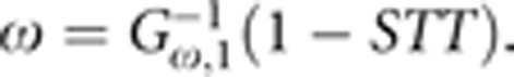By varying the shape parameter of the Gamma distribution, different transformations of P-values can be achieved, and thus the GM is a family of related methods with FM as a special case. Other P-value combination methods such as the truncated product method and rank truncated product method could also be considered for GSA. However, Zaykin et al¹³ found that the GM provided overall higher power in a simulation study. We therefore focus on the GM, including FM as a special case, for GSA as described below.

For application of the GM method to GSA, we investigated the use of the GM for combining SNP P-values for a one-step GSA or gene-level P-values for a two-step GSA. For the GM, we considered values of STT ranging from 0.01 to 1/e (ie, FM). For the two-step GSA, gene-level tests were performed using several different methods, before combining the gene-level P-values using the GM to evaluate association of the GS with the phenotype. Specifically, four commonly used methods for gene-level testing were assessed, including a global model with fixed effects (GMFEs), global model with random effects (GMRE),²⁰ principal components (PCs) analysis,²¹ and the minimum P-value (MinP) approach.

A limitation of the GMFE approach is that the model is only estimable when the number of predictor variables (eg, SNPs) is smaller than the number of subjects in the study (sample size). In contrast, the GMRE proposed for gene expression GSA by Goeman et al²⁰ is based on a random effects model that can accommodate a large number of SNPs. A continuous phenotype, Y, is modeled as Y∣X∼N(α1+Xβ,σ²l), where X represents a matrix containing the N SNP genotypes, coded in terms of the number of minor alleles, β represents a vector containing the effects of the N SNPs with each of the β_j's, j=1,…, N having a common distribution with mean 0 and variance τ². Under the null hypothesis of no association, the variance of the random effects is zero (τ²=0), which can be tested with a score test.²⁰ GMRE has been extensively utilized and shown to outperform other methods for GSA of mRNA expression data.²²

We also considered PC analysis for gene-level tests based on SNP data.²¹ In this approach, PCs are created using a linear combination of centered SNP genotypes (based on the number of minor alleles), with a subset of the PCs included as predictors in a regression model (eg, components that explain 80% of the variation). A gene-level test can then be based on a global test of association of the PCs with the phenotype.

Finally, the MinP, or maximum test statistic, over all SNPs in a gene is often used to represent the evidence of association with the gene in GS analyses.^{10, 11} This approach requires correctly accounting for gene size (number of SNPs) and LD between SNPs, as genes with more SNPs in lower LD are expected to have smaller MinP by chance, even in the absence of association between the genotypes and phenotypes.

In the second step of the two-step GSA methods, we combine the gene-level P-values using the GM with STT ranging from 0.01 to 1/e (ie, FM). All GS association P-values were determined empirically based on K permutations of the phenotype. This procedure leads to valid tests in the presence of differences in gene size and LD between SNPs or genes.

Other self-contained GSA approaches

All of the methods considered within the study are self-contained GSA approaches that can be applied to any type of phenotype (eg, binary case–control status, quantitative phenotype, time-to-event phenotype). Many of these methods were selected based on a prior study of GSA for mRNA expression data, which demonstrated that a GMRE, FM and PC approaches generally had the highest power among a number of self-contained GSA methods.²²

In addition to the one-step and two-step GM approaches described above, we also studied the performance of other one-step GSA methods. In particular, one-step GSA was also performed using PC analysis with components that explain 80% of the SNP variation and the GMRE method. For all one-step GSA methods, permutations were used to determine the empirical P-value for testing the association of the GS with the phenotype.

Case study: cisplatin pharmacogenomic analysis

The platinum agent cisplatin (CDDP) is a commonly used treatment for ovarian and lung cancer. To understand the pharmacogenomics of CDDP drug therapy and the role genetic variation has on the response to CDDP, the Coriell Human Variation Panel (HVP) lymphoblastoid cell lines (LCLs) from three racial groups were studied as described previously.^{23, 24} The quantitative drug response phenotype CDDP IC₅₀ (effective dose that kills 50% of the cells) was estimated using a four-parameter logistic model per cell line.²⁵

SNP genotyping was completed on the Illumina (San Diego, CA, USA) HumanHap 550K and HumanHap510S for the LCLs at the Genotyping Shared Resources at the Mayo Clinic in Rochester, MN, USA. In addition, publically available SNP data from the Affymetrix (Santa Clara, CA, USA) SNP Array 6.0 Chips were obtained for these cell lines. In total, before completing quality control, there were 1 698 648 unique SNPs on the three arrays, with 1328 SNPs mapping within 50 kb of the 27 genes in the glutathione metabolism pathway. After removing SNPs that failed quality control, 1272 SNPs in 27 genes remained for GSA of the glutathione metabolism pathway. Table 1 shows the number of SNPs in each of the 27 genes included in the analysis. Missing genotypes were imputed before analysis using the program fastPHASE.²⁶ The association of CDDP IC₅₀ and the glutathione metabolism pathway was assessed using the one-step or two-step GM approach with various STT values, along with the other self-contained GSA methods. The quantitative phenotype IC₅₀ and the genotype–phenotype association models were adjusted for gender, race, and five PCs within each race group to correct for possible population stratification effects. Empirical P-values were based on 1000 permutations.

Table 1. Single SNP and gene-level results for the CDDP pharmacogenomic study.

				Min. single SNP P-value		Gene-level association results
Chromosome	Gene	No. of SNPs in gene	No. of PCs	Observed	Permutation-corrected for multiple testing	GMRE	PCA	GMFEa
16	ABCC1	200	14	0.0099	0.543	0.184	0.504	1.000
10	ABCC2	44	4	0.0440	0.468	0.218	0.307	0.495
17	ABCC3	37	10	0.0889	0.904	0.902	0.817	0.371
13	ABCC4	526	34	0.0032	0.552	0.663	0.329	NA
6	GCLC	115	16	0.0228	0.782	0.780	0.513	9.75E-04
1	GCLM	25	3	0.0729	0.533	0.870	0.622	0.219
3	GPX1	2	1	0.9353	0.995	0.995	0.755	0.934
14	GPX2	4	2	0.0965	0.313	0.579	0.355	0.653
5	GPX3	61	7	0.0055	0.153	0.636	0.596	0.256
19	GPX4	7	2	0.3785	0.896	0.908	0.677	0.937
6	GPX5	16	3	0.0794	0.460	0.610	0.586	0.102
1	GPX7	21	4	0.1503	0.853	0.756	0.914	0.047
8	GSR	18	5	0.0147	0.171	0.330	0.173	0.218
20	GSS	13	3	0.0874	0.537	0.485	0.417	0.255
6	GSTA1	14	2	0.3756	0.848	0.757	0.977	0.361
6	GSTA3	40	4	0.0670	0.677	0.778	0.911	0.410
6	GSTA4	64	6	0.0461	0.652	0.312	0.392	0.021
1	GSTM1	5	3	0.0227	0.113	0.055	0.08	0.131
1	GSTM2	4	2	0.1858	0.554	0.411	0.354	0.452
1	GSTM3	11	2	0.0645	0.288	0.430	0.215	0.193
1	GSTM4	7	2	0.0779	0.310	0.161	0.248	0.046
1	GSTM5	7	2	0.0085	0.049	0.094	0.111	0.133
10	GSTO1	28	2	0.0506	0.304	0.134	0.07	0.143
10	GSTO2	27	3	0.0244	0.237	0.315	0.09	0.104
11	GSTP1	15	2	0.0015	0.008	0.008	0.001	0.011
22	GSTT2	2	2	0.5955	0.831	0.835	0.929	0.929
14	GSTZ1	16	3	0.0188	0.170	0.192	0.216	0.670

^aOnly computed for genes with P<N.

Simulation study for assessing GSA methods

Genotypes were simulated based on the observed SNP data in the glutathione metabolism pathway for the HVP LCLs from subjects of European descent. The 27 genes within the pathway were mapped to chromosomes, and haplotypes were phased using the program fastPHASE.²⁶ These haplotype frequencies were used to represent the underlying population. Three thousand haplotypes were simulated using the hapsim library in R (http://cran.r-project.org/web/packages/hapsim/index.html) based on these haplotype frequencies. Pairs of haplotypes were then assigned in a sequential manner to the 1500 individuals.

Case–control data sets with 500 cases and 500 controls were generated to evaluate GSA in the commonly used case–control study design. Using the simulated genotypic data for markers within the glutathione metabolism pathway, a binary phenotype (Z_i) for each subject i was generated conditional on their genotypic values from a Bernoulli distribution, Z_i∼Ber(p_i) with log(p_i/1−p_i)=X_i^Tβ. To generate data sets with 500 cases and 500 controls, the intercept in this model was selected such that the average probability of being a case was 0.50. From the cohort of 1500 subjects with a simulated binary phenotype (Z_i), 500 cases (Z_i=1) and 500 controls (Z_i=0) were randomly selected for analysis. The disease/phenotype models varied in the number and the size of the genetic effects, with odds ratios for individual SNP effects being 1.2 and 1.5 for small and moderate effects, respectively. All causal variants were observed in the data sets.

To assess the impact of the number of genes within a GS on the power and type I error rate, we also varied the size of the GS by removing 10 genes from the pathway for some simulations, so that the GS size was 17 or 27. LD between SNPs within the genes was also varied by tagging each gene at an r² of 0.60 or 0.90. The different simulation scenarios are listed in Table 2. Four ‘null' scenarios (all β_i=0) with no association of SNPs within the GS or pathway and 20 ‘non-null' scenarios (some β_i≠ 0) were simulated. In total, 1000 data sets were generated for each scenario, and all simulated data sets were analyzed with the GM one-step and two-step approaches, along with the other approaches. Individual SNP association P-values were based on the Armitage trend test. For GSA using the PC approach, the top k PCs needed to explain 80% of the variation in the SNP genotypes within each gene (for the two-step GSA), or GS (for the one-step GSA), were used as predictors of case–control status in the logistic regression model. The R library ‘globaltest' with the logistic model option was used to fit the GMRE (http://bioconductor.org/packages/2.6/bioc/html/globaltest.html). Empirical gene-set association P-values were based on 1000 permutations of the phenotype. Power and type I error rates were estimated based on a 0.05 significance level.

Table 2. Simulation scenarios.

		Number of SNPsa			Scenariob
Chromosome	Gene	r2=0.6	r2=0.9	All SNPs	1	2	3	4	5	In reduced gene set
16	ABCC1	43	83	200						Y
10	ABCC2	10	16	44						Y
17	ABCC3	21	28	37						Y
13	ABCC4	139	254	526						Y
6	GCLC	46	76	115	S	S	M	S	2 S	Y
1	GCLM	8	11	25						Y
3	GPX1	2	2	2	S					Y
14	GPX2	3	4	4						Y
5	GPX3	16	24	61						Y
19	GPX4	4	6	7	S	S	M		2 S	Y
6	GPX5	5	10	16						Y
1	GPX7	10	14	21						Y
8	GSR	7	10	18						Y
20	GSS	7	8	13						Y
6	GSTA1	1	3	14				S		Y
6	GSTA3	7	14	40				S		Y
6	GSTA4	16	25	64						Y
1	GSTM1	3	3	5						N
1	GSTM2	1	2	4						N
1	GSTM3	3	5	11						N
1	GSTM4	2	3	7						N
1	GSTM5	3	6	7	S					N
10	GSTO1	3	4	28						N
10	GSTO2	0	3	27						N
11	GSTP1	2	7	15						N
22	GSTT2	2	2	2						N
14	GSTZ1	5	8	16	S	S	M		2 S	N

^aThe number of SNPs per gene shows the total number of SNPs for each gene available in the original data, as well as the number of SNPs after tag SNP selection with an r² threshold of 0.6 or 0.9. Data sets analyzed in the simulations were those based on tag SNP selection with these two thresholds.

^bScenarios are described in terms of the number of small (S, odds ratio = 1.2) or medium (M, odds ratio = 1.5) SNP effects simulated in each gene:

Scenario 1: one small effect in each of five different genes (five causal SNPs).

Scenario 2: one small effect in each of one large gene and two small genes (three causal SNPs).

Scenario 3: one moderate effect in each of one large gene and two small genes (three causal SNPs).

Scenario 4: one small effect in each of three genes that are on the same chromosome (three causal SNPs).

Scenario 5: two small effects in each of three genes (six causal SNPs).

RESULTS

Simulation study

All methods had correct type I error rates (Supplementary Table 1). Summaries of the power for the various methods across different simulation scenarios are presented in Tables 3 and 4, and Figure 1. Supplementary Table 2 presents the entire set of results for all simulation scenarios. The distribution of power for each method over all investigated scenarios (disease association models 1–5 with different levels of LD and GS size) is summarized in Table 3, whereas the mean power of each method by scenario is shown in Table 4. The results show that, on average across the considered scenarios, the two-step approaches had higher power than the one-step approaches. The one-step FM (GM with STT=1/e), PC, and GMRE approaches had the lowest average power (mean power=0.57, 0.58 and 0.60, respectively). Their power was low compared with the two-step methods especially under scenarios with a smaller number of genes in the GS (ie, for the reduced GSs with 17 rather than 27 genes).

Table 3. Summary of power for PC-GM and other GSA methods.

Type of method	Method	Min.	First quartile	Median	Mean	Third quartile	Max.
Two-step	PC-GM
	STT=0.01	0.770	0.838	0.875	0.866	0.893	0.960
	STT=0.05	0.780	0.838	0.890	0.882	0.915	0.980
	STT=0.10	0.770	0.845	0.890	0.888	0.943	0.980
	STT=0.15	0.780	0.830	0.895	0.889	0.950	0.990
	STT=0.20	0.770	0.820	0.895	0.884	0.950	0.990
	STT=1/e	0.610	0.700	0.810	0.800	0.900	0.940
	GMRE-GM
	STT=0.01	0.720	0.770	0.880	0.850	0.933	0.960
	STT=0.05	0.730	0.798	0.895	0.873	0.943	0.980
	STT=0.10	0.760	0.800	0.890	0.879	0.953	0.980
	STT=0.15	0.740	0.798	0.880	0.878	0.963	0.980
	STT=0.20	0.690	0.785	0.900	0.863	0.953	0.970
	STT=1/e	0.540	0.630	0.780	0.770	0.910	0.960
	GMFE-GM
	STT=0.01	0.710	0.745	0.815	0.810	0.870	0.940
	STT=0.05	0.730	0.785	0.845	0.836	0.893	0.970
	STT=0.10	0.730	0.800	0.860	0.848	0.903	0.970
	STT=0.15	0.720	0.795	0.865	0.855	0.913	0.980
	STT=0.20	0.710	0.770	0.875	0.848	0.905	0.980
	STT=1/e	0.610	0.660	0.800	0.780	0.880	0.960
	MinP-GM
	STT=0.01	0.208	0.782	0.901	0.816	1.000	1.000
	STT=0.05	0.239	0.783	0.927	0.832	1.000	1.000
	STT=0.10	0.239	0.757	0.926	0.828	1.000	1.000
	STT=0.15	0.246	0.727	0.916	0.823	1.000	1.000
	STT=0.20	0.249	0.704	0.904	0.816	0.999	1.000
	STT=1/e	0.229	0.621	0.857	0.785	0.997	1.000
One-step	PC	0.100	0.290	0.500	0.580	0.970	1.000
	GMRE	0.070	0.290	0.620	0.600	0.990	1.000
	GM
	STT=0.01	0.187	0.782	0.908	0.810	1.000	1.000
	STT=0.05	0.137	0.712	0.902	0.786	1.000	1.000
	STT=0.10	0.122	0.587	0.862	0.742	1.000	1.000
	STT=0.15	0.107	0.492	0.812	0.706	0.999	1.000
	STT=0.20	0.097	0.419	0.752	0.674	0.998	1.000
	STT=1/e	0.082	0.251	0.529	0.569	0.949	0.987

Abbreviations: GM, Gamma Method; GMFE, global model with fixed effects; GMRE, global model with random effects; minP, minimum SNP P-value for gene.

For approaches that use the GM, the STT is listed after the name of the method.

For each GSA method, the distribution of power over all investigated scenarios (disease association models 1–5 with different levels of LD and gene set size) is summarized.

Table 4. Power for GSA methods under the five-disease-model scenarios of the simulation study, and P-values from application of the methods to the CDDP pharmacogenomic study.

		Power
Type of method	Method	Scenario 1	Scenario 2	Scenario 3	Scenario 4	Scenario 5	CDDP gene set P-value
Two-step	PC-GM
	STT=0.01	0.883	0.858	0.863	0.858	0.868	0.023
	STT=0.05	0.893	0.868	0.875	0.895	0.878	0.043
	STT=0.10	0.893	0.865	0.888	0.908	0.888	0.080
	STT=0.15	0.888	0.868	0.898	0.903	0.888	0.106
	STT=0.20	0.883	0.855	0.888	0.900	0.893	0.135
	STT=1/e	0.780	0.765	0.810	0.820	0.808	0.210
	GMRE-GM
	STT=0.01	0.858	0.855	0.835	0.853	0.848	0.176
	STT=0.05	0.870	0.880	0.858	0.880	0.875	0.223
	STT=0.10	0.883	0.885	0.860	0.878	0.890	0.279
	STT=0.15	0.878	0.880	0.860	0.880	0.890	0.310
	STT=0.20	0.848	0.855	0.848	0.870	0.893	0.322
	STT=1/e	0.755	0.763	0.763	0.765	0.785	0.358
	GMFE-GM
	STT=0.01	0.830	0.805	0.820	0.775	0.818	0.596
	STT=0.05	0.845	0.815	0.835	0.828	0.855	0.626
	STT=0.10	0.848	0.830	0.843	0.845	0.875	0.627
	STT=0.15	0.850	0.838	0.848	0.850	0.890	0.608
	STT=0.20	0.835	0.825	0.853	0.850	0.878	0.569
	STT=1/e	0.765	0.773	0.775	0.785	0.808	0.443
	MinP-GM
	STT=0.01	0.902	0.789	1.0	0.387	1.00	0.655
	STT=0.05	0.929	0.792	1.0	0.438	1.00	0.600
	STT=0.10	0.928	0.769	1.0	0.445	1.00	0.515
	STT=0.15	0.920	0.748	1.0	0.445	0.999	0.448
	STT=0.20	0.907	0.730	1.0	0.447	0.999	0.413
	STT=1/e	0.862	0.656	1.0	0.413	0.993	0.402
One-step	PC	0.497	0.307	0.995	0.141	0.949	0.294
	GMRE	0.622	0.300	0.997	0.114	0.980	0.230
	GM
	STT=0.01	0.908	0.789	1.000	0.352	1.000	1.000
	STT=0.05	0.901	0.728	1.000	0.299	1.000	1.000
	STT=0.10	0.860	0.606	1.000	0.246	1.000	1.000
	STT=0.15	0.811	0.506	1.000	0.215	0.998	1.000
	STT=0.20	0.756	0.428	1.000	0.192	0.993	0.991
	STT=1/e	0.535	0.254	0.986	0.143	0.925	0.432

For the simulation results, for each disease model (scenarios 1–5) power is averaged over the scenarios with different LD and gene set size.

Figure 1.

Comparison of power between the various two-step and one-step methods across all the simulation scenarios. All methods using the GM used the STT value of 0.15 (ω≈0.07654).

A comparison of a range of STT values for the GM for performing the second step of the two-step GSA (ie, summarization of the gene-level association P-values to a gene-set P-value) found that power was improved when a smaller STT was used, with STT between 0.05 and 0.20 providing the highest power for our simulation scenarios (Figure 2). On average, there was little difference in power between the four approaches (PC, GMRE, GMFE and MinP) for obtaining a gene-level P-value in step one of the two-step methods, with slightly higher mean power across scenarios for the PC approach over the fixed-effects (GMFE), random effects (GMRE) or MinP approaches. For the scenarios investigated, the level of LD used for SNP selection (and thus number of SNPs per gene) had little effect on the power of the GSA methods. In general, the various GSA methods were more powerful under scenarios with a smaller number of genes in the GS (ie, reduced GSs with 17 rather than 27 genes); however, this power increase was only observed for the two-step methods, and not when one-step analyses were performed.

Figure 2.

Plot of mean power (average across LD and gene-set size) by STT for the two-step GSA method PC-GM. Note that STT≈0.368 or 1/e corresponds to the commonly used FM for combining P-values.

Comparing the power across scenarios (Table 4), indicates that power of the one-step GSA methods and the MinP-GM two-step method was much more dependent on the true underlying disease model. In contrast, the other two-step approaches, such as the PC-GM approach, had consistently good power, relative to other approaches, for all scenarios assessed. Nevertheless, the one-step approaches performed very well for scenarios 3 and 5, with average power ranging from 0.986 to 1.0 and 0.925 to 1.0, respectively. These scenarios represent the case in which there are three moderate effects in three genes (one large and two smaller genes) (scenario 3) and the setting in which there are two small effects in each of three genes (scenario 5).

CDDP pharmacogenomic study

Results from the application of the one-step and two-step GM approaches as well as the other investigated GSA methods to the glutathione metabolism GS are presented in Table 4. The only method that produced a P-value less than 0.05 was the PC-GM approach with STT of 0.01 or 0.05 (PC.GM_0.01 P-value=0.023, PC.GM_0.05 P-value=0.043). This is consistent with the idea that the two-step GM method with small STT is generally more powerful than the other methods, as we had found in the simulation study. The one-step approaches resulted in the largest P-values, ranging from 0.23 to 1.0. In addition to the one-step approaches producing large GS P-values, the two-step approaches that used a full model with fixed effects to determine the gene-level P-values for association with IC₅₀ followed by the GM also produced large P-values for association of the glutathione metabolism GS with IC₅₀ (P-values ranging from 0.443 to 0.627).

Discussion and conclusions

In this manuscript we propose a novel GSA approach that uses the GM to combine gene-level P-values to determine the association of the GS with a phenotype. In our simulations the two-step GM approach, with either PC analysis or GMRE for determining gene-level P-values, followed by GM with a STT value between 0.05 and 0.20 for combining the gene-level P-values, had the best power across a range of disease models. The GM was previously proposed by Zaykin et al¹³ as a method for combining single SNP P-values in the context of genetic association studies. Here we extended this idea by considering the GM in combination with various gene-level tests of association, including fixed and random effects models and PC analysis, for a two-step GSA. We compared this approach with alternatives, including the GM applied to individual SNP P-values for a one-step GSA.

The presented simulation results showed that among the two-step GSA methods, the PC-GM, GMRE-GM and GMFE-GM preformed similarly, regardless of disease model (scenario); however, the performance of the MinP-GM approach depended greatly on the true underlying disease model (eg, high power when one moderate SNP effect within a gene and low power when small SNP effect within a gene). Under the scenarios considered in our simulation study, for the second step in the two-step GSA, combining gene-level P-values using the GM with STT values between 0.05 and 0.20 was more powerful than GM with STT=1/e (ie, FM). However, depending on the true underlying disease risk model, other STT values may lead to higher power. One option, therefore, is to consider a range of shape parameters for the Gamma transformation when combining P-values with the GM, selecting the minimum GSA P-value, and correcting for multiple testing. However, such an approach would introduce new challenges (eg, deciding on an appropriate correction for multiple testing) and may actually reduce power as a result of running more analyses requiring a correction for multiple testing.

The results of our simulation study also indicate that two-step methods are generally more powerful for detecting GS association as compared with one-step methods. For two of our simulated scenarios (scenarios 3 and 5), the one-step PC and one-step GMRE analyses were more powerful than the two-step analyses. In one of these scenarios there were three moderate effects in three genes, whereas in the other scenario, there were two small effects in each of three genes. For the remaining scenarios, the two-step GSA approaches were much more powerful than the one-step GSA approaches. Under the scenarios for which the one-step PC and GMRE methods were more powerful (scenarios 3 and 5), univariate analysis of individual SNPs with a Bonferroni correction for the number of SNPs in the GS has very high power to detect the SNP effects. Thus, the genetic effects in these two scenarios could have been detected by a typical GWAS single SNP analysis. In the remaining scenarios, where the two-step GSA approaches were much more powerful than the one step approaches, the analysis of individual SNPs had low power. These are scenarios for which analysis of each SNP individually may not have detected any significant association, but aggregation of the small effects via GSA may have identified significant GSs. These represent the situations that motivate GSA, and in these situations the two-step GSA was particularly advantageous.

GSA of data from the CDDP pharmacogenomic study using the two-step GM approach with gene-level P-values determined by PC analysis (PC-GM) suggested the glutathione metabolism GS is associated with the IC₅₀ phenotype (P<0.05). Although analysis of a single data set cannot be used to compare power of alternative approaches, the fact that these analyses provided stronger evidence for the association than did the other methods is consistent with the idea that the two-step GM approach, in particular the PC-GM method, is more powerful than other GSA approaches, as suggested by our simulation study.

In summary, GSA is a compelling approach for analysis of complex genetic data. On the basis of this study, we found that a two-step GM approach, with STT between 0.05 and 0.20, is a powerful approach for GSA, and in particular the PC-GM or GMRE-GM approaches. Once a GS is shown to be associated with a complex phenotype, further research is needed to assess the relationships between the SNPs and genes within the GS and the phenotype, and to reveal the biological pathways underpinning this relationship. GSA of existing GWAS data is expected to contribute to insights into the complex relationships between genomic variation and clinical phenotypes.

The authors declare no conflict of interest.

References

- Hindorff LA, Sethupathy P, Junkins HA, et al. Potential etiologic and functional implications of genome-wide association loci for human diseases and traits. Proc Natl Acad Sci USA. 2009;106:9362–9367. doi: 10.1073/pnas.0903103106. [DOI] [PMC free article] [PubMed] [Google Scholar]
- McCarroll SA, Kuruvilla FG, Korn JM, et al. Integrated detection and population-genetic analysis of SNPs and copy number variation. Nat Genet. 2008;40:1166–1174. doi: 10.1038/ng.238. [DOI] [PubMed] [Google Scholar]
- Fridley BL, Biernacka JM. Gene set analysis of SNP data: benefits, challenges, and future directions. Eur J Hum Genet. 2011;19:837–843. doi: 10.1038/ejhg.2011.57. [DOI] [PMC free article] [PubMed] [Google Scholar]
- Wang K, Li M, Hakonarson H. Analysing biological pathways in genome-wide association studies. Nat Rev. 2010;11:843–854. doi: 10.1038/nrg2884. [DOI] [PubMed] [Google Scholar]
- Subramanian A, Tamayo P, Mootha VK, et al. Gene set enrichment analysis: a knowledge-based approach for interpreting genome-wide expression profiles. Proc Natl Acad Sci USA. 2005;102:15545–15550. doi: 10.1073/pnas.0506580102. [DOI] [PMC free article] [PubMed] [Google Scholar]
- Goeman JJ, Buhlmann P. Analyzing gene expression data in terms of gene sets: methodological issues. Bioinformatics. 2007;23:980–987. doi: 10.1093/bioinformatics/btm051. [DOI] [PubMed] [Google Scholar]
- Efron B, Tibshirani R. On testing the significance of sets of genes. Ann Appl Stat. 2007;1:107. [Google Scholar]
- Dinu I, Potter JD, Mueller T, et al. Improving gene set analysis of microarray data by SAM-GS. BMC Bioinformatics. 2007;8:242. doi: 10.1186/1471-2105-8-242. [DOI] [PMC free article] [PubMed] [Google Scholar]
- Allison DB, Cui X, Page GP, Sabripour M. Microarray data analysis: from disarray to consolidation and consensus. Nat Rev. 2006;7:55–65. doi: 10.1038/nrg1749. [DOI] [PubMed] [Google Scholar]
- Holmans P, Green EK, Pahwa JS, et al. Gene ontology analysis of GWA study data sets provides insights into the biology of bipolar disorder. Am J Hum Genet. 2009;85:13–24. doi: 10.1016/j.ajhg.2009.05.011. [DOI] [PMC free article] [PubMed] [Google Scholar]
- Wang K, Li M, Bucan M. Pathway-based approaches for analysis of genomewide association studies. Am J Hum Genet. 2007;81:1278–1283. doi: 10.1086/522374. [DOI] [PMC free article] [PubMed] [Google Scholar]
- Chen LS, Hutter CM, Potter JD, et al. Insights into colon cancer etiology via a regularized approach to gene set analysis of GWAS data. Am J Hum Genet. 2010;86:860–871. doi: 10.1016/j.ajhg.2010.04.014. [DOI] [PMC free article] [PubMed] [Google Scholar]
- Zaykin DV, Zhivotovsky LA, Czika W, Shao S, Wolfinger RD. Combining P-values in large-scale genomics experiments. Pharm Stat. 2007;6:217–226. doi: 10.1002/pst.304. [DOI] [PMC free article] [PubMed] [Google Scholar]
- Fisher RA. Statistical Methods for Research Workers. London: Oliver and Boyd; 1932. [Google Scholar]
- Elston RC. On Fisher's method of combining P-values. Biomet J. 1991;33:339–345. [Google Scholar]
- Whitlock MC. Combining probability from independent tests: the weighted Z-method is superior to Fisher's approach. J Evol Biol. 2005;18:1368–1373. doi: 10.1111/j.1420-9101.2005.00917.x. [DOI] [PubMed] [Google Scholar]
- Zaykin DV, Zhivotovsky LA, Westfall PH, Weir BS. Truncated product method for combining P-values. Genet Epidemiol. 2002;22:170–185. doi: 10.1002/gepi.0042. [DOI] [PubMed] [Google Scholar]
- De la Cruz O, Wen X, Ke B, Song M, Nicolae DL. Gene, region and pathway level analyses in whole-genome studies. Genet Epidemiol. 2009;34:222–231. doi: 10.1002/gepi.20452. [DOI] [PMC free article] [PubMed] [Google Scholar]
- Yu K, Li Q, Bergen AW, et al. Pathway analysis by adaptive combination of P-values. Genet Epidemiol. 2009;33:700–709. doi: 10.1002/gepi.20422. [DOI] [PMC free article] [PubMed] [Google Scholar]
- Goeman JJ, van de Geer SA, de Kort F, van Houwelingen HC. A global test for groups of genes: testing association with a clinical outcome. Bioinformatics. 2004;20:93–99. doi: 10.1093/bioinformatics/btg382. [DOI] [PubMed] [Google Scholar]
- Gauderman WJ, Murcray C, Gilliland F, Conti DV. Testing association between disease and multiple SNPs in a candidate gene. Genet Epidemiol. 2007;31:383–395. doi: 10.1002/gepi.20219. [DOI] [PubMed] [Google Scholar]
- Fridley BL, Jenkins GD, Biernacka JM. Self-contained gene-set analysis of expression data: an evaluation of existing and novel methods. PLoS One. 2010;5:e12693. doi: 10.1371/journal.pone.0012693. [DOI] [PMC free article] [PubMed] [Google Scholar]
- Li L, Fridley BL, Kalari K, et al. Gemcitabine and arabinosylcytosin pharmacogenomics: genome-wide association and drug response biomarkers. PLoS One. 2009;4:e7765. doi: 10.1371/journal.pone.0007765. [DOI] [PMC free article] [PubMed] [Google Scholar]
- Niu N, Qin Y, Fridley BL, et al. Radiation pharmacogenomics: a genome-wide association approach to identify radiation response biomarkers using human lymphoblastoid cell lines. Genome research. 2010;20:1482–1492. doi: 10.1101/gr.107672.110. [DOI] [PMC free article] [PubMed] [Google Scholar]
- Gallant AR. Nonlinear Statistical Models. New York: Wiley; 1987. [Google Scholar]
- Scheet P, Stephens M. A fast and flexible statistical model for large-scale population genotype data: applications to inferring missing genotypes and haplotypic phase. Am J Hum Genet. 2006;78:629–644. doi: 10.1086/502802. [DOI] [PMC free article] [PubMed] [Google Scholar]
Associated Data
This section collects any data citations, data availability statements, or supplementary materials included in this article.