Recording from the same neurons chronically in motor cortex

Abstract

Two rhesus monkeys were implanted with silicon arrays of 96 microelectrodes. Neural activity was recorded periodically over a period of weeks to months. We have developed a method to determine whether single units in two separate recording sessions represent the same neuron. Pairwise cross-correlograms, the autocorrelogram, waveform shape, and mean firing rate were used together as identifying features of a neuron. When two units recorded on separate days were compared using these features, their similarity scores tended to be either high, indicating two recordings from the same neuron, or low, indicating different neurons. Although these metrics are individually weak, together they produce a strong classifier. Some neurons were recorded for >100 days. These monkeys performed a center-out reaching task, and we found that the firing properties of chronically recorded neurons were stable over time.

neurobiologists who do chronic extracellular recordings frequently observe similar activity recorded on the same electrode from day to day. Occasionally a single neuron will have some unusual characteristic, such as a distinctive waveform or some unusual and obvious firing property, that makes it clear that this same neuron is present in multiple sessions. The possibility that some neurons may be represented multiple times in a series of recording sessions creates a problem and an opportunity. Separately recorded neurons may not actually represent independent sources of data, so statistical tests that assume each unit is an independent sample may not be valid. However, if the same neuron could be identified as such across multiple sessions, it would be possible to combine data and thereby estimate the firing properties of that neuron with greater confidence. A sufficiently accurate metric of identity would allow all the recordings from a long series of sessions to be considered as a single population of neurons, with each identified unit contributing to the population for some portion of time.

A number of authors have attempted to identify the same neurons across recording sessions in a systematic way. The identification problem amounts to deciding, for each comparison between a sorted unit in one session and a sorted unit in another session, whether they represent the same neuron. Some authors have taken a qualitative approach, looking at waveform and sometimes interspike interval distribution information to identify examples with very stable characteristics (Chestek et al. 2007; Ganguly and Carmena 2009; Greenberg and Wilson 2004; Jackson and Fetz 2007; Schmidt et al. 1976; Williams et al. 1999). A few have developed classifiers that identify stable neurons systematically (Dickey et al. 2009; Tolias et al. 2007), but these methods are subject to severe tradeoffs between false negatives and false positives when the classifier is unreliable.

We have developed a new metric of unit identity using pairwise cross-correlograms between neurons in a simultaneously recorded population. It provides unit identification information comparable to that based on wave shape. Combining this metric with wave shape, autocorrelation shape, and mean firing rate, we are able to clearly identify whether two separately recorded units represent the same or different underlying neurons. We followed the identities of neurons across multiple sessions, in some cases for over 100 days.

The ability to track a large number of neurons across sessions allows us to address a fundamental question: how much do the tuning characteristics of neurons vary from day to day? There is a divergence of opinion in the literature as to whether the tuning characteristics of neurons are more or less fixed (Chestek et al. 2007; Ganguly and Carmena 2009; Greenberg and Wilson 2004) or whether they evolve continuously as part of a dynamic network that is only stable at the ensemble level (Carmena et al. 2005; Li et al. 2001; Rokni et al. 2007). We use our classifier to follow the same neurons over periods of weeks to months and find that the tuning of neurons to the direction of movement is stable over time.

MATERIALS AND METHODS

Chronic microelectrode implant.

Two male rhesus macaques were implanted with 96-channel microelectrode arrays (Blackrock Microsystems; Maynard et al. 1997). Monkey C was implanted in February of 2009 with a single array on the convexity of the motor cortex next to the central sulcus, with the lateral edge of the array ∼2 mm medial to the genu of the arcuate sulcus. The recordings reported here were done in March-April of 2010 and consist of six sessions recorded once a week on a day when the monkey did center-out movement tasks. Monkey F was implanted in April of 2009 with two arrays. One array was implanted in the same location as that of monkey C, targeting the primary motor cortex arm area. The other array was implanted further anterior and lateral, directly adjacent to the genu of the arcuate sulcus. This array was intended to target ventral premotor cortex. The recordings reported here were done in May 2009-March 2010. They consist of 40 sessions spread irregularly over that period. All animal procedures were approved by the institutional care and use committee of the University of Pittsburgh.

All activity was sorted offline using OfflineSorter (Plexon). OfflineSorter allows a variety of features to be used to sort; we used principal component distributions, peak/valley voltage, and voltage at specific time points. We used different features depending on the particular arrangement of waveforms on a given channel/day, and we only sorted units that were sufficiently distinct from noise and from each other. We identified 32–106 neurons per session from the combined activity of both arrays in monkey F and 14–22 neurons per session from the single array of monkey C.

Behavioral task.

Before implantation, each monkey was trained to do a center-out reaching task in a 3D virtual environment. They viewed a stereoscopic monitor (Dimension Technologies) that displayed a target sphere in its center and a cursor sphere that tracked the movement of an infrared marker (Northern Digital) taped to the back of the monkey's hand. To receive a water reward, the monkey had to complete a center-out movement. First, it had to move the cursor sphere to contact a central target for a required period randomly selected in each trial from 400–600 ms (monkey F) or 200–600 ms (monkey C). The target sphere would then be moved to a peripheral location selected randomly from a queue of 26 locations spread evenly in a sphere with radius 66 mm (monkey F) or 83 mm (monkey C). The monkey would then have to contact the peripheral target for 400–600 ms (monkey F) or 200–300 ms (monkey C). A failed trial resulted in the target being requeued. Monkey F also performed out-center trials, where the order of targets was reversed.

Tracking the same neurons.

An implementation of this algorithm has been posted to MATLAB Central as “Tracking neurons over multiple days”, identification no. 30113.

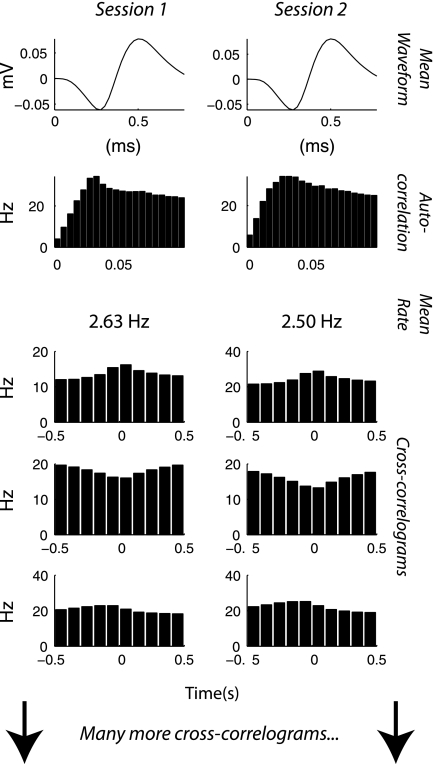
Let us consider the problem of determining whether a particular sorted unit in session 1 represents the same neuron as another sorted unit in session 2, one or more days later. In these data, we need only consider cases where the two units in question were recorded on the same electrode. This is because the interelectrode spacing on the Utah array is large (400 μm), so it is unlikely that one neuron will be recognized on two different channels. If the two units do represent the same neuron, there will be several indicators in the data that we can quantify. We expect that the mean waveform shape, the autocorrelation function, the mean firing rate, and the cross-correlograms with other neurons will be similar. An example of these parameters for the same neuron in two recording sessions is shown in Fig. 1. We quantify the similarity of the wave shape in the same manner as Jackson and Fetz (2007) as the peak value of the cross-correlogram between the average waveform shape in session 1 vs. session 2. This allows for changes in the overall size of the waveform and slight shifts in the time domain, which are common. The resulting coefficient is Fisher transformed (the arc tangent of the hypotenuse function) to make it more normally distributed.

Fig. 1.

The same neuron has been detected in 2 recording sessions 3 days apart. There are various indicators that this has happened. The cross-correlograms are between the target neuron and various other neurons that are present in both sessions. To line them up as we did above, we need to already know which neurons survived from session 1 to session 2. This problem is solved by an iterative procedure as described in Tracking the same neurons.

We estimate the autocorrelation function from 0 to 100 ms by binning at 5-ms resolution, exactly as is shown in Fig. 1. That gives us a 20-point vector for each session. To quantify the similarity of these vectors, we take the Pearson correlation coefficient between them. Again we Fisher transform to make the distribution more normal. The similarity of the mean firing rates is computed simply as the difference between the log of the mean rates. We take the log because mean firing rates follow an approximately log-normal distribution.

Because there are many neurons simultaneously recorded, there are many pairwise cross-correlograms. Those shown in Fig. 1 were chosen because they illustrate the strongest features for that neuron. The correlograms are computed for a range of ±0.5 s at 100-ms resolution. We found that this range captured the largest and most consistent features of the cross-correlograms, which tended to be positive and negative triangular bumps with lags near zero. The time-resolution represents a tradeoff between capturing finer features of the correlogram and computation time. These macroscopic features reflect common inputs rather than synaptic connections between neurons. To summarize all the cross-correlograms as a single metric, we first take Pearson correlations between presumed identical cross-correlograms in the same manner as we do for the autocorrelation functions. That means we are comparing one of the cross-correlograms on the left in Fig. 1 to the one immediately to its right, resulting in a single number for each pair. We Fisher transform those numbers and take the mean, resulting in a combined pairwise cross-correlogram similarity score.

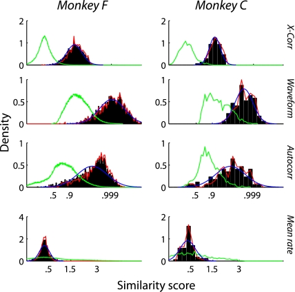
The distributions of each of the four scores are shown in Fig. 2. Because we have no data where we can be certain that two separate recordings represent the same neuron, we show the distribution for comparisons between recordings that are known to be different neurons (recordings from separate channels, green line). We also show several models of the same neuron distribution. The data points classified as same neuron are shown as a black histogram. The Gaussian computed by the expectation-maximization procedure (described below) is shown in blue and tends to match the black histograms, which is not surprising because they were classified as same neuron using that Gaussian as a model. We also show the synthetic data distribution in red, where we repeatedly classified the data using only three scores (detailed below) so that we could study the score we left out without invoking circular logic.

Fig. 2.

Distributions for each of the 4 types of similarity score for both monkeys. The y-axis of each plot is in units of probability density (the proportion of observations found in each bin, divided by the width of the bin). The x-axis indicates similarity score: correlation coefficient for X-corr, waveform, and autocorr; change in log mean rate for the bottom panel. The green line represents the distribution for comparisons between recordings from different channels, which are guaranteed to be different neurons. The black area represents similarity scores from the same channel on subsequent days that were classified by the algorithm as the same neuron. The red line represents the scores described in Synthetic data, where we ran the algorithm using only 3 of the scores so that we could validate the 4th score without creating circular logic. The blue line shows the Gaussian function representing the same-neuron distribution in the expectation-maximization procedure described in Tracking the same neurons.

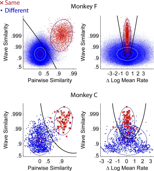
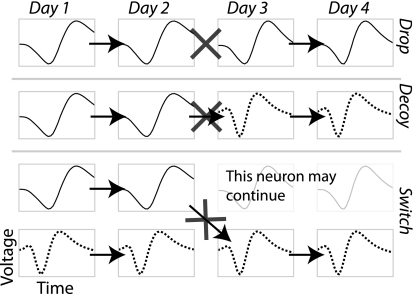
All four scores were combined with a quadratic classifier that computes an optimal decision boundary under the assumption that the underlying data can be modeled as a mixture of multivariate Gaussians. Ordinarily a training data set is used to fit these Gaussians. In our case, we have a great deal of known different-neuron data (comparisons across different channels, which cannot be the same neuron). However, we do not have any known same-neuron data. Therefore we used partially supervised expectation-maximization to fit a mixture of Gaussian models (Come et al. 2009; Lanquillon 2000). Our data set includes many points with known labels (cross-channel comparisons), whereas the remainder has mixed labels (within-channel, subsequent-day comparisons that might be the same neuron). Because the different-neuron data set is so large, it essentially dictates the shape of one of the Gaussians, and the other Gaussian converges very quickly onto a second cluster of points that lie away from the different-neuron distribution, putatively corresponding to the same-neuron comparisons. The location of the decision boundary and the contours of the two Gaussians are shown in Fig. 3, and the parameters of the Gaussians are summarized in Table 1. The decision boundary of the classifier is calibrated to produces a 5% error rate in the known different-neuron distribution. This may seem high but it is mitigated by the types of potential errors that occur in real recordings. Figure 4 illustrates the types of possible errors, which depend on how many neurons are present on a channel and how they emerge and disappear over time. Drop errors occur when the same neuron on two days is classified as two different neurons. Switch errors occur when the classifier switches the labels between two neurons, but at least one of them continues between days. This error happens rarely because the classifier will always label the session 2 neurons according to which session 1 neuron they fit best, so to produce a switch it essentially has to produce two errors simultaneously. When there are multiple surviving neurons, we consider all possible assignments of labels and choose the one that is most likely according to the Gaussian model of the similarity score. Decoy errors occur when one neuron disappears at the same time another appears, and they are classified as the same neuron. The 5% error rate that we use as a target applies only to instances where it is possible to make a decoy error, which are inherently unlikely.

Fig. 3.

Combining multiple similarity scores with a quadratic classifier. Each point represents a comparison between 2 units on 2 different days. We computed 4 similarity scores as described in Tracking the same neurons. These plots show projections of 2 scores at a time. Points are labeled according to whether they were classified as the same neuron. The same neuron/different neuron Gaussians estimated from the data are shown as contour plots. A 2-dimensional slice of the decision boundary that is used by the classifier is shown as a black line. The contours correspond to 25%, 50%, 75%, and 95% of the distribution. There are 6 unique combinations that could be shown; we chose the pairwise/wave scatterplot because they are the 2 most informative features, and we chose the mean rate/wave scatterplot because it illustrates the unique characteristics of the change-in-mean-rate feature.

Table 1.

Means and covariances of the Gaussian fits to the same-neuron and different-neuron distributions, shown as contour plots in Figure 3

	Monkey F					Monkey C
	Covariance Matrix				Mean	Covariance Matrix				Mean
	Same-neuron (red) cluster
Pairwise X-Corr	0.19	0.06	0.19	0.00	1.70	0.10	0.01	0.11	−0.02	1.61
Waveform		0.52	0.05	0.00	3.85		0.25	−0.03	−0.01	3.26
Autocorrelation			0.72	0.00	2.72			0.72	−0.02	2.56
Mean Rate				0.08	0.00				0.19	0.07
	Different-neuron (blue) cluster
Pairwise X-Corr	0.15	0.00	0.01	0.00	0.01	0.17	0.01	0.01	−0.01	0.03
Waveform		0.36	0.05	0.00	1.90		0.40	0.08	−0.04	1.78
Autocorrelation			0.67	0.00	1.06			0.32	−0.01	1.26
Mean Rate				2.74	0.02				1.57	0.08

Fig. 4.

Types of errors we can make while trying to label the same neurons over multiple sessions. Drop errors occur when the target neuron continues but the classifier fails to positively identify it across one of the gaps (indicated by the X). The original label is then a false negative until the target neuron actually disappears. Decoy errors occur when the target neuron disappears at the same time as a new neuron appears and the classifier mistakenly labels the new neuron as being the same as the old one. The label is then a false positive until the new neuron disappears. Switch errors occur when a distracter neuron is present simultaneously with the target and the classifier mistakenly switches the label to the distracter. Switch errors are the least likely because they essentially require the classifier to simultaneously make a drop and a decoy error.

When we use cross-correlograms to assess the identity of many neurons across two sessions, changes in labeling across days need to be considered. For instance, two neurons sorted on channel 1 might be labeled “unit 1a” and “unit 1b.” On the next day, their labels may be exchanged by the investigator doing spike sorting, or unit 1a may have disappeared and unit 1b is now labeled 1a. If we then wish to assess whether some other unit, for example unit 2a, is the same in session 1 and session 2, there is a problem with the cross-correlogram similarity metric. The cross-correlogram between unit 2a and unit 1a in session 1 will be different than in session 2, even if unit 2a is actually still the same neuron. We solved this problem with an iterative procedure, making an initial assumption that, wherever the unit labels are the same between session 1 and session 2, they represent the same neuron. We then used our four-score classifier to identify which units putatively corresponded to the same neurons from session to session. This set of identities was then used to relabel all the units, and classification was performed again, under the assumption that the number of labeling errors will be reduced with each iteration. If this assumption is correct, the labeling will tend to converge, which it does after a few iterations. We found that >99% of the unknown identities did not change after the first iteration.

The classification procedure we have described so far determines whether each recorded unit in session 1 represents the same neuron as a unit in session 2. We tracked the same neurons across many sessions by repeatedly applying this classifier to adjacent pairs of recordings. When following neurons across many sessions, it is theoretically possible that better choices could be made by considering the entire data set at once and employing a graph-cut algorithm. We chose not to pursue this approach because the “soft” assignment (probability same/probability different) of the Gaussian model was so bimodally distributed that almost any decision procedure would produce the same answers. There is a related concern that some neurons may be recorded for a few sessions and then become undetectable for some period of time, only to return later. Such a neuron would be given two labels, one for each period it was continuously recorded. We chose not to attempt to correct such situations because the most important metric of similarity (cross-correlations) works best when there are many identical neurons present in both sessions, which we can use to construct comparable cross-correlograms (Fig. 1). Also, attempting to link such segments dramatically increases the potential for errors because a long series of recordings will contain many segments of recording that could be linked together erroneously.

Synthetic data.

Because we could not test our algorithm with data where the identity of neurons across days is known, we constructed a synthetic data set by using the actual data to capture the variability in these metrics across separate recording sessions. There are four similarity scores: pairwise cross-correlation, wave shape, autocorrelation similarity, and mean firing rate. We computed a synthetic true-positive data set for one score at a time by ignoring that score and using only the other three to classify the entire data set. The points classified as same-neuron can then be used as a synthetic same-neuron distribution for the score we left out. To avoid introducing a lot of errors, we defined a conservative three-score boundary that would drop 25% of the points classified as positives by the full four-score classifier. To understand how this works, let us consider a simplified example where we only have the two scores shown in Fig. 3, top left. We are going to use just the pairwise similarity (x-axis) to classify a set of points as positive. That means we will draw a vertical line and classify everything to the right of it as positive. We can then use these points as a true-positive data set for the wave similarity score.

By using this technique four times, we create four different pools of synthetic true-positive scores. We then recombine a random value from each pool to create artificial data points. With these synthetic true-positive points and the known-negative distribution (neurons on separate channels), we have a complete data set where the ground truth is known. This technique for creating synthetic data creates a specific kind of bias attributable to the fact that there is some correlation between the different scores, as can be seen in the slight tilt of the red cloud in Fig. 3. When we use three scores to generate a known same-neuron distribution for the fourth, we throw away 25% of the positive category that were worst with respect to the three scores. Even though we did not consider the fourth score in deciding what to throw away, because of the presence of correlation, we end up with a slightly nonrepresentative set of points with respect to the fourth score. On average, this technique biases the distribution of fourth metric 0.1 standard deviation upward.

Long-term accuracy.

To extrapolate the various error rates to performance in a long series of recordings, we need to know how many neurons disappear from our electrodes each day, how likely we are to record n neurons on the same channel, and how often the decoy error scenario occurs (Fig. 4). These parameters were estimated using the labels produced by the full four-score classifier. Using the results in this way creates a bias with respect to decoy errors; if the classifier frequently makes an error when presented with a decoy neuron, then we will tend to underestimate how often decoy scenarios actually occur because each of these errors will result in one less decoy reported in the data. We set the decision boundary of the classifier to target a 5% decoy error rate, as described in Tracking the same neurons. Therefore, we assume that decoy scenarios actually occur 5% more often than they appear in the data. We modeled the turnover rate (the proportion of the population replaced daily) as an exponential decay that became smaller as a neuron was recorded for a longer duration, which corresponded to tendency in the data for a core group of stable neurons to persist from day to day, coexisting with another group of more marginal neurons that turned over frequently. The estimates for monkeys F and C are turnover rate (for the average gap between sessions), 15%/35%; additional neurons per channel, 0.4/0.4; and percent of neurons ending in a decoy-prone situation, 11%/10%. We used these parameters along with the drop, decoy, and switch rates from synthetic data to extrapolate the performance of the classifier over time. In results we use the terms “false negative” and “false positive” in the context of long-term data, defining the false positive rate as the proportion of labels that exist at a given time that are on the wrong neuron. The false-negative rate was defined as the number of labels no longer in existence even though their target neuron still is, divided by the number of labels currently in existence.

Preferred directions.

We estimated the preferred direction of each neuron on each day it was recorded by fitting a linear model: λ = β₀ + β_xx + β_yy + β_zz, where λ is the firing rate of the cell, x, y, and z are the target direction, and the β terms are the parameters of the model. The preferred direction (PD) of the cell is the vector <β_x, β_y, β_z>. We generated a measurement error distribution for this cell by bootstrap resampling the residuals of the fit on a per-trial basis. This method will incorporate the variability in firing rates that is caused by variability in kinematics. In this model, nonlinearity in the tuning function is considered part of the noise term, so the model will tend to slightly overestimate the amount of measurement error. We will need this measurement error cloud when we make two observations of the PD of the same neuron so that we can associate a level of uncertainty with our estimate of the angle between observations. Because these PDs are three-dimensional, the effect of measurement error is somewhat complicated. If two PDs are 90° apart, the measurement error is as likely to make the angle smaller as bigger. If they are more than 90° apart, measurement error will tend to bring the observations closer together. We solve this problem by calculating a “pure measurement error” distribution for each comparison, rotating the measurement error cloud of PD 2 so that its mean matches the mean of the PD 1 cloud and taking repeated samples from each distribution to compute the angle between them. In results, we will test two null hypotheses about the evolution of PDs over time: that they are unchanging, or that they change in a random walk. To test the no-change hypothesis, for each case where a neuron was observed twice, we computed a quantile for the observed change in PD, indicating where it lies in the appropriate measurement error distribution. If the true PD is unchanging, these quantiles should be uniformly distributed. To test the random-walk hypothesis, we assumed that the real change in PD could be modeled as a step each day in a random direction with a Gaussian-distributed step size. The step size was estimated using comparisons between adjacent sessions (only available in monkey F), taking into consideration the fact that observed PD change equals real change plus measurement error. We then generated a random-walk distribution numerically and added the appropriate measurement error distribution to it. Again, we compared the observed change in PD to the numerically generated distribution and computed a quantile. The uniformity of these quantiles was assessed with a K-S test.

RESULTS

Classification accuracy.

Figure 2 shows the separation of each individual score into a high-similarity and low-similarity group. Of particular note is the red line, representing the synthetic data distribution. We generated this distribution for each score using only the other three scores. It is therefore our most valid estimate of the true shape of the same-neuron distribution for each score. The accuracy of our algorithm is assessed in several ways, each of which is subject to different kinds of bias. The simplest approach is to generate a data set where the ground truth is known by splitting each recording session in half and comparing the two halves as though they were separate sessions. This results in a high-similarity cluster from comparisons between the same neuron in the first and second half of the data and a low-similarity cluster from comparisons between different neurons. Compared with multi-day data, the high-similarity cluster is likely to be more tightly distributed and further from the low-similarity cluster because the similarity metrics we are using are likely to change less between the first and second half of a single session than across the interval between sessions. For this data set we changed the initial conditions of the iterative identification procedure by randomizing the unit labels so that the classifier was not initialized with the correct answer. Testing our classification algorithm using split session data gave zero errors in monkey C and a 0.005% overall error rate in monkey F.

Without knowing the ground truth, there are some ways to estimate the error rates in the real data. 1) Estimate the decoy error rate using comparisons across separate electrodes, which can't be the same neuron. 2) Estimate the drop rate by modeling the data as a mixture of Gaussians. 3) Estimate the drop rate with synthetic data.

We use method 1 to set the classification boundary with a target decoy error rate of 5%. Where we set the classification boundary amounts to a tradeoff between drop errors and switch or decoy errors. A 5% target for the decoy rate heavily favors the drop rate, which ends up <1%. The decoy error rate in a real data set will be the product of 5% and the rate at which the decoy error scenario occurs (see Fig. 4), which is rare.

For method 2, we used the Gaussian models shown in Fig. 3. For every same-channel comparison classified as a negative, we estimated the probability that it was actually an unusually inconsistent single neuron using the density of the same-neuron and different-neuron Gaussians. By taking the mean of these probabilities we estimated the overall drop rate (Table 2).

Table 2.

Drop rate table

	Monkey F					Monkey C
	Pair	Wave	Auto	Rate	Not	Pair	Wave	Auto	Rate	Not
	Gaussian Model
Pairwise X-Corr	0.04	0.01	0.04	0.02	0.12	<0.01	<0.01	0.02	<0.01	0.16
Waveform		0.22	0.13	0.16	0.02		0.31	0.13	0.24	<0.01
Autocorrelation			0.40	0.37	<0.01			0.35	0.35	<0.01
Mean Rate				0.59	<0.01				0.53	<0.01
All	<0.01					<0.01
	Synthetic Data
Pairwise X-Corr	0.01	<0.01	0.01	<0.01	0.02	<0.01	<0.01	<0.01	0.01	0.08
Waveform		0.09	0.03	0.04	0.00		0.23	0.07	0.15	<0.01
Autocorrelation			0.23	0.20	<0.01			0.31	0.31	<0.01
Mean Rate				0.68	<0.01				0.73	<0.01
All	<0.01					<0.01

Each entry indicates the drop rate for a quadratic classifier based on 1 or more scores. We assessed drop rate by modeling the data as a mixture of Gaussians (method 2 in the text) or using synthetic data (method 3 in the text). Performance is shown for each metric of identity, each combination of 2, and for the full classifier based on all 4 combined. Single-metric performance is on the diagonal. 2-Metric performance is indicated by the combination of row and column labels. The “Not” column indicates the performance of a classifier with the 3 scores other than the row label. The decoy rate was always 5% (method 1 in the text) due to the way we set the classification boundary.

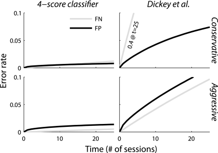
For method 3, we constructed a synthetic data set as described in materials and methods, applied our classifier, and calculated the drop rate (Table 2). The accuracy results are broadly similar to method 2. Pairwise cross-correlograms are the most important metric, followed by waveform, autocorrelation, then mean rate. We then extrapolated the synthetic data error rates to generate the long-term false-negative and false-positive scores shown in Fig. 5 (see Long-term accuracy). For comparison, we implemented a similar algorithm that uses the same wave shape score as ours and a similar autocorrelation score (Dickey et al. 2009). The long-term false-positive rate of the Dickey et al. algorithm was different than they reported because of differences in the way we tested the classifiers. Dickey et al. (2009) assessed long-term false positives by constructing a synthetic data set where each day a neuron from a different channel was used. To get a false positive after n days, the classifier would need to make n errors in a row. We assessed long-term error rates by estimating the various error rates for single comparisons (Table 2), then estimating how often various error scenarios would occur (Fig. 4). Using this approach, we find error rates tend to increase over longer periods of recording. Figure 5 shows performance for both a conservative threshold, which minimizes false positives, and an aggressive threshold, which minimizes false negatives. The aggressive threshold is similar to the one used in Dickey et al. (2009), targeting a ∼25% false-positive rate. The conservative threshold targets 5%. We used the conservative threshold for all classification in the remainder of this paper.

Fig. 5.

Long-term accuracy in a synthetic data set for our method and a similar method with 2 classifiers (Dickey et al. 2009). Here we define accuracy in terms of whether after x days a label is still correct. False negatives (FN) are cases where the label is gone but the target neuron is still around. False positives (FP) are cases where the label is on the wrong neuron, whether or not the original target is still present. In the top row, the classification boundary was set conservatively, targeting a 5% decoy rate. In the bottom row, the classification boundary was set aggressively as described in Dickey et al. (2009). The figures on the right have a significantly higher false-positive rate because they experience a nonnegligible number of switch errors, which accumulate rapidly. False-positive errors tend to be more damaging in studies that examine the properties of neurons over time, but a high false-negative rate will be inefficient because many neurons will not be tracked as long as they could be.

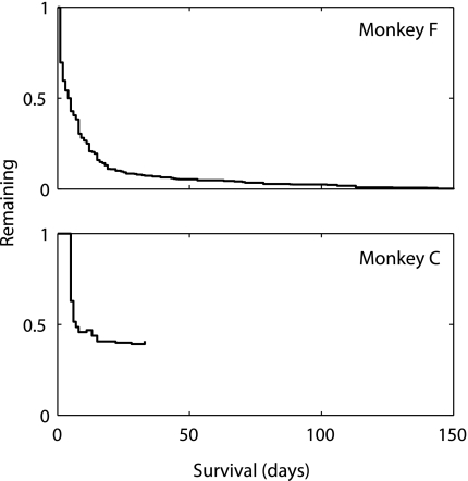
Our classification algorithm identified 760 unique neurons in monkey F and 35 in monkey C. The lengths of observation for these neurons are shown in Fig. 6. Most neurons were recorded for less than 30 days, but some in monkey F were recorded for over 100.

Fig. 6.

Observation lengths for recorded neurons. X-axis indicates recording duration for a single neuron. Y-axis indicates the number of neurons that were recorded that long, divided by the number of neurons that could have been recorded that long. We identified 760 unique neurons in monkey F out of 2892 sorted units recorded over 40 sessions. We identified 35 unique neurons in monkey C out of 104 sorted units recorded over 6 sessions. Monkey C had a smaller but more stable population.

Tuning parameters.

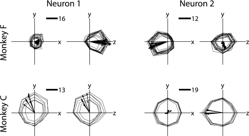
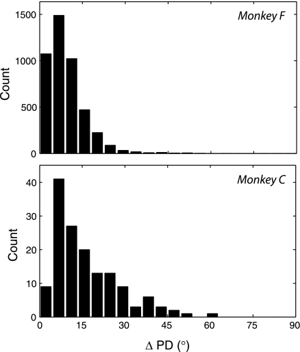
With the same neurons identified over a long-term data set, we can evaluate the stability of the directional tuning of these cells over time. Examples of tuning profiles for neurons that were tracked for a particularly long time are shown in Fig. 7. These examples show low variability in their tuning function between sessions. For each day that each neuron was recorded, we fitted a cosine tuning model describing a linear relationship between the direction of movement and the firing rate of one cell (see Preferred directions). Figure 8 shows histograms for the PD variability between two or more sessions, for all recorded cells. It was necessary to exclude units with weak or inconsistent modulation because changes in their PDs reflect more measurement error than real change. We assessed measurement error by bootstrapping the residuals of the cosine tuning fit (see Preferred directions) and excluded all comparisons where the uncertainty in our estimate of PD change was greater than 10°. This excluded 49% of the population in monkey F and 17% of the population in monkey C. The excluded set is based on the measurement error, not change in PD, so we are not limiting the potential for real variation in the PD across sessions; a neuron with a strong preferred direction in one session could have an equally strong but altered preferred direction in the next session.

Fig. 7.

Directional tuning profile across multiple sessions, 2 neurons from each monkey. The mean firing rate for each target is displayed in the direction of that target. There are 26 targets in 3D space; here we see x–y and z–y slices. Firing rate profiles from each single neuron are rendered simultaneously for all sessions where that cell was recorded. Arrows indicate preferred directions (PDs) from model fit. Scale bars indicate number of spikes per reach. The neurons shown are the first 2 neurons from each monkey that were recorded for at least 14 days with a mean preferred direction measurement error of <5°. Low measurement error does not necessarily limit the amount of variation in PD across sessions.

Fig. 8.

Observed differences in PD of single neurons across sessions. PD is the vector indicating the target that would theoretically elicit the maximal firing rate from the neuron according to a cosine-tuning model fitted from the data. X-axis indicates the absolute difference in PD. Y-axis indicates histogram bin counts. The histogram includes the angle between every possible pair of 2 observations of the PD of the same neuron. Comparisons are only included where the uncertainty in our estimate is <10° according to the bootstrap distributions described in Preferred directions. This does not constrain the potential variation in PD across sessions. Note that, in 3 dimensions, 2 PD vectors chosen at random are much more likely to have an angle difference of around 90° than around 0°.

Figure 8 shows that PD variability is low, generally < 30°. In assessing these changes in PD, we consider three hypotheses: 1) The PD is static, and all variation is due to measurement error. 2) The PD experiences slight real variation, which accumulates over time to create a random walk. 3) The PD experiences slight real variation, which accumulates, but it is tethered to an underlying intrinsic value that does not change.

Hypothesis 1: the PD is static.

If the true change in PD is always zero, then the observed changes should follow the distribution of measurement error that we computed by bootstrapping the residuals of the cosine tuning fit. We can compare each observed change in PD to the measurement error distribution described in materials and methods and compute a quantile. If the observed changes were due only to measurement error, these quantiles would be uniformly distributed. Using a K-S test, we rejected this hypothesis (P < .01).

Hypotheses 2: the PD experiences real variation that accumulates over time.

We extrapolated a series of distributions of PD changes from the 1-day changes by assuming that PD change represented a random walk plus measurement error, as described in materials and methods. This distribution was tested against the data with a K-S test in the same way we assessed hypothesis 1, and again it is a bad fit (P < .01). This rejects hypothesis 2.

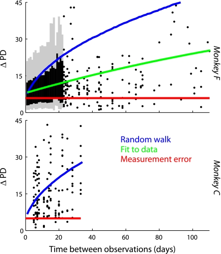
Figure 9 shows a scatterplot of the relationship between observation interval and PD difference. The expected-value lines associated with hypotheses 1 and 2 are shown and are above the mean of the data, visually confirming the results of the K-S test. This leaves us to conclude that, although there is real variation in PDs, they are tethered to underlying intrinsic PDs.

Fig. 9.

The relationship between observation interval (x- axis) and difference in PD (y-axis). This is the same data as Fig. 8, scattered out over time. Each point indicates that 2 observations were made of the PD of the same neuron x days apart, and the angle between the 2 observations was y degrees. For monkey F, we summarized dense regions of the scatter plot with a gray line indicating 95% of distribution and a black line indicating 66%. Red line shows the expected average difference in PD if all change is caused by measurement error. Blue line indicates a hypothetical trend assuming that the changes in PD accumulate over time (see Preferred directions for details). Green line shows a simple nonlinear function fit to the data, y = b₁ − b₂·exp(b₃·x). Although there is a limited amount of accumulation, it is significantly below the distribution associated with the blue line, indicating that there is an intrinsic unchanging preferred direction for each cell.

DISCUSSION

This report takes a series of extracellularly recorded populations and attempts to identify in every case whether an earlier session/later session pair represents the same neuron. Most past work on this topic has attempted to identify a minority of stable cells that can be reliably tracked, leaving the rest of the population in the category of “uncertain”. The four features we used are individually weak classifiers, but, because they represent independent sources of information, they can be combined into a strong classifier. For example, mean firing rates can indicate that two units are definitely not the same neuron, but they can never give high confidence that they are the same. The mean firing rate of a single neuron tends to be consistent from day to day, but the expected difference in mean rate between two different neurons is also zero (Fig. 3). Thus, if two units on two days have a very different mean rate, then they are almost certainly different neurons; but, if they have a similar mean rate, we cannot be certain that they are the same neuron. By itself, mean firing rate would be an inaccurate way to identify neurons, but when combined with other metrics it contributes useful information. With four different metrics of similarity, we can produce a very strong classifier that can follow neuron identity throughout entire population, not just the largest units with the most consistent characteristics.

Estimating identity for the entire data set not only allows us to take full advantage of the data we have collected, but also it will allow us to treat the entire chronic series as a single data set for the purpose of network analysis. The analysis of multi-observation data, where different subsets of a network are observed in overlapping intervals of time, has been a topic of growing interest (Lambiotte et al. 2009; Mucha et al. 2010). When using this algorithm in the context of network analysis, it is important to keep in mind that units that possess no functional connectivity may be less trackable because of the lack of features in their cross-correlograms. Setting aside these future directions, the most obvious immediate application of a unit identification algorithm is to determine whether the firing properties of neurons change over time. Other authors have speculated on the possible role of tuning changes, especially preferred direction changes, in the underlying motor control algorithms of the brain (Carmena et al. 2005; Rokni et al. 2007). It has been observed before that changes in PD across two adjacent sessions tend to be small (Chestek et al. 2007). Our results confirm these small changes and demonstrate that, over a long series, they do not accumulate into large changes. Instead, the PDs of these neurons are tethered to an unchanging intrinsic value.

Unobserved kinematic parameters may account for some or all of the variability in PDs that we see. Because there are no buttons or manipulandum that involve the hand in our task, and the reaches are performed and tracked in three-dimensional space, the main unobserved kinematic parameters are subtle changes in wrist posture and the way the monkey sits each day. Chestek et al. (2007) showed that the variability in PD within a single day was at least partially attributable to subtle changes in kinematics. It is likely that such subtle changes may account for some of the PD variability in our data.

The arrays used in these experiments are physically able to record the same neurons for long periods. Even though the shape of waveforms will change from day to day (especially in magnitude), we have shown that it is possible to identify the same neurons reliably. Applying this technique to other types of arrays that are less physically stable might produce different results. Also, the performance of Utah arrays in this respect is not completely consistent. It has been our experience that the kind of long-term stability we identified in these data usually emerges after an array has been implanted for several months. One reason for recording instability is physical motion of the array during accelerations of the monkey's head (Santhanam et al. 2007). Over long periods of implantation, Utah arrays accumulate scar tissue, especially at the surface of the cortex (Rousche and Normann 1998). This scar may serve to physically stabilize the array. Our monkey C had an older array (12–13 mo vs. 1–11 mo) and more stable recordings. If tracking the same neurons over long periods is an important aspect of an experiment, it may be prudent to plan data collection for such experiments several months after electrode implantation.

The monkeys in this data set performed straightforward arm-movement tasks in the data we have analyzed. The sessions used for unit identification and center-out analysis represent only part of the experiments that were conducted over the time period they span. On other days the monkeys performed different tasks, but none were specifically designed to elicit changes in preferred direction. Clearly we would like to know whether an experimental paradigm designed to produce changes in preferred direction (Jarosiewicz et al. 2008; Li et al. 2001) might produce a long-term trend when applied repeatedly to the same neurons. That issue will have to await future experiments.

GRANTS

This work was supported by NIH Grant 5R01NS047356.

DISCLOSURES

No conflicts of interest, financial or otherwise, are declared by the authors.

AUTHOR CONTRIBUTIONS

Author contributions: G.W.F. and A.B.S. conceived and designed research; G.W.F. performed experiments; G.W.F. analyzed data; G.W.F. and A.B.S. interpreted results of experiments; G.W.F. prepared figures; G.W.F. drafted manuscript; G.W.F. and A.B.S. edited and revised manuscript; G.W.F. and A.B.S. approved final version of manuscript.

REFERENCES

- Carmena JM, Lebedev MA, Henriquez CS, Nicolelis MA. Stable ensemble performance with single-neuron variability during reaching movements in primates. J Neurosci 25: 10712–10716, 2005 [DOI] [PMC free article] [PubMed] [Google Scholar]
- Chestek CA, Batista AP, Santhanam G, Yu BM, Afshar A, Cunningham JP, Gilja V, Ryu SI, Churchland MM, Shenoy KV. Single-neuron stability during repeated reaching in macaque premotor cortex. J Neurosci 27: 10742–10750, 2007 [DOI] [PMC free article] [PubMed] [Google Scholar]
- Come E, Oukhellou L, Denoeux T, Aknin P. Learning from partially supervised data using mixture models and belief functions. Pattern Recogn 42: 334–348, 2009 [Google Scholar]
- Dickey AS, Suminski A, Amit Y, Hatsopoulos NG. Single-unit stability using chronically implanted multielectrode arrays. J Neurophysiol 102: 1331–1339, 2009 [DOI] [PMC free article] [PubMed] [Google Scholar]
- Ganguly K, Carmena JM. Emergence of a stable cortical map for neuroprosthetic control. PLoS Biol 7: e1000153, 2009 [DOI] [PMC free article] [PubMed] [Google Scholar]
- Greenberg PA, Wilson FA. Functional stability of dorsolateral prefrontal neurons. J Neurophysiol 92: 1042–1055, 2004 [DOI] [PubMed] [Google Scholar]
- Jackson A, Fetz EE. Compact movable microwire array for long-term chronic unit recording in cerebral cortex of primates. J Neurophysiol 98: 3109–3118, 2007 [DOI] [PubMed] [Google Scholar]
- Jarosiewicz B, Chase SM, Fraser GW, Velliste M, Kass RE, Schwartz AB. Functional network reorganization during learning in a brain-computer interface paradigm. Proc Natl Acad Sci USA 105: 19486–19491, 2008 [DOI] [PMC free article] [PubMed] [Google Scholar]
- Lambiotte R, Delvenne JC, Barahona M. Laplacian dynamics and multiscale modular structure in networks. arXiv 812: 1–29, 2008 [Google Scholar]
- Lanquillon C. Partially supervised text classification: Combining labeled and unlabeled documents using an EM-like scheme. Lect Notes Comp Sci 1810: 229–237, 2000 [Google Scholar]
- Li CS, Padoa-Schioppa C, Bizzi E. Neuronal correlates of motor performance and motor learning in the primary motor cortex of monkeys adapting to an external force field. Neuron 30: 593–607, 2001 [DOI] [PubMed] [Google Scholar]
- Maynard EM, Nordhausen CT, Normann RA. The Utah intracortical electrode array: a recording structure for potential brain-computer interfaces. Electroencephalogr Clin Neurophysiol 102: 228–239, 1997 [DOI] [PubMed] [Google Scholar]
- Mucha PJ, Richardson T, Macon K, Porter MA, Onnela JP. Community structure in time-dependent, multiscale, and multiplex networks. Science 328: 876–878, 2010 [DOI] [PubMed] [Google Scholar]
- Rokni U, Richardson AG, Bizzi E, Seung HS. Motor learning with unstable neural representations. Neuron 54: 653–666, 2007 [DOI] [PubMed] [Google Scholar]
- Rousche PJ, Normann RA. Chronic recording capability of the Utah intracortical electrode array in cat sensory cortex. J Neurosci Methods 82: 1–15, 1998 [DOI] [PubMed] [Google Scholar]
- Santhanam G, Linderman MD, Gilja V, Afshar A, Ryu SI, Meng TH, Shenoy KV. HermesB: a continuous neural recording system for freely behaving primates. IEEE Trans Biomed Eng 54: 2037–2050, 2007 [DOI] [PubMed] [Google Scholar]
- Schmidt EM, Bak MJ, McIntosh JS. Long-term chronic recording from cortical neurons. Exp Neurol 52: 496–506, 1976 [DOI] [PubMed] [Google Scholar]
- Tolias AS, Ecker AS, Siapas AG, Hoenselaar A, Keliris GA, Logothetis NK. Recording chronically from the same neurons in awake, behaving primates. J Neurophysiol 98: 3780–3790, 2007 [DOI] [PubMed] [Google Scholar]
- Williams JC, Rennaker RL, Kipke DR. Stability of chronic multichannel neural recordings: Implications for a long-term neural interface. Neurocomputing 26–7: 1069–1076, 1999 [Google Scholar]