A framework for analytical characterization of monoclonal antibodies based on reactivity profiles in different tissues

Abstract

Motivation: Monoclonal antibodies (mAbs) are among the most powerful and important tools in biology and medicine. MAb development is of great significance to many research and clinical applications. Therefore, objective mAb classification is essential for categorizing and comparing mAb panels based on their reactivity patterns in different cellular species. However, typical flow cytometric mAb profiles present unique modeling challenges with their non-Gaussian features and intersample variations. It makes accurate mAb classification difficult to do with the currently used kernel-based or hierarchical clustering techniques.

Results: To address these challenges, in the present study we developed a formal two-step framework called mAbprofiler for systematic, parametric characterization of mAb profiles. Further, we measured the reactivity of hundreds of new antibodies in diverse tissues using flow cytometry, which we successfully classified using mAbprofiler.

First, mAbprofiler fits a mAb's flow cytometric histogram with a finite mixture model of skew t distributions that is robust against non-Gaussian features, and constructs a precise, smooth and mathematically rigorous profile. Then it performs novel curve clustering of the fitted mAb profiles using a skew t mixture of non-linear regression model that can handle intersample variation. Thus, mAbprofiler provides a new framework for identifying robust mAb classes, all well defined by distinct parametric templates, which can be used for classifying new mAb samples. We validated our classification results both computationally and empirically using mAb profiles of known classification.

Availability and Implementation: A demonstration code in R is available at the journal website. The R code implementing the full framework is available from the author website – http://amath.nchu.edu.tw/www/teacher/tilin/software

Contact: saumyadipta_pyne@dfci.harvard.edu

Supplementary Information: Supplementary data are available at Bioinformatics online.

1 INTRODUCTION

Monoclonal antibodies (mAbs) are among the most powerful, popular and important tools in a biomedical laboratory for probing different cellular types, states and functions. Research in the past decades has led to the development of large collections of mAb for specific binding to cell surface antigens, which facilitated purification and functional characterization of a variety of cell populations. It also unlocked the great potential of using mAb for therapy in many serious diseases such as cancer. Using platforms such as flow cytometry, one can measure quantitatively the binding of a mAb, in single cell resolution, to the corresponding antigen whose expression may serve as a marker of cellular characteristics for a given specimen, see Herzenberg et al. (2001). Therefore, it is important to characterize mAb reactivity patterns in different cell types and tissues with analytical precision and rigor so that both known and new mAb can be categorized and compared accurately and objectively.

MAb classification is of great practical importance to many fields in biomedicine such as immunology, hematology, pathology and clinical immunotherapy. Large-scale attempts at analyzing mAb to identify new molecules were pioneered in the human leukocyte differentiation antigens (HLDAs) workshops [see review in Zola and Swart (2005)] where the reactivities of large panels of mAbs were measured against widely available cell lines. The reactivity was given a binary assignment compared with a negative control—either the antibody bound to its antigen on a given cell or it did not—as measured by fluorescence intensity. The frequency with which this occurred over a cell population was then recorded, and hierarchical clustering was employed to group similar reactivity— thus was born the ‘Clusters of Differentiation’ (CD) classes, widely used today to identify various cell populations (Bernard and Boumsell, 1984).

In recent years, the workshop approach for identifying new molecules to define cell types has become less applicable due to the current capabilities of molecular identification at gene level (Zola and Swart, 2005). An alternative approach for mAb characterization involves the use of primary cell populations that are derived systematically from different tissues in selected species (e.g. Pratt et al., 2009)). Typically, mAb reactivity patterns, as measured with cytometric density histograms, can present jagged non-smooth curves with features in the form of peaks and shapes that are difficult to characterize analytically. Intersample variation in cytometric data makes the modeling problem even more challenging. Not only do these make accurate binary percent positive/negative calls harder but also render ineffective the current clustering approaches that are poorly suited to model or classify such noisy curve profiles.

In general, analytical characterization of mAb reactivity patterns has received limited attention in statistics and computer science (Gilks and Shaw, 1995; Kim et al., 2002; Pratt et al., 2009; Salganik et al., 2005; Spiegelhalter and Gilks, 1987; Zeng et al., 2002; 2007 and references therein). As shown in Pratt et al. (2009), mAb classification faces technical challenges at multiple levels. Single parameter flow cytometric histograms used for measuring mAb reactivity often have multiple peaks with non-Gaussian features and irregular shapes. Few of the known algorithms can model the underlying distributions and their key features precisely and robustly. In addition, due to cytometric platform noise, the measurements of peak features tend to vary in terms of both significance and location, making direct comparison of samples challenging. Moreover, standard clustering approaches meant for multivariate points, such as hierarchical clustering, are not well suited for grouping curves, which in this case represent histogram profiles. Histogram profiles, when viewed as points, can vary considerably with different choices of binning parameters, producing jagged patterns. Hence, a new clustering approach is necessary that can robustly detect the characteristic features lying within every mAb's noisy curve profile, which is not merely a multivariate point. Simultaneously, the approach must also account for the cytometric intersample variation among the curve features across mAb profiles to achieve accurate classification.

To address these challenges, in the present study we generated (i) new data for a large collection of mAb; and (ii) developed mAbprofiler, a new general framework to characterize and cluster mAb profiles systematically and rigorously. More than 1000 subcloned murine hybridomas, made against sheep cell membrane antigens, were considered for analysis. A subset of mAbs were selected for inclusion in this study based on their distinctive staining profile and surface expression in six diverse tissues (splenocytes, lymph node cells, alveolar macrophages, efferent lymphocytes, fetal thymus and thymocytes). Further, in mAbprofiler, we present a two-step framework based on new parametric modeling algorithms. In the first step, it profiles every mAb defined by its flow cytometric histogram with a finite mixture model of skew t distributions that is robust against both outliers and asymmetry, which are often responsible for producing non-Gaussian features. An Expectation–Maximization (EM) algorithm is used for fitting every pattern with a smooth and mathematically rigorous profile that specifies all key features precisely, with the help of a probability density function. In the second step, for each tissue, mAbprofiler performs curve clustering of the fitted mAb profiles with a novel of skew t mixture of non-linear regression model that is robust against intersample variation. We used an effective criterion, the Jump Statistic, for model selection with the optimal number of clusters (or mAb classes). In addition to these robust tissue-specific mAb classes, our framework uncovered new group structures among profiles undetected by traditional approaches like hierarchical clustering. Importantly, mAbprofiler also generates class-specific parametric signatures that can be used for (i) comparing and categorizing mAb classes and (ii) classifying new mAb panels. Finally, we validated our classification results for different tissues both computationally and empirically using mAb profiles of previously known classification.

2 MATERIALS AND METHODS

MAb production and sample generation: we followed the system of mAb cloning and harvesting using protocols developed in our lab and described in Li et al. (1995), Pratt et al. (2009) and references therein. The panel of antisheep mAbs were tested for reactivity against six different sheep tissues: splenocytes, lymph node cells, alveolar macrophages, efferent lymphocytes, fetal thymus cells and thymocytes. The cells were washed and fixed before they were analyzed with an Epics XL flow cytometer (Beckman Coulter, Miami, FL, USA). After quality control by human expert inspection, we generated 561 mAb reactivity patterns categorized by tissue: spleen, lymph node, lung lavage, bone marrow, fetal thymus and thymocytes. The fitted mAb profiles are available from the authors upon request.

Cytometric data preparation: each flow cytometric sample was represented as a three-column matrix, where columns contained forward-scatter, side-scatter and the fluorescence intensity for a particular fluorophore tagged antibody, and each row represented a single cell (or event). The data were preprocessed to remove debris and dead cells. In all, 98% of the data consisted of experiments where 10 000 events were captured. After log10 transformation of the data, we performed multistep cleanup and filtering: first, we removed points from samples whose maximum intensity value was populated by >25% of cells. Such spikes are signs of poor calibration during data acquisition. Second, we filtered zero fluorescent values which might also represent possible calibration problems. Finally, we removed extreme outliers in data (points more than 3 SDs away from the sample mean) that are most likely due to platform noise. After filtering, the median number of events for each sample was ~9390.

Step 1 of mAbprofiler (histogram profiling): after filtering, the resulting histogram of each antibody's fluorescence intensity was fitted with a finite mixture model of univariate skew t distributions using an EM algorithm described in Supplementary Material. Since Bayesian Information Criterion (BIC) is known to select restrictive models which may be inadequate for feature detection in our non-smooth data, we instead used the well-known Integrated Completed Likelihood (ICL) criterion for our model selection (McLachlan and Krishnan, 2008). ICL scores for optimal models showed no further improvement for most samples beyond 10 components, which was the maximum number of components fit by the mixture model. Figure 1 shows a sample histogram and the fitted profile with a gray curve. Clearly the optimal model produced a smooth and accurate profile, and all the significant features and their locations are captured and specified by the model parameters. Since the model is a univariate version of (Pyne et al., 2009) approach, we have described it along with its EM algorithm in the Supplementary Material for completeness.

Fig. 1.

Profiling of a mAb reactivity against the surface of sheep cells: a cytometric histogram measuring the reactivity of a particular mAb tested against the surface of sheep efferent lymphocytes is shown as log of fluorescence intensity of surface expression. In Step 1 of mAbprofiler, the surface expression pattern is profiled with a skew t mixture model as depicted by the smooth and precisely fit gray curve. It captures non-Gaussian features such as skewness and outliers common in cytometric distributions. For the original non-smooth pattern, see Supplementary Figure S1.

Step 2 of mAbprofiler (profile clustering): here we present a new and robust model-based curve clustering approach using skew t mixture of non-linear regression model. The model along with the EM algorithm for clustering of the mAb profiles (which were fitted in Step 1) are described below.

Following Azzalini and Dalla-Valle (1996), a random vector Z is said to follow the multivariate skew normal (MSN) distribution, denoted by Z~SN_p(μ, Σ, λ), if its density takes the form

where ϕ_p(z|μ,Σ) denotes the pdf of p-variate normal distribution with mean vector Σ and covariance matrix Σ, Φ(·) represents the cdf (short for cumulative distribution function) of the standard normal distribution and Σ^−1/2 is the square root matrix of Σ⁻¹ satisfying Σ^−1/2Σ^−1/2=Σ⁻¹. If λ=0, then the distribution of Z reduces to N_p(μ, Σ).

For the ease of theoretical and computational developments, Arellano-Valle et al. (2005) gave the following stochastic representation for the MSN distribution:

(1)

where 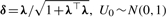, U₁~N_p(0, I_p) and the symbol ‘⊥’ indicates independence.

The multivariate skew t (MST) distribution was proposed by Azzalini and Capitaino (2003), which is related to the MSN distribution as follows:

(2)

where Z ~ SN_p(0, Σ, λ) and τ~Gamma(ν/2,ν/2). It follows from (2) that Y∣τ~SN_p(μ, Σ/τ, λ). By Proposition 1 of Lin et al. (2007), integrating out τ from the joint density of (Y, τ) yields the marginal density of Y

(3)

where t_p(·|μ, Σ, ν) denotes the pdf of p-variate t distribution with location vector μ, scale matrix Σ and degrees of freedom (df) ν∈(0,∞); T(·|ν) represents the cdf of Student's t-distribution with df ν and Δ=(Y−μ)^⊤ Σ⁻¹(Y−μ). We shall denote Y ~ ST_p(μ, Σ, λ, ν) if Y has density given in (3).

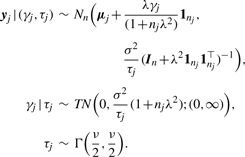
Suppose we have a set of m input profiles {y_j}_j=1^m and each response vector y_j consists of n_j consecutive observations. We assume the response vector y_j∈ℝ^n_j is generated from

where β is a p×1 vector of regression coefficients related to design matrix X_j=[x_j1…x_jnj]^T with x_jk=(x_jk1,…,x_jkp)^T; μu_j≡μ(β,x_j) is a vector-valued non-linear (differentiable) function of β governing within-profile behavior, and ε_j is the resulting error vector equal to the discrepancy between y_j and μu_j.

A skew-t based non-linear regression model is defined by assuming ε_j ~ St_nj(0,∑_j, λ_j, ν). Depending on the context, various assumptions should be made on ∑_j and λ_j to reduce the number of parameters to be estimated. Following De la Cruz (2008), we set ∑_j=σ²I_nj to reflect the assumption of exchangeable errors among individuals and λ_j=λ1_nj, where 1_nj is an n_j×1 unit vector for ensuring an identifiable model. In some circumstances, it is quite common to assume a time series like dependence structure for ∑_j, which is a function of a small number of free parameters and depends on j only through its dimension n_j. Note that the skew t can be reduced to the following particular models that enhance the ease of implementation: the skew normal (ν→∞), Student's t (λ→0) and the most common normal (λ→0; ν→∞) models.

From (2), it can be verified that

(4)

Applying Bayes' rule yields

(5)

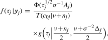(6)

where Δ_j=ε^⊤_jε_j, A_j=λ1_nj^⊤ϵ_j and c_rj=A_j[(ν+n_j+r)/(σ²ν+Δ_j)]^1/2. According to (5) and (6), it suffices to compute the following conditional expectations:

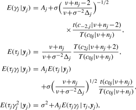(7)

where t(·|ν) is the pdf of the Student's t-distribution with df ν.

Finite mixture models are commonly used for model-based clustering (Banfield and Raftery, 1993; McLachlan and Basford, 1988). Let a curve profile be given by a sequence y_j of observations at n_j (time) points x_j and assumed to be generated by one and only one cluster (i.e. a mAb class). Then our goal is to partition {y_j}_j=1^m into g homogeneous groups (or classes). For notational convenience, let μ_ij=μ(β_i,x_j), e_ij=y_j−μ_ij, A_ij=λ_i1_nj^⊤e_ij, Δ_ij=e_ij^⊤e_ij and c_rij=A_ij[(ν_i+n_j+r)/(σ_i²ν_i+Δ_ij)]^1/2 for i=1,…,g and j=1,…,m. Define

the density of a cluster-specific skew-t non-linear regression model that relates (y_j,x_j) to θ_i=(β_i, σ_i², λ_i, ν_i).

The mixture model for profile clustering is written as:

(8)

where w_i's are mixing proportions which are constrained to be non-negative and ∑_i=1^g w_i=1 and Θ=(w₁,…,w_g−1,θ₁,…,θ_g) represents all unknown parameters. The observed data log-likelihood function of Θ is

(9)

In general, there are no explicit analytical solutions for computing the ML estimator of Θ. The EM algorithm (Dempster et al., 1977) is considered as a standard tool when applied for mixture models. In the EM framework for supporting the interpretation of incomplete data, it is convenient to introduce a set of allocation variables Z_j=(Z_1j,…,Z_gj)^T, j=1,…,m. The element Z_ij is taken to be one or zero to indicate if y_j does or does not come from the i-th component. This implies that Z_j follows a multinomial distribution with 1 trial and cell probabilities w₁,…,w_g, denoted by Z_j ~ M(1; w₁,…,w_g). Then, a hierarchical formulation of (8) obtained in conjunction with (4) is

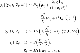(10)

Let y=(y₁,…,y_m), γ=(γ₁,…,γ_m), τ=(τ₁,…,τ_m) and Z=(Z₁,…,Z_m). It follows from (10) that the complete data log-likelihood function of Θ given (γ, τ, Z, y) is

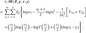(11)

where ϒ_1ij=τ_j(y_j−μ_ij)^⊤(y_j−μ_ij) and ϒ_2ij=τ_j[γ_j−λ_i1_nj^⊤(y_j−μ_ij)]².

The EM algorithm proceeds by alternately repeating the E- and M- steps where, at the k-th iteration, the E-step involves the calculation of the Q-function, which is the expected value of the complete data log-likelihood (11) conditional on y and the current estimate for Θ, is given by

(12)

To evaluate (12), the necessary conditional expectations include

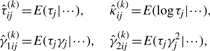(13)

where the symbol ‘|···’ stands for conditioning on Z_ij=1, y_j=y_j and and they are directly obtainable through using identities (7) and the law of iterative expectations. Moreover, we define

(14)

which is the posterior probability that the j-th curve belongs to the i-th component evaluated at the (k+1)-st iteration. Therefore, the Q-function (12) can be written as

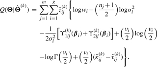(15)

where and .

In summary, the implementation of the EM algorithm proceeds as follows: E-step: given , compute , , , and , for i=1,…,g and j=1,…,n, by using Equations (13) and (14), respectively.

M-step: calculating by optimizing (15) over Θ, the updating formulae are given by

where and and are ϒ_1ij^(k)(β_i) and ϒ_2ij^(k)(β_i) in (15) with β_i replaced by . Consequently, we obtain by solving the root of the following equation:

This can be easily done with the help of the R routine ‘uniroot’. The E- and M- steps are alternately repeated until a suitable convergence rule is satisfied, e.g. the Aitken acceleration-based stopping criterion |ℓ^(k+1)−ℓ^(k+1)_∞| < ϵ, where ℓ^(k+1) is the observed log-likelihood evaluated at , ℓ^(k+1)_∞ is the asymptotic estimate of the log-likelihood at iteration k+1 (McLachlan and Krishnan, 2008; Chapter 4.9) and ϵ is the desired tolerance.

Model selection for Step 2: let X be a p-dimensional random sample drawn from a mixture distribution of g components, each with homogeneous covariance matrix Γ, and let c₁,…,c_g be a set of candidate cluster centers with c_r being the one closet to X. Sugar and James (2003) developed an alternative simple approach to identify the optimal number of clusters based on the ‘distortion function’, defined as

(16)

which is a quantity that measures the average Mahalanobis distance between X and its closest cluster center c_r. The Jump function due to Sugar and James (2003) is defined as

where C is an appropriate positive constant that makes a sharp jump at the true number of clusters and is the minimum distortion obtained by the clustering algorithms. They have proven that an appropriate number of clusters can be identified at the peak of jump based on information-theoretic ideas. Their simulation studies have also empirically shown that the Jump plot has good performance in finding the true number of clusters.

We applied the Jump function approach to the problem of curve clustering analysis. Each curve is assigned to the component with the largest posterior probability obtained by fitting model (8) for g=1,…,g_max, a pre-specified maximum number of components. We chose g_max to be 12 for all tissues, except for two (spleen and bone marrow) where the model did not converge for g > 10. Let be the fitted vector of y_j if y_j has been assigned outright to i-th cluster, say y_j∈𝒞_i. This gives

where . Then, the mean squared error for y_j∈𝒞_i is given by

which is the scaling squared distance from y_j to . It follows from (16) that the associated distortion function is empirically defined as

Theoretically, the distortion curve, versus g, is always monotone decreasing. A simple way of choosing the optimal g is to look for the point at which the magnitude of change in 's becomes negligible, especially when the subclasses are well separated. However, using the raw distortion curve could fail in certain cases. As suggested by Sugar and James (2003), the Jump plot method performs extremely well, provided that some suitable values for C are chosen. The optimal number of clusters in data can be visually determined from the peak patterns on the Jump plot. Empirical studies show that the point with largest or secondary largest jump is often the best choice.

Quality of curve clustering: to determine the quality of our clustering of mAb profiles, modeled as probability density functions, we measured mean intra- and intercluster distances using a symmetric form of Kullback–Leibler distance, denoted by sKL(p,q), between a pair of profiles (p,q), defined as follows:

where KL(p,q)=∑_tp_t log₂(p_t/q_t) at each observation point t.

To determine the quality of hierarchical clustering of mAb data, we used the R functions hclust (with Euclidean distance metric) and asw (average silhouette width). The R package ks is used for SiZer plot.

3 RESULTS

Following data preparation and preprocessing, in Step 1, mAbprofiler modeled cytometric histograms for 561 mAb samples from six tissues using skew t mixture models. Figure 1 illustrates how a profile (shown as gray curve) constructed by mAbprofiler offers a smooth and precise representation of mAb density histograms. This can be contrasted with the original cytometric input in the form of highly non-smooth patterns as shown in Supplementary Figure S1. To rigorously assess the precision of modeling with our skew t mixture models (STMIX), we computed log-likelihood maxima, BIC values, the distances D_n between the data and the fitted model (based on Kolmogorov–Smirnov test) and CPU times for STMIX as well as for two competing models of more commonly used mixtures of Gaussian (NMIX) and t distributions (TMIX), and compared them in Supplementary Table S1. Clearly, as shown by BIC, mAbprofiler gives the best fit.

In Step 2, for each tissue, mAbprofiler clustered the mAb profiles, specified as density curves, with our new algorithm for non-linear regression of skew t mixture models. It selected the model that corresponded to the optimal tissue-specific group structure using the maximal value of the Jump statistic over a range of clusters (g=1, 2…, g_max). Table 1 summarizes the results of this clustering step. The optimal choice of g over the values for which the EM converged is marked in Figure 2 and Supplementary Figure S1 (right panel). In Figure 3a–f, we show each of the six clusters of the spleen profiles. Notably, the profiles were grouped by their significant features overcoming intersample variation. Thus, the clustering was both accurate and robust. Further, Figure 3g shows the mean profile of every cluster in its own color, thereby contrasting the signature templates for every class while summarizing the characteristic features within each of them. Similar joint plots for every tissue are shown in Supplementary Figure S2, which also includes the Jump statistics that help in the determination of the optimal group structures.

Table 1.

Clustering statistics for Step 2

Tissue type	No. of samples	No. of classes	IIR	CT	gmax
Spleen	59	6	0.078	27.09	10
Thymocyte	111	12	0.068	118.04	12
Lung lavage	123	11	0.017	95.06	12
Bone marrow	48	8	0.014	23.94	10
Fetal thymus	89	12	0.038	81.24	12
Lymph node	131	8	0.072	111.21	12

For each tissue-type, its count of mAb profiles, number of profile clusters (i.e. mAb classes), IIR (average intracluster distance to average intercluster distance ratio) and computing time (CT, in minutes) of the EM algorithm for g=1,2…,g_max.

Fig. 2.

Model selection for curve clustering: maximum value of Jump for spleen indicates that 6 is the optimal number of mAb classes in that tissue.

Fig. 3.

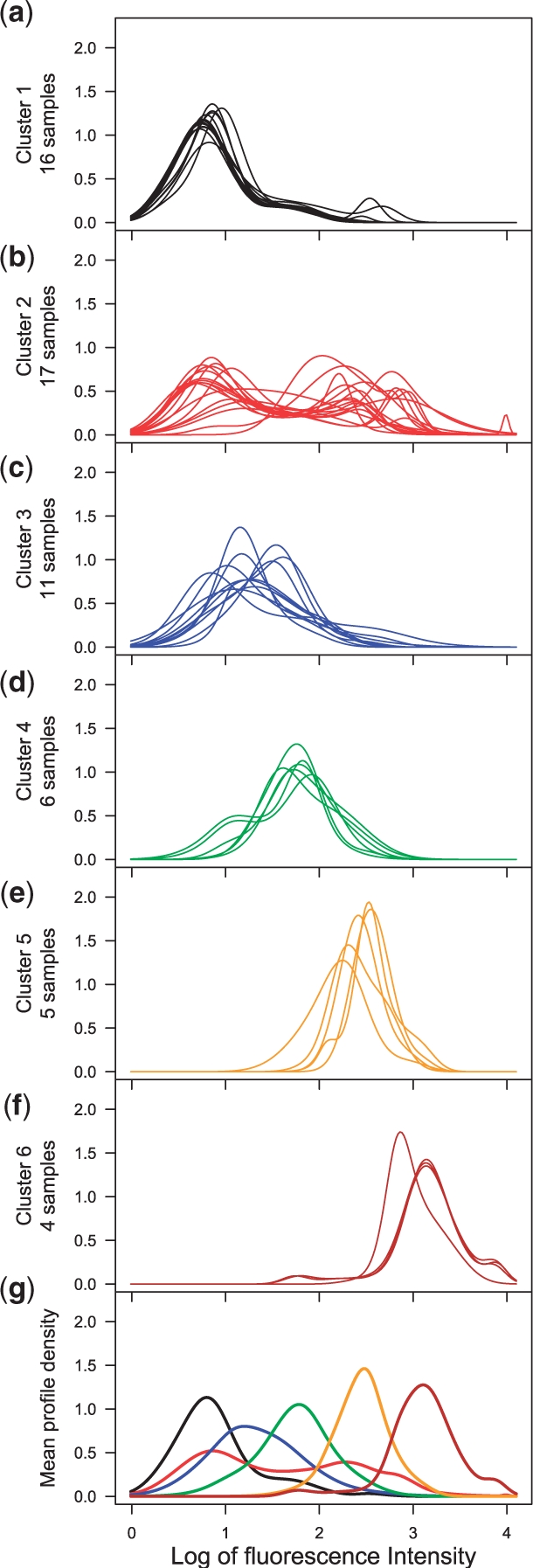
Classification of mAb profiles for spleen: in Step 2 of mAbprofiler, the profiles of all 59 mAb samples in spleen were clustered with non-linear regression of skew t mixture models. The profiles belonging to each of the six clusters (a)–(f) are shown in distinct colors. The joint plot (g) of all six mean profiles in cluster-specific colors allows visual comparison of the cluster templates.

We validated our mAb classification both computationally and empirically. Since every fitted profile is defined by a probability distribution, we computed a symmetric form of Kullback–Leibler distance (sKL) between all pairs of profiles, and observed that the average intracluster distances between profiles are considerably lower than the average intercluster distances. The ratio (IIR) in every tissue is shown in Table 1. For illustration, the distance matrix for the six clusters for spleen is shown in Supplementary Figure S3.

For empirical validation, for four tissue types (spleen, thymocytes, bone marrow and lymph node) and two classes of antibodies [class I mAb T2/39 and anti-LFA-1 mAb F10-150 as described in Pratt et al. (2009)], we generated data for two pairs of mAb such that the mAb within each pair were known to target molecules of the same class, but across pairs, they targeted molecules from distinct classes. As shown in Supplementary Figure S4, indeed all profile pairs (black thin curves) cluster together within each class (Class I in left panel or anti-LFA-1 in right panel), but separately across two distinct classes, providing experimental evidence for precise and objective classification by our framework. As in Figure 3, the mean profiles are shown in cluster-specific colors for distinguishing the two classes in each tissue.

3.1 Comparative analysis with other methods

Besides internal validation, we also compared the performance of mAbprofiler with other established methods. We began with hierarchical clustering, which is the most commonly used approach for mAb classification (Bernard and Boumsell, 1984). When we used hierarchical clustering on our mAb profiles, then the method clearly failed to capture the complex class structure and detected few clusters. Based on Average Silhouette Width (ASW), a common measure for determining the quality of hierarchical clustering, we noted that the optimal number of mAb classes according to hierarchical clustering of our data was typically restricted to four or even fewer for all tissues other than thymocytes. Moreover, little difference among the ASW scores for different number of clusters indicated that the hierarchical clusters had low separation (Supplementary Figure S5).

Thereafter, we adopted the established protocol of Pratt et al. (2009) in which mAb histograms were first smoothed with SiZer, and then hierarchical clustering was performed with those smoothed profiles. We show the results of that approach on our data using SiZer plots for the different tissues in Supplementary Figure S6a–f. As depicted with the dendrograms, while the larger clustering structures were detected with smoothing, the finer structures were often ignored, thus resulting in highly heterogeneous classes. This can be seen clearly in the largest clusters in spleen, lung lavage and bone marrow.

Finally, we also studied a combination of our approach with that of Pratt et al. (2009) in which we clustered the SiZer-smoothed profiles (i.e. we replaced Step 1 of mAbprofiler) using our NLRST algorithm (i.e. we retained Step 2 of mAbprofiler). We observed that while NLRST could identify more classes in the same SiZer profiles for some tissues, the overall gain was not significant. In other words, the fact that mAbprofiler identified a much richer class structure could be attributed to the dual contributions of both Steps 1 as well as 2 of the new framework. While NLRST tackles the intersample variation along x-direction (feature location), the skew t mixture pdf provides a precise and continuous representation of the y-direction (feature significance). The resulting effectiveness of mAbprofiler's two-step approach is illustrated, for example, in the eight class-templates for the lymph node which are distinctive along both x- and y-directions (Supplementary Figure S2, left panel bottom plot). In contrast, the other methods failed to capture that dual complexity and identified only few dominant clusters. The full comparison of classes detected by all four methods is shown in Supplementary Table S2.

4 DISCUSSION

Monoclonal antibodies play an immensely important role in molecular biology, biochemistry and medicine. Their utility for probing, stimulating or inhibiting specific target molecules supports numerous diagnostic and immunotherapeutic applications (Zola, 2006). Further, design and development of new mAbs are also of great industrial significance. Therefore, objective mAb classification is essential for categorizing and comparing the known as well as the newly developed mAb panels. Besides biochemical methods like immunoprecipitation, this is achieved by clustering flow cytometric reactivity patterns of mAb in different cell types. Unlike traditional HLDA workshops which classified leukocyte surface (CD) molecules (Zola and Swart, 2005) using cell lines, Pratt et al. (2009) recently described a system to facilitate practical mAb characterization in animal tissues. This approach is consistent with the new human cell differentiation molecules (HCDM) focus on various non-hematopoeitic cell types (Zola, 2006). In the present study, we enhanced that approach further by (i) generating a new, larger and more varied collection of mAb patterns in six different tissues, and importantly, by (ii) constructing a new analytical framework, mAbprofiler, to formally address the technical challenges of mAb characterization. Our two-step framework provides precise profiling of cytometric histograms (Step 1) followed by novel clustering of these curve profiles (Step 2). In addition to characterizing mAb for the present study, mAbprofiler can also provide a general framework to allow users to search for archived class signatures or to construct and classify new mAb profiles in a systematic way.

Previous mAb classification studies (e.g. Pratt et al., 2009; Salganik et al. 2005) have used non-parametric kernel density estimation techniques for detection of significant features in cytometric histograms, typically followed by hierarchical clustering based on Euclidean distances between the features. While being practical, such approaches may not always be precise or robust. For instance, the accuracy of density estimates by kernel-based methods are known to be strongly influenced by bandwidth selection (Jones et al., 1996). As observed in Supplementary Figure S1, significance of the peak features in a given sample, as detected by the program SiZer, is clearly dependent on the choice of bandwidth. This poses a key practical problem, especially since we seek to do unsupervised classification of new mAb profiles. While recent advances in kernel-based techniques have addressed different aspects of cytometric analysis (e.g. Duong et al., 2009; Naumann et al., 2010), we followed the parametric approach developed by Pyne et al. (2009) and (Frühwirth-Schnatter and Pyne, 2010), which uses finite mixtures of skewed t distributions, for our purposes. Observations of non-Gaussian features in cytometric data made by these and other recent studies (Ho et al., 2011; Lo et al., 2008; Pyne et al., 2011) led us to use this more general parametric family of distributions, which also the includes Gaussian distribution as a special case.

Finite mixture models have been extensively used in biology and medicine (Frühwirth-Schnatter, 2006; McLachlan and Peel, 2000). In Step 1 of mAbprofiler, we presented a univariate version of the Pyne et al.'s (2009) approach for profiling asymmetric and noisy mAb patterns with finite mixture model of skew t distributions fit via our own EM algorithm (see Supplementary Material). The EM algorithm converges fast in practice, and supports multiple well-known model selection criteria such as AIC, BIC and ICL. In the resulting smooth and precise profiles (see illustrative sample in Fig. 1), every component is specified by rigorous model parameters such as location, size, shape, variance and degrees of freedom. Further, the parametric design enables mAbprofiler to specify the significance of every mAb feature with a smooth and continuous probability density function, which can be represented as a curve that is well defined at any resolution. Importantly, in Step 2, mAbprofiler's non-linear regression of skew t mixture models can cluster these curve profiles accurately for every cell type. While Step 1 follows the approach of (Pyne et al., 2009), Step 2 introduces novel methodology and the EM algorithm implementing it.

A key challenge for cytometric data analysis is intersample variation. Similar mAb profiles can vary considerably in both their significance and location, which must be addressed by any algorithm designed for classifying cytometric data. While it is possible to transform or shift and align the data (e.g. Hahne et al., 2010; Lo et al., 2008), we want to cluster the mAb profiles precisely in terms of the distinctive features that they present as curves with a robust approach. To systematically model that intersample variation, in Step 2, mAbprofiler presented a new non-linear regression algorithm. It is also a solution for the more generic problem of curve clustering, an important topic in the field of pattern recognition which has not received much attention in the past (e.g. Gaffney, 2004; Gaffney et al., 2007; Liu and Yang, 2009). Here we extended the work of Gaffney (2004) and Jones and McLachlan (1992) to introduce non-linear regression of skew t mixture models for robust curve clustering with asymmetric variation among the curve features. In our comparative analysis with other methods, we observed that hierarchical clustering is not as well suited for such clustering probably because it critically relies on precise pairwise distances between points. Trying to reduce a curve profile to a point–albeit a multidimensional point—can lead to loss of information about features due to binning of the data as specified by a cytometric histogram. That leads to fewer and less well-separated hierarchical clusters, as illustrated in Supplementary Figure S5.

The problem of using hierarchical clustering for mAb classification gets further compounded with the issue of bandwidth selection in smoothing of cytometric histograms such as in the protocol of Pratt et al. (2009). For our data, the SiZer-smoothed features for a predetermined bandwidth led to mAb classes with high heterogeneity. While our NLRST (Step 2) clustering could improve detection of the classes with the same SiZer profiles, the net gain was not significant. Therefore, the identification of a much richer group structure by mAbprofiler, as shown in Supplementary Table S2 (and the class templates in Fig. 3g and Supplementary Figure S2, left panel) may be attributed to the dual advantage of both Steps 1 and 2 of the new framework. Hierarchical clustering fails to capture the complexity of data when presented in the form of noisy curve profiles in which the true significance of features is not apparent. This is even more difficult if there are few significant features, which, in turn, might suffer from intersample variation. By addressing these issues, mAbprofiler produced robust mAb classes—specified as curves of probability density functions—even in the presence of non-Gaussian variation. It achieves this without any need for transforming the profiles or reducing them to points as required for hierarchical clustering.

The new framework has several additional advantages. Its use of Jump statistic provides a suitable criterion for optimal model selection in profile clustering. Each step of mAbprofiler can be performed independently with its own EM algorithm, which offers the flexibility of pipelining the framework with external algorithms. As output, not only does mAbprofiler produce a smooth profile for a mAb histogram, it also generates a mean template for the ‘signature’ pattern of every mAb class, along with parametric description of significant features therein. As a result, class templates can be archived, and later searched for information on overall or specific characteristics of such known mAb classes. Thus, it facilitates pattern matching with newly constructed mAb profiles, which can be grouped with classes having the most similar templates. Our computational and empirical validation of mAbprofiler classification shows how this is achieved. Another feature of our approach is that it does not require a clonal population. Expression can be analyzed both on individual cells and within a complex cell population. Moreover, our non-Gaussian model can be easily extended to temporal mAb profiling (Pyne et al., 2011), e.g. for measurements over the course of dampening of an inflammation in a certain tissue. The strength of mAbprofiler lies in providing a much-needed robust and objective framework for mAb characterization in different cell types and tissues.

Funding: TL thanks the National Science Council of Taiwan (NSC99-2118-M-005-001-MY2) for financial support.

Conflict of Interest: none declared.

REFERENCES

- Arellano-Valle R.B., et al. Skew-normal linear mixed models. J. Data Sci. 2005;3:415–438. [Google Scholar]
- Azzalini A., Capitaino A. Distributions generated by perturbation of symmetry with emphasis on a multivariate skewtdistribution. J. R. Stat. Soc. Ser. B. 2003;65:367–389. [Google Scholar]
- Azzalini A., Dalla-Valle A. The multivariate skew-normal distribution. Biometrika. 1996;83:715–726. [Google Scholar]
- Banfield J.D., Raftery A.E. Model-based Gaussian and non-Gaussian clustering. Biometrics. 1993;49:803–821. [Google Scholar]
- Bernard A., Boumsell L. The clusters of differentiation (CD) defined by the first international workshop on human leucocyte differentiation antigens. Hum. Immunol. 1984;11:1–10. doi: 10.1016/0198-8859(84)90051-x. [DOI] [PubMed] [Google Scholar]
- De la Cruz,R. Bayesian non-linear regression models with skew-elliptical errors: applications to the classification of longitudinal profiles. Comput. Stat. Data Anal. 2008;53:436–449. [Google Scholar]
- Dempster A.P., et al. Maximum likelihood from incomplete data via the EM algorithm (with discussion) J. R. Stat. Soc. Ser. B. 1977;39:1–38. [Google Scholar]
- Duong T., et al. Highest density difference region estimation with application to flow cytometric data. Biom. J. 2009;51:504–521. doi: 10.1002/bimj.200800201. [DOI] [PubMed] [Google Scholar]
- Frühwirth-Schnatter S. Finite Mixture and Markov Switching Models. New York: Springer; 2006. [Google Scholar]
- Frühwirth-Schnatter S., Pyne S. Bayesian inference for finite mixtures of univariate and multivariate skew normal and Skew-tdistributions. Biostatistics. 2010;11:317–336. doi: 10.1093/biostatistics/kxp062. [DOI] [PubMed] [Google Scholar]
- Gaffney S. PhD Dissertation. Irvine: Department of Computer Science, University of California; 2004. Probabilistic curve-aligned clustering and prediction with mixture models. [Google Scholar]
- Gaffney S.J., et al. Probabilistic clustering of extratropical cyclones using regression mixture models. Clim. Dynam. 2007;29:423–440. [Google Scholar]
- Gilks W.R., Shaw S. Statistical analysis. In: Schlossman S., et al., editors. Leucocyte Typing V. Oxford: Oxford University Press; 1995. pp. 8–13. [Google Scholar]
- Hahne F., et al. Per-channel basis normalization methods for flow cytometry data. Cytometry Part A. 2010;77:121–131. doi: 10.1002/cyto.a.20823. [DOI] [PMC free article] [PubMed] [Google Scholar]
- Herzenberg L.A., et al. Monoclonal antibodies and the FACS: complementary tools for immunobiology and medicine. Immunol. Today. 2000;21:383–390. doi: 10.1016/s0167-5699(00)01678-9. [DOI] [PubMed] [Google Scholar]
- Ho H.J., et al. Maximum likelihood inference for mixtures of skew Student-t-normal distributions through practical EM-type algorithms. Stat. Comput. 2011 doi: 10.1007/s11222-010-9225-9. [Google Scholar]
- Jones P.N., McLachlan G.J. Fitting finite mixture models in a regression context. Aust. J. Stat. 1992;34:233–240. [Google Scholar]
- Jones M.C., et al. A brief survey of bandwidth selection for density estimation. J. Am. Stat. Assoc. 1996;91:401–407. [Google Scholar]
- Kim E.Y., et al. Using a neural network with flow cytometry histograms to recognize cell surface protein binding patterns. Proc. AMIA Symp. 2002:380–384. [PMC free article] [PubMed] [Google Scholar]
- Li X., et al. Hybridoma screening using an amplified fluorescence microassay to quantify immunoglobulin concentration. Hybridoma. 1995;14:75–78. doi: 10.1089/hyb.1995.14.75. [DOI] [PubMed] [Google Scholar]
- Lin T.I., et al. Robust mixture modeling using the skewtdistribution. Stat. Comput. 2007;17:81–92. [Google Scholar]
- Liu X., Yang M.C.K. Simultaneous curve registration and clustering for functional data. Comput. Stat. Data Anal. 2009;53:1361–1376. [Google Scholar]
- Lo K., et al. Automated gating of flow cytometry data via robust model-based clustering. Cytometry Part A. 2008;73:321–332. doi: 10.1002/cyto.a.20531. [DOI] [PubMed] [Google Scholar]
- McLachlan G.J., Basford K.E. Mixture Models: Inference and Application to Clustering. New York: Marcel Dekker; 1988. [Google Scholar]
- McLachlan G.J., Krishnan T. The EM Algorithm and Extensions. 2. New York: John Wiley & Sons; 2008. [Google Scholar]
- McLachlan G.J., Peel D. Finite Mixture Models. New York: Wiley; 2000. [Google Scholar]
- Naumann U., et al. The curvHDR method for gating flow cytometry samples. BMC Bioinformatics. 2010;11:44. doi: 10.1186/1471-2105-11-44. [DOI] [PMC free article] [PubMed] [Google Scholar]
- Pratt J.P., et al. Hierarchical clustering of monoclonal antibody reactivity patterns in nonhuman species. Cytometry. Part A. 2009;75:734–742. doi: 10.1002/cyto.a.20768. [DOI] [PMC free article] [PubMed] [Google Scholar]
- Pyne S., et al. Automated high-dimensional flow cytometric data analysis. Proc. Natl Acad. Sci. USA. 2009;106:8519–8524. doi: 10.1073/pnas.0903028106. [DOI] [PMC free article] [PubMed] [Google Scholar]
- Pyne S., et al. Proceedings of IEEE 1st International Conference on Computational Advances in Bio and Medical Sciences (ICCABS) Institute of Electrical and Electronics Engineers (IEEE); 2011. Parametric modeling of cellular state transitions as measured with flow cytometry; pp. 147–152. [Google Scholar]
- Salganik M.P., et al. Classifying antibodies using flow cytometry data: class prediction and class discovery. Biomet. J. 2005;91:785–800. doi: 10.1002/bimj.200310142. [DOI] [PubMed] [Google Scholar]
- Spiegelhalter D.J., Gilks W.R. Statistical analysis. In: McMichael A.J., et al., editors. Leucocyte Typing I. Oxford: Oxford University Press; 1987. pp. 14–24. [Google Scholar]
- Sugar C.A., James G.M. Finding the number of clusters in a dataset: an information-theoretic approach. J. Am. Stat. Assoc. 2003;98:750–763. [Google Scholar]
- Zeng Q., et al. Proceedings of the AMIA Symposium. American Medical Informatics Association (AMIA); 2002. Matching of flow-cytometry histograms using information theory in feature space; pp. 929–933. [PMC free article] [PubMed] [Google Scholar]
- Zeng Q.T., et al. Feature-guided clustering of multi-dimensional flow cytometry datasets. J. Biomed. Informat. 2007;40:325–331. doi: 10.1016/j.jbi.2006.06.005. [DOI] [PubMed] [Google Scholar]
- Zola H. Medical applications of leukocyte surface molecules–the CD molecules. Mol. Med. 2006;12:312–316. doi: 10.2119/2006-00081.Zola. [DOI] [PMC free article] [PubMed] [Google Scholar]
- Zola H., Swart B. The human leucocyte differentiation antigens (HLDA) workshops: the evolving role of antibodies in research, diagnosis and therapy. Cell Res. 2005;15:691–694. doi: 10.1038/sj.cr.7290338. [DOI] [PubMed] [Google Scholar]