Abstract
The apparent diffusion coefficient (ADC) derived from diffusion-weighted imaging (DWI) correlates inversely with tumor proliferation rates. High-grade gliomas are typically heterogeneous and the delineation of areas of high and low proliferation is impeded by partial volume effects and blurred borders. Commonly used manual delineation is further impeded by potential overlap with cerebrospinal fluid and necrosis. Here we present an algorithm to reproducibly delineate and probabilistically quantify the ADC in areas of high and low proliferation in heterogeneous gliomas, resulting in a reproducible quantification in regions of tissue inhomogeneity. We used an expectation maximization (EM) clustering algorithm, applied on a Gaussian mixture model, consisting of pure superpositions of Gaussian distributions. Soundness and reproducibility of this approach were evaluated in 10 patients with glioma. High- and low-proliferating areas found using the clustering correspond well with conservative regions of interest drawn using all available imaging data. Systematic placement of model initialization seeds shows good reproducibility of the method. Moreover, we illustrate an automatic initialization approach that completely removes user-induced variability. In conclusion, we present a rapid, reproducible and automatic method to separate and quantify heterogeneous regions in gliomas.
Keywords: Diffusion imaging, expectation maximization, heterogeneity, glioma
Introduction
Diffusion-weighted imaging (DWI) has been extensively used as an imaging method that yields surrogate parameters for tumor cellularity and proliferation and may be used to monitor treatment response in the brain and the abdomen[1–4]. The apparent diffusion coefficient (ADC) value depicts the average diffusion or the Brownian molecular motion of water within a voxel[3,4]. A low ADC correlates, among many other factors, with a high cellular density and increased proliferation, whereas a high ADC is related to low cellular density and low proliferation[1,2,5].
Since quantitative measures of the ADC in tumor regions may be of great clinical importance both in initial tumor grading as well as for therapy follow-up, such measures must be extracted from the data in a reproducible fashion. Commonly, DWI data are evaluated using manual region of interest (ROI) analysis. Using such analysis, a negative correlation between the ADC and the micro vessel density, as a marker of tumor proliferation was found in the tumor bulk[6]. In another study, the minimum ADC in astrocytic tumors (all WHO Grades I–IV) was found to be in general negatively correlated to the Ki-67 labeling index (LI), which is an index for cell proliferation[7]. However, since the borders within heterogeneous tumor regions on the one hand, and between cerebrospinal fluid (CSF) and necrotic areas on the other hand, are ill defined, the ROI placement is inherently user dependent. Thus, an objective automated method for tissue segmentation beyond manual ROI placement is needed to enable a reliable ADC quantification in heterogeneous gliomas.
Whereas previously proposed methods such as region growing, live wire or shape-based segmentation require and produce sharp boundaries, statistical segmentation approaches are more suitable to incorporate soft boundaries by yielding class probabilities. Gaussian mixture models with the help of expectation maximization (EM) optimization[8–10] or similar optimization strategies are one approach to achieve a probabilistic classification based on histogram analysis[11–16].
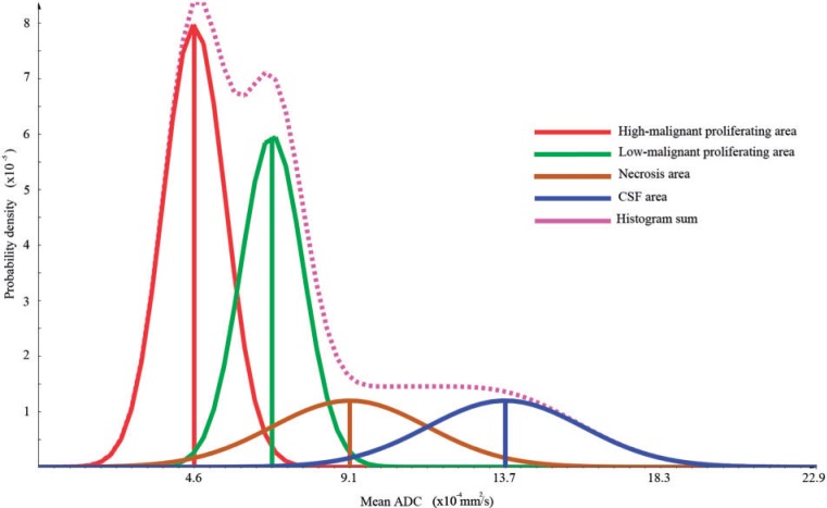
An important first requirement for statistical segmentation approaches is that the distributions of the measurement value (e.g. the ADC) within the expected different segments (e.g. high vs low cellularity) can be separated into a superposition of 2 Gaussians. If this is given for the tumor volume, the probability can be calculated that this voxel belongs to one of the expected clusters. In Fig. 1, we illustrate a theoretical distribution of the ADC in a tumor region in the brain.
Figure 1.
Theoretical histogram: red depicts the high-proliferating area, green the low-proliferating region, brown the necrosis area and blue the CSF. The volume fractions of the different compartments were set to 0.4:0.3:0.15:0.15 for high-proliferating, low-proliferating, necrosis, and CSF, respectively.
Based on these individual probabilities, using the EM approach[8–10], the assumed tissue groups can be found. The overall probability of the found cluster, which can be seen as a quality measurement of the complete approach, is then given by the so-called posterior probability. Furthermore, the given probabilities within the tumor area can be used to take partial volume effects into account[11–13]. These likelihoods can be used to come to a probabilistic quantification that allows for a reproducible quantification in regions of tissue inhomogeneity[11,12]. The probabilistic quantification does not necessarily ensure a more valid delineation. However, the objectivity of the quantification increases by applying probabilistic assumptions.
In this article, we describe a method to objectively separate high-proliferating from low-proliferating parts in heterogeneous gliomas represented in diffusion-weighted images. We evaluate the plausibility and the reproducibility of the implemented approach that includes multimodal image overlay, signal intensity thresholding and probabilistic ADC-based clustering.
Materials and methods
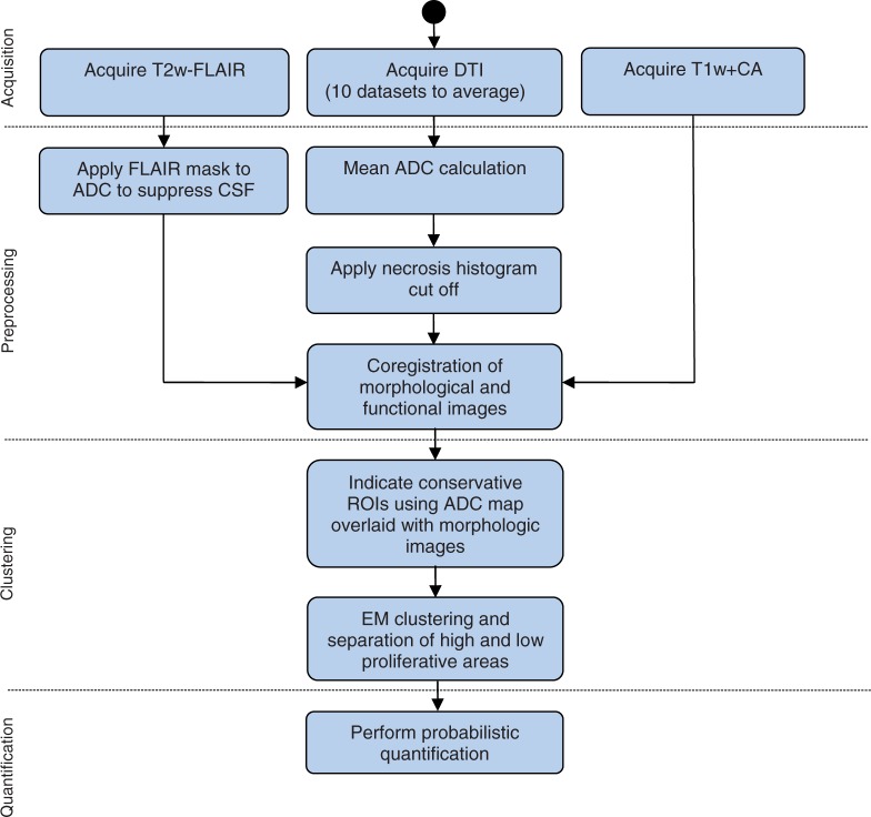
Ten patients, 8 males and 2 females, with histologically proven grade III–IV glioma were included in the study. The group consisted of 2 grade III and 8 grade IV patients; the mean age was 69 ± 14 years. Patient names were rendered anonymous and the resulting code used to uniquely link data and patient. Diffusion tensor imaging (DTI), axial T2-weighted fluid attenuated inversion recovery (FLAIR), and contrast-enhanced T1-weighted magnetic resonance imaging (MRI) data were acquired and processed in order to obtain a quantification of ADC in high and low malignant tissue. The extent of the gross tumor volume (GTV) was delineated manually by a radiologist on the T2-weighted FLAIR data. T1-weighted contrast-enhanced imaging was used for delineation of the high-proliferating area within the GTV. Fig. 2 gives an overview of the steps performed during the analysis.
Figure 2.
Overview of the processing steps from image acquisition to quantification. CSF, cerebrospinal fluid; CA, contrast agent; EM, expectation maximization.
Imaging parameters
Measurements were performed on a 1.5-T whole-body clinical MRI scanner equipped with a quadrature head coil (Magnetom Symphony, Siemens Healthcare, Erlangen, Germany, gradient strength = 40 mT/m).
DTI
Fifty axial slices were acquired; using a thickness of 2.5 mm, 6 gradient directions, 2 b-values (0 and 1000 s/mm2) and 10 averages. Repetition time (TR)/echo time (TE) 8400/108; voxel size 2.5 mm3; resolution 96 × 96; field of view 240 × 240 mm2.
T2-weighted FLAIR
Twenty-four axial slices; TR/TE 9000/114; voxel size 0.5 × 0.5 × 5.0 mm3; resolution 448 × 512; field of view 210.11 × 210.11 mm2; inversion time 2500; slice thickness of 5 mm.
T1-weighted contrast-enhanced imaging
Twenty-four axial slices; TR/TE 700/18; voxel size 0.5 × 0.5 × 5.0 mm3; resolution 512 × 512; field of view 240.13 × 240.13 mm2.
ADC calculation
Post-processing was performed using the MeVisLab development environment (Fraunhofer MEVIS, Bremen, Germany). The tensor components were estimated by linear least squares calculation. The ADC is determined by the following equation:
| (1) |
where λi is the ith eigenvalue of the tensor.
Preprocessing
To improve the signal to noise ratio of the diffusion data, the 10 averages were matched spatially using a linear registration model, normalized cross-correlation as a similarity measure, and trilinear interpolation. To further improve the matching, we re-sampled the data to a finer grid of an isotropic voxel size of 1.25 mm using a cubic B-spline for the interpolation.
The axial T1-weighted contrast-enhanced images as well as the T2-weighted FLAIR images were registered onto the ADC map using normalized mutual information and trilinear interpolation.
Exclusion of CSF and necrosis
CSF is clearly hypointense in T2-weighted FLAIR images and a mask was created in the corresponding images to exclude the voxels belonging to the lower quantile in the T2-weighted FLAIR histogram. Similarly, an ADC threshold >0.001 mm2/s was used to exclude necrotic areas.
Manual placement of conservative ROIs
To obtain reference ADC values for high- and low-proliferative areas, a radiologist manually placed conservative ROIs in regions that clearly represented one of the two classes. All 3 acquired MRI datasets were taken into account.
Test for gaussianity
To justify the later use of a Gaussian mixture model for automated clustering of the 2 regions, a χ2 test was performed on the ADC distributions using ROOT (CERN, Switzerland).
Probabilistic segmentation
The probabilistic segmentation was performed by fitting a mixture model of 2 Gaussians to the normalized histogram within the masked GTV using the EM algorithm. The EM clustering with Gaussian mixture models is described in further detail in Refs.[8,9]. The derived posterior probabilities of the segmented voxels were used to quantify the ADC of the low- and high-proliferative regions by calculating the weighted sum by the posterior probability of the corresponding ADC measures.
Manual initialization of the model
To manually initialize the EM algorithm, the starting parameters were derived from the manually drawn ROIs. The stability of the approach with regard to the initialization was assessed by systematically choosing ADC values from the ROIs as class means. This procedure was repeated 10 times. The ADC from the conservative ROIs was averaged and the mean of the maximum values of the high-proliferating ROIs +σ and the mean of the minimum values of the low-proliferating ROIs −σ were used as a criterion to exclude runaway values in this test. To evaluate the reproducibility, dot plots were generated and intra-class coefficients (ICCs) were calculated from 10 initializations from all 10 patients using the software Stata (College Station Release 11; StataCorp LP, TX, USA).
Automated initialization of the model
In order to automatically initialize the EM algorithm, the fully automated model initialization as given in Ref.[13] was implemented. The GTV describes the gross tumor volume, K is the number of clusters, μk is the mean, σk is the variance and πk is the fraction of cluster k belonging to the whole Gaussian mixture model (Eq. (5)).
| (2) |
| (3) |
| (4) |
| (5) |
To evaluate the plausibility of the automated clustering, the ADC in both regions found using the automated approach was compared with the value from the seed-based initialization. The results were included in the dot plots mentioned above. Further details on the EM clustering approach are given in the Appendix.
Results
Analysis of the manually placed ROIs
The ADC distributions within the conservative ROIs with absolute frequency were averaged and showed 2 distinct peaks in all patients (see Fig. 3). The χ2 test yields the following parameters:
High-proliferating tissue χ2 (0.95; 100−3 = 97) = 121.0 > 89.2
Low-proliferating tissue χ2 (0.95; 100−3 = 97) = 121.0 > 85.9
Figure 3.
Original averaged full frequency histograms consisting of conservative areas. The high-proliferating area is highlighted in red and the low-proliferating area is shown in green. The Gaussian curve fits the area displayed (dashed curves).
The following absolute ADC values were found by averaging over all patients:
High-proliferating tissue 4.13 × 10⁻⁴ ± 9.1 × 10⁻⁵ mm2/s
Low-proliferating tissue 7.26 × 10⁻⁴ ± 9.9 × 10⁻⁵ mm2/s
Histogram clustering results
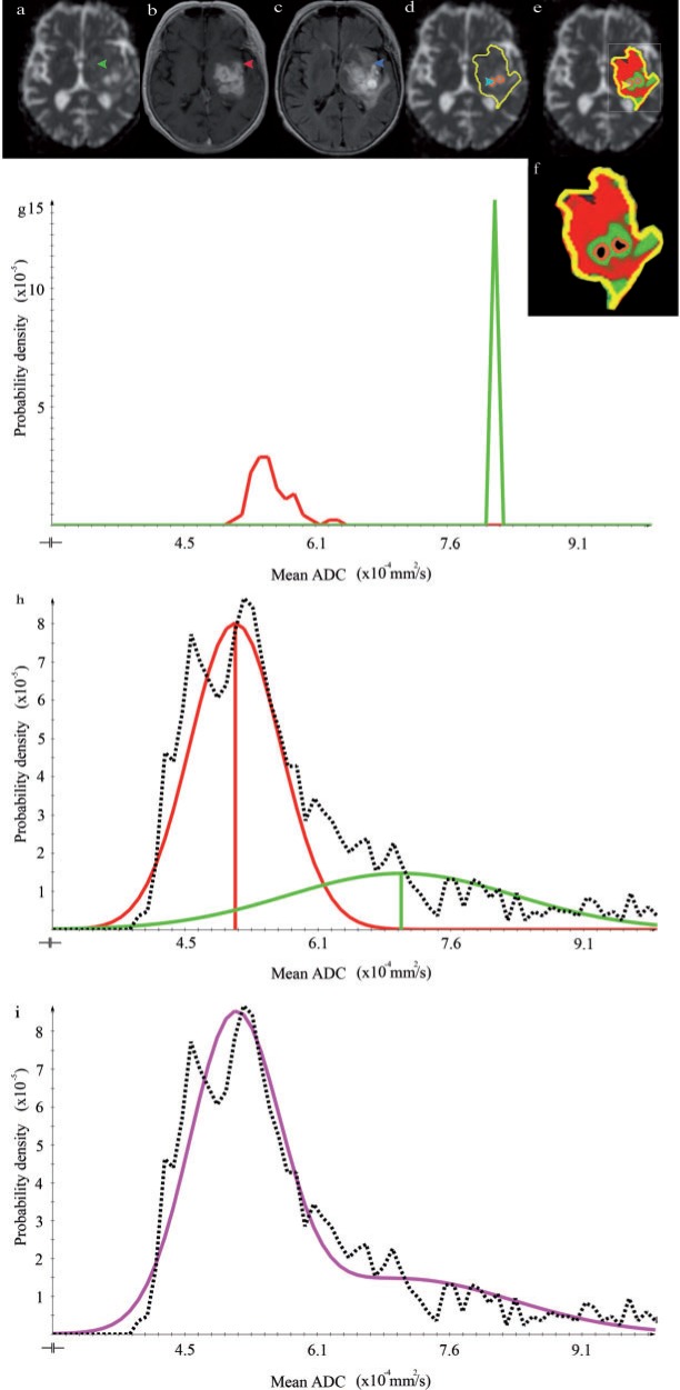
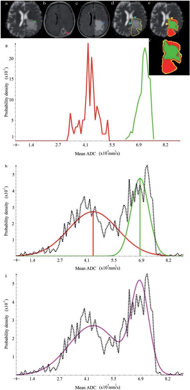
The Gaussian mixture model appropriately represented the histogram of the ADC values in the GTV in all 10 patients. This is exemplarily shown on 3 patients in Figs. 4i, 5i and 6i. The class ADC values found using the clustering method corresponded well with the mean ADC values in the manually drawn ROIs (compare (f) and (g) in Figs. 4–6). Qualitatively, the found ADC distributions (purple lines) correspond well to the theoretically introduced model shown in Fig. 1.
Figure 4.
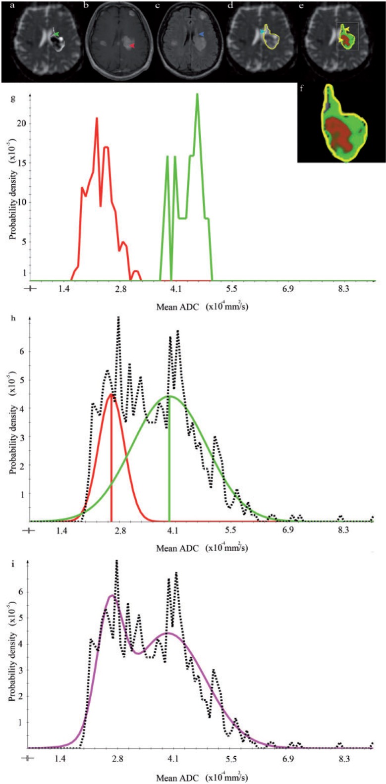
Imaging data, histogram analysis, and resulting segmentation of patient 1 (WH) (a) Axial ADC map. The arrow points to a low-proliferative area of the tumor. (b) Axial contrast-enhanced T1-weighted image. The arrow indicates a high-proliferating part of the tumor. (c) Axial T2-weighted FLAIR image. The arrow points to a low-proliferative area of the tumor. (d) ADC map with GTV outlined in yellow. The arrow indicates CSF. (e) Segmentation result shows the posterior probability of high- (red) and low-proliferative (green) areas. (f) Enlarged outline of the posterior probability as shown in (e). (g) ADC histogram within the manually drawn ROIs. High- and low-proliferating distributions are represented in red and green, respectively. (h, i) ADC distribution within the GTV. The dotted line shows the ADC distribution after necrosis and CSF exclusion. The fitted Gaussian distributions for the high- and low-proliferating tissue classes are depicted in red and green, respectively. The sum of these distributions represents the data appropriately (see purple line).
Figure 5.
The results for patient 2 (SH) organized as in Fig. 4. An interesting aspect in this patient is the almost complete lack of clearly definable low malignant areas. This can be appreciated by comparing the large size of the contrast-enhancing area in (b, arrow) with the hyperintense T2-weighted FLAIR area of similar size (c, arrow). The central necrotic areas of the tumor are outlined in (d, arrow and outlines). In the resulting segmentation (e), these areas are excluded due to the necrosis cut-off. The overall clustering result is plausible since mainly high malignant areas are found. Only some of the partial volume between necrosis and high-proliferative areas (e, arrow) is misclassified as low proliferating. The sum of the Gaussian distributions represents the data appropriately (i, purple line).
Figure 6.
The results for patient 3 (SHE) organized as in Fig. 4. The GTV outline in this patient includes normal brain tissue (d, arrows). This leads to a misclassification of normal brain tissue as a high-proliferative area (e, arrows). The sum of the Gaussian distributions represents the data appropriately (h, purple line).
Fig. 4 demonstrates the successful use of the CSF suppression, yielding a good separation of CSF and low-proliferative areas using the T2-weighted FLAIR cut-off. Fig. 5 similarly demonstrates the usefulness of the ADC-based necrosis cut-off. Note, however, that in the border region between necrosis and high-proliferative areas, a small region of misclassification occurred (Fig. 5e, arrows). Fig. 6 again demonstrates that high- and low-proliferative areas could be separated appropriately. However, it also shows a potential pitfall in cases where the GTV includes healthy brain tissue that is erroneously classified as high malignant (Fig. 6e).
Reproducibility and automated segmentation
For all 10 patients, the clustering routine was repeated 10 times using representative initialization seed voxels (Fig. 7). Each segmentation took only 0.1 s and thus, is virtually a real-time approach. For the low- and high-proliferative area, ICCs of 0.920 and 0.996 were found, respectively, indicating good agreement[3]. The automated clustering results are within the range of results found using the seed-based initialization and are indicated as gray crosses. The automated clustering was successful in all 10 cases.
Figure 7.
Dot plots of the clustering results using conservative ROIs and automated clustering. (a) Results of the seed point segmentation within the high-proliferating region (black dots) and automated segmentation (black crosses). Fractional outliers were found in BM 4/10 and in JA 1/10. The ICC for the seed-based initialization was 0.92. Note that the ADC from the automated clustering is well within the range of the seed point-based measurement. (b) Results of the seed point segmentation within the low-proliferating region. No complete outliers were found. Fractional outliers were found in BM 4/10, WF 1/10. The ICC for the seed-based initialization was 0.996. Again note that the ADC from the automated clustering is well within the range of the seed point-based measurement.
Discussion
In this work, we show that low- and high-proliferating areas in high-grade gliomas can be objectively delineated and probabilistically quantified by an EM algorithm. We propose an automated and rapid approach that anticipates the heterogeneous nature of high-grade gliomas. The application of a Gaussian mixture model is validated by a χ2 test of the averaged high-proliferating and low-proliferating ROIs, yielding Gaussian distributions in the different areas.
Quantitatively, we demonstrate that the derived mean values of this theoretical model are plausible. Through the application of a statistical algorithm with a Gaussian mixture model, we are able to probabilistically quantify the ADC in areas of low- and high-proliferation in high-grade gliomas. This unsupervised algorithm is plausible because the overall distribution fits well to the raw data and the found clusters correspond well to the conservative ROIs. The high ICCs indicate a good reproducibility of the clustering approach. Furthermore, automated clustering was successful in all 10 patients.
By application of a binary T2-weighted FLAIR mask, CSF could be excluded robustly (Fig. 4). Necrotic areas could be suppressed by application of an ADC-based histogram cut-off. However, the necrosis threshold is not completely satisfactory because it cannot suppress necrosis totally without additionally cutting off apparent low-proliferating tumor tissue (Fig. 5).
Limitations
A limitation of our current approach is that the signal overlap between normal tissue and high-proliferating areas[17] is not solved. Potentially, the addition of a partial volume class may mitigate this error. A further, related limitation is that the method only clusters on a predefined GTV drawn on a two-dimensional slice. Future research should extend the method onto the whole brain, resulting in a fully automated three-dimensional whole-brain clustering algorithm that includes and defines contextual three-dimensional constraints. Another limitation of our study was that no biopsies from different tumor regions could be obtained. Thus, we can only rely on the available image data and the unique ADC distribution to obtain a plausible separation of high- and low-proliferative areas.
The resulting problems of intensity overlap as discussed above and the definition of three-dimensional constraints may be addressed by incorporation of algorithms that include prior knowledge of spatial and anatomical constraints of normal anatomy and tumor tissue[14,18]. In these publications, a discriminative variant of the usually generative Markov random fields in combination with a support vector machines (SVM) algorithm was used, which may be combined with the approach proposed here.
A potential drawback of the EM algorithm may be data overfitting[8]. Although deterministic, the algorithm may converge towards a local maximum in the log-likelihood step. This is due to singularities that can occur if one mean of the Gaussian mixture model μk equals xn which denotes an observed data point. In this case, the log-likelihood term goes to infinity and thus has to be excluded from the maximization procedure and only a local maximum can be achieved. However, in our case, we did not encounter these potential difficulties regarding the objectivity of the retrieved ADC values, considering the applied test. In Ref.[19] several EM techniques were evaluated for brain segmentation to overcome singularities and compared with underlying ground truth. A variational EM algorithm and 2 hybrid approaches, using genetic algorithms in combination with EM and the variational approach plus genetic algorithms, respectively, were evaluated. In Ref.[20], it can be clearly seen that the simple hybrid algorithm (GA plus EM) outperforms the classic EM algorithm in terms of a higher log-likelihood result and moreover a faster convergence at equal computational costs. In Ref.[19], the hybrid variational approach in conjunction with EM outperforms all other proposed algorithms. Regarding complexity pertaining to the variational approach, Ref.[8] describes a little complexional overhead.
Thus, the proposed variational approach in combination with genetic algorithms may improve objective parameter estimation, also in our setting. Future research should explore this combined approach.
Future research and practical applications
The probabilistic ADC measurement in gliomas as proposed here can be used for the planning of resections and biopsies, as high-proliferative areas can be identified. Moreover, it can be applied in modern radiotherapy techniques where intensity modulation is used to adapt the local dose to the biological activity in heterogeneous tumor parts[21,22]. The identified low-proliferating and high-proliferating parts could be also used in a tumor growth model as described in Ref.[23] to more precisely estimate the proliferation rate in different tumor areas. Moreover, this approach could be established in other heterogeneous tumor types where the ADC is used for tumor therapy monitoring.
Conclusion
In conclusion, we have presented a method for the objective delineation of high- and low-proliferating areas in high-grade gliomas. The probabilistic quantification allows for an objective and reproducible extraction of the ADC values in the different clusters. These objective values, reflecting high-proliferating and low-proliferating regions in gliomas may enable the detection of slight changes in ADC under therapy, and can, for example, aid the differential diagnosis between pseudoresponse and pseudoprogression.
Appendix: The general EM algorithm
An algorithm, also known as the soft variant of K-means is the probabilistic clustering EM algorithm with a probabilistic model. The algorithm applied here can use a Gaussian mixture model p(x) (Eq. (7)) with an n-dimensional multivariate Gaussian (Eq. (6)), expectation value vector  , random vector
  and covariance matrix
  . These superpositions are linear combinations using the normalized mixture coefficient π and can approximate any continuous probability density to arbitrary accuracy[8].
| (6) |
| (7) |
The general EM algorithm defines model parameters θ, which can be determined as latent or hidden variables Z and can denote the labeling or the segmentation of the data. In the multivariate Gaussian case, these model parameters are defined as the parameters of the Gaussian mixture model ( ), where the components determine the respective cluster arrays
  ,
,  .
.
In the K-means case, the model parameters can be defined as  .
.
The quality measurement of the whole approach is given by the probability  . In the multivariate Gaussian case, this parameter is defined as the responsibilities or posterior probability
  where zk denotes these latent variables and is defined as a binary vector. zk denotes to which class the voxel belongs[8].
The general EM algorithm is denoted given the following steps (adapted from Ref.[8]) if we consider a vector of observations  .
.
 |
(8) |
Expectation step: Estimate
 (estimate posterior probability (Eq. (8)) and evaluate latent variables given the joint distribution of the parameters θold and the observations X.
Maximization step: Optimize the model parameters θnew given by Eq. (9) and Eq. (10). In this step, the posterior probability (Eq. (8)), determined in the expectation step, is being used to maximize the log-likelihood and to estimate the new parameter set θnew.
| (9) |
| (10) |
The log-likelihood function is checked for convergence in a last step.
Footnotes
This paper is available online at http://www.cancerimaging.org. In the event of a change in the URL address, please use the DOI provided to locate the paper.
References
- 1.Chenevert T, Stegman L, Taylor J, et al. Diffusion magnetic resonance imaging: an early surrogate marker of therapeutic efficacy in brain tumors. J Natl Cancer Inst. 2000;92:2029–36. doi: 10.1093/jnci/92.24.2029. [DOI] [PubMed] [Google Scholar]
- 2.Moffat B, Hall D, Stojanovska J, et al. Diffusion imaging for evaluation of tumor therapies in preclinical animal models. Magn Reson Mater Phys Biol Med. 2004;17:249–59. doi: 10.1007/s10334-004-0079-z. [DOI] [PubMed] [Google Scholar]
- 3.Tofts P. Chichester, UK: John Wiley; 2003. Quantitative MRI of the brain – measuring changes caused by disease. 2. [Google Scholar]
- 4.Mori S. Amsterdam: Elsevier; 2007. Introduction to diffusion tensor imaging. [Google Scholar]
- 5.Riches S, Morgan V, Payne G, Dearnaley D, deSouza N. Proceedings of the Joint Annual Meeting ISMRM-ESMRMB. Diffusion weighted imaging of androgen deprivation hormone therapy for prostate cancer. Berlin; 2007. [Google Scholar]
- 6.Sadeghi N, Decaestecker M, Levivier T, et al. Apparent diffusion coefficient and cerebral blood volume in brain gliomas: relation to tumor cell density and tumor microvessel density based on stereotactic biopsies. Am J Neuroradiol. 2004;29:476–82. doi: 10.3174/ajnr.A0851. [DOI] [PMC free article] [PubMed] [Google Scholar]
- 7.Higano S, Yun X, Kumabe T, et al. Malignant astrocytic tumors: clinical importance of apparent diffusion coefficient in prediction of grade and prognosis. Radiology. 2006;241:839–46. doi: 10.1148/radiol.2413051276. [DOI] [PubMed] [Google Scholar]
- 8.Bishop C. New York: Springer; 2006. Pattern recognition and machine learning; pp. 1–749. [Google Scholar]
- 9.Hastie T, Tibshirani R, Friedman J. 2nd ed. New York: Springer; 2009. The elements of statistical learning, data mining, inference, and prediction. [Google Scholar]
- 10.Dempster A, Laird N, Rubin D. Maximum likelihood from incomplete data via the EM algorithm. J R Statistical Soc Series B (Methodol) 1977;B-39:1–38. [Google Scholar]
- 11.Stieltjes B, Schlüter M, Didinger B, et al. Diffusion tensor imaging in primary brain tumors: reproducible quantitative analysis of corpus callosum infiltration and contralateral involvement using a probabilistic mixture model. Neuroimage. 2006;31:531–42. doi: 10.1016/j.neuroimage.2005.12.052. [DOI] [PubMed] [Google Scholar]
- 12.Schlüter M, Stieltjes B, Hahn H, Rexilius J, Konrad O, Peitgen H. Detection of tumour infiltration in axonal fibre bundles using diffusion tensor imaging. Int J Med Robotics Comput Assisted Surg. 2005;1:80–6. doi: 10.1002/rcs.31. [DOI] [PubMed] [Google Scholar]
- 13.Noe A, Gee J. Information Processing in Medical Imaging: 17th International Conference 2001; 2082. Partial volume segmentation of cerebral MRI scans with mixture model clustering; pp. 423–30. [Google Scholar]
- 14.van Leemput K. Leuven: Departement Elektrotechniek (ESAT)2001, Katholieke Universiteit Leuven; Quantitative analysis of signal abnormalities in MRI imaging; p. 89. [Google Scholar]
- 15.Menze BH, van Leemput K, Lashkari D, Weber M, Ayache N, Golland P. A generative model for brain tumor segmentation in multimodal images. Med Image Comput Assist Interv. 2010;13:151–9. doi: 10.1007/978-3-642-15745-5_19. [DOI] [PMC free article] [PubMed] [Google Scholar]
- 16.Riklin-Raviv T, van Leemput K, Menze B, Wells W, III, Golland P. Segmentation of image ensembles via latent atlases. Med Image Anal. 2010;14:654–65. doi: 10.1016/j.media.2010.05.004. [DOI] [PMC free article] [PubMed] [Google Scholar]
- 17.Prastawa M, Bullitt E, Moon N, van Leemput K, Gerig G. Automatic brain tumor segmentation by subject specific modification of atlas priors. Acad Radiol. 2003;10:1341–8. doi: 10.1016/S1076-6332(03)00506-3. [DOI] [PMC free article] [PubMed] [Google Scholar]
- 18.Lee C, Schmidt M, Murtha A, Bistritz A, Sander J, Greiner R. Segmenting brain tumors with conditional random fields and support vector machines. Lecture Notes Comput Sci. 2005;3765:469–78. doi: 10.1007/11569541_47. [DOI] [Google Scholar]
- 19.Tian G, Xia Y, Zhang Y, Feng D. Hybrid genetic and variational expectation-maximization algorithm for Gaussian-Mixture-Model-Based brain MR image segmentation. IEEE Trans Informat Technol Biomed. 2011;15:373–80. doi: 10.1109/TITB.2011.2106135. [DOI] [PubMed] [Google Scholar]
- 20.Martinez A, Vitria J. Learning mixture models using a genetic version of the EM algorithm. Pattern Recognition Lett. 2000;21:759–69. doi: 10.1016/S0167-8655(00)00031-3. [DOI] [Google Scholar]
- 21.Ling CC, Humm J, Larson S, et al. Towards multidimensional radiotherapy (MD-CRT): biological imaging and biological conformality. Int J Radiat Oncol Biol Phys. 2000;47:547–8. doi: 10.1016/s0360-3016(00)00467-3. [DOI] [PubMed] [Google Scholar]
- 22.Boyer A. Intensity-modulated radiotherapy: current status and issues of interest. Int J Radiat Oncol Biol Phys. 2001;51:880–914. doi: 10.1016/s0360-3016(01)01749-7. [DOI] [PubMed] [Google Scholar]
- 23.Konukoglu E, Clatz O, Menze B, et al. Image guided personalization of reaction-diffusion type tumor growth models using modified anisotropic Eikonal equations. IEEE Trans Med Imaging. 2009;29:77–95. doi: 10.1109/TMI.2009.2026413. [DOI] [PubMed] [Google Scholar]


