

Abstract
Cholera bacteria exhibit strong association with coastal plankton. Characterization of space-time variability of chlorophyll, a surrogate for plankton abundance, in Northern Bay of Bengal is an essential first step to develop any methodology for predicting cholera outbreaks in the Bengal Delta region using remote sensing. This study quantifies the space-time distribution of chlorophyll, using data from SeaWiFS, in the Bay of Bengal region using ten years of satellite data. Variability of chlorophyll at daily scale, irrespective of spatial averaging, resembles white noise. At a monthly scale, chlorophyll shows distinct seasonality and chlorophyll values are significantly higher close to the coast than in the offshore regions. At pixel level (9 km) on monthly scale, on the other hand, chlorophyll does not exhibit much persistence in time. With increased spatial averaging, temporal persistence of chlorophyll increases and lag one autocorrelation stabilizes around 0.60 for 1296 km2 or larger areal averages. In contrast to the offshore regions, spatial analyses of chlorophyll suggest that only coastal region has a stable correlation length of 100 km. Presence (absence) of correlation length in the coastal (offshore) regions, indicate that the two regions may have two separate processes controlling the production a phytoplankton This study puts a lower limit on space-time averaging of satellite measured plankton at 1296 km2-monthly scale to establish relationships with cholera incidence in Bengal Delta.
1. Introduction
There is growing evidence that cholera, coastal waters, and marine plankton are strongly related. Cholera bacteria, a causative agent for cholera outbreaks, are known to survive and thrive in brackish waters, particularly in the presence of abundant zooplankton and phytoplankton; suggesting a high correlation between plankton abundance and disease outbreaks (Huq et al., 1984; Reidl & Klose, 2002; Alam et al., 2006; Epstein, 1993). The disease remains endemic in many regions of the world, specifically in coastal areas of South Asia, Africa and Latin America (Jutla et al., 2010). Northern Bay of Bengal, adjacent to the Bengal Delta, the native homeland of cholera (Akanda et al., 2009), is the focus region of this study.
Laboratory studies suggest a significant positive correlation between plankton abundance and pathogenic cholera bacteria (Tamplin et al., 1990; Huq et al., 2005; Colwell et al., 2003; Seeligmann et al., 2008; Alam et al., 2007). The complexity and costs involved in in-situ measurement of plankton abundance and cholera bacteria did not allow generalization of these laboratory findings over large spatial and temporal scales. Recently available satellite data provide space-time measurements of plankton abundance in terms of chlorophyll content (the greenness of ocean water) over large areas. As the availability and length of satellite data products increase, it is now possible to explore variability of plankton over large regions of the oceans and relate such variability with cholera outbreaks (Jutla et al., 2010). Satellite derived chlorophyll has been a subject of interest for several cholera-chlorophyll related studies. Olsson (1996) was perhaps the first study to document plankton-cholera connection using satellite data. Huq and Colwell (1996) suggested that remote sensing may be useful to study cholera outbreaks using ocean chlorophyll signatures. Lobitz et al., (2000) used Sea-viewing Wide Field-of-view Sensor (SeaWiFS) data and explored the potential role of remotely sensed chlorophyll for understanding plankton-cholera relationships. However, it was difficult to establish any conclusive relationship, given the limited availability of SeaWiFS data at the time of the study (16 months) and for one 18-km pixel. Recently, Magny et al., (2008) proposed a generalized linear regression model with embedded Poisson distribution for simulating monthly cholera outbreaks using previous season cholera incidences and chlorophyll estimated on a 100 km aggregated pixel scale. They concluded that there is approximately a month lag between cholera outbreaks in Bangladesh and plankton blooms in the Bay of Bengal. They recommended that finer temporal scale chlorophyll data would be required for developing models for simulation of cholera incidence, but did not elaborate on identifying the spatial zones or temporal scales of the required data. Emch et al., (2008) have used several environmental variables as well as chlorophyll measurements from the coastal region in South Asia and reported a two month lag between coastal plankton blooms and cholera outbreaks inside Bangladesh.
Given the range of space-time variability of coastal ecological processes related to cholera, it is important to examine at what scales this variability is linked with the dynamics of cholera. More importantly, it is necessary to identify key variables that are related to cholera outbreaks and are measurable over large regions. From this perspective, two empirical observations encourage us to explore temporal and spatial variability of chlorophyll, a surrogate for phytoplankton, in the Bay of Bengal (a) cholera and plankton show strong association yet the temporal and spatial quantification of phytoplankton in northern Bay of Bengal remains elusive, and (b) satellite remote sensing is the most effective and efficient way to quantify large scale temporal and spatial variability of phytoplankton across coastal areas of cholera endemic regions. With increased availability of satellite derived chlorophyll data, several studies have analyzed data from different regions and suggested a wide scale of chlorophyll variability across time and space (e.g., Legaard and Thomas, 2006; Uz & Yoder, 2003). Recently, Abreu et al (2009) reported a possibility of two drivers for long and short term variability of chlorophyll in Patos Estuary in Brazil. They suggested that short term chlorophyll variability (daily or weekly scale) may be controlled by winds whereas the long term (monthly) variation in chlorophyll may mainly be due to influx of nutrients from terrestrial river discharges.
Our recent review study (Jutla et al., 2010), investigated relationship(s) between cholera incidence and coastal processes, and explored possible utility of using remote sensing data to track coastal plankton blooms, using chlorophyll as a surrogate variable for plankton abundance, and subsequent cholera outbreaks in vulnerable regions. The present study will quantitatively characterize the space-time variability of chlorophyll in northern Bay of Bengal over a range of space and time scales. In particular, we will examine the (1) temporal (daily to seasonal) and spatial (pixel to regional) variability of chlorophyll in Bay of Bengal; and (2) identify relevant spatial and temporal scales to be able to track cholera-chlorophyll relationships from satellites.
2. Data
The Bay of Bengal is a semi enclosed tropical ocean basin, situated between 0° and 23°N and 80° and 100°E, occupying an area of 4.087 × 10⁶ km2 It has a unique system of coupled oceanographic and sedimentary processes which is caused by the seasonally reversing monsoon winds and an enormous supply of fresh water from several rivers (Shetye et al., 1996). The monsoon river discharge plays an important role in governing the surface as well as the coastal hydrology in the bay. During monsoons, large volumes of fresh water discharge from the Ganges-Brahmaputra-Meghna rivers lowers the salinity substantially and also reduces the intensity of upwelling at a distance up to ~40km from the coast (Shetye et al., 1996). We have used daily and monthly SeaWiFS chlorophyll pixel level (9×9km) data, which were obtained from NASA/Goddard Earth Sciences/Distributed Active Archive Center for 1998–2007. The selection of regions from Bay of Bengal is described in the following sections. Relevant details of the data are mentioned in the result section as well. We have divided our region of analysis (Figure 1a) into six latitudinal bands: LB1, from 21°N to 22.5°N and LB2 to LB6 are one-degree bands down to 16°N. The longitudinal spread of each band is from 86°E to 93°E.
Figure 1.
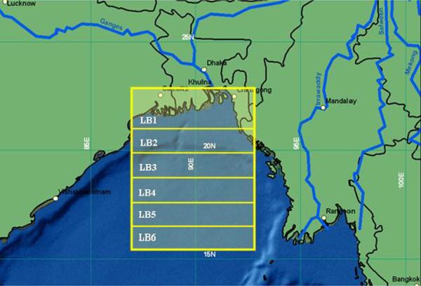
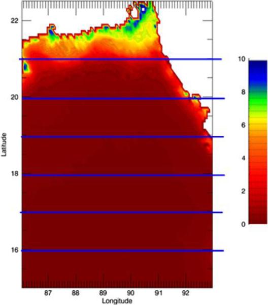
Location of Bay of Bengal study region (Yellow demarcation); LB1 to LB6 are the six latitudinal bands used in this study. (LB1: 21°N, 89.5°E; LB2: 20.25°N, 89.0°E; LB3: 19.25°N, 90.10°E; LB4: 18.75°N, 91.25°E; LB5: 17.45°N, 91.25°E; LB6: 16.25°N, 89.0°E); (b) Annual Climatology of Chlorophyll in Bay of Bengal
3. Remote Sensing of Plankton using Chlorophyll
Remote sensing of ocean started with the launch of the Coastal Zone Color Scanner on Nimbus7 in 1978, which was followed by the SeaWiFS mission in 1997. Chlorophyll measured by SeaWiFS has been used in several studies ranging from detection of harmful algal blooms (Strumf et al., 2003; Tang et al., 2003), coastal pollution (Chen et al., 2007), oceanic processes (Tang et al., 2003; Yoder et al., 1987; Danling et al., 2002, Yuras et al 2005), to land-ocean interaction (Lopez and Hidalgo, 2009; D'Sa and Miller, 2003; Jutla et al., 2009a) and marine fauna (Solanki et al., 2001; Polovina et al., 2003; Turley et al., 2000; Labiosa and Arrigo, 2003). The SeaWiFS consists of eight channels at: 412, 443, 490, 510, 555, 670, 765, and 865 nm (nanometers: 1μm = 1,000 nm), each with bandwidths of 20 or 40 nm (O'Reilly et al., 2000). The orbital altitude of SeaWiFS is about 705 km (438 mi) with spatial resolution in the Local Area Coverage of about 1.1 km (0.68 mi). The optimal resolution is 0.6 km at the nadir. Currently, SeaWiFS data offer the longest available ocean color records for more than 10 years (1997 to till date) at various spatial (4km, 9km) and temporal scales (daily, monthly, annual). Current global SeaWiFS chlorophyll algorithm, OC4V4, is a fourth-order polynomial (equation1) of the maximum band ratio of four bands (O'Reilly et al., 2000), and can be represented as:
| [1] |
where, Chl is the chlorophyll in mg/m3 and Rrs() is the wavelength in nm.
Satellite remote sensing is perhaps the best way to study and quantify large scale monitoring and variability of phytoplankton in absence of in-situ plankton data, which is prohibitively expensive to obtain. A recent study by Gregg and Casey (2004) observed a correlation of 0.78 between in-situ chlorophyll and SeaWiFS derived chlorophyll using over 2400 coastal region stations. Our study region experiences discharge from the large the Ganges, the Brahmaputra and the Meghna (GBM), river system, which bring huge amounts of freshwater containing terrestrial nutrients to the coastal waters during the summer monsoon months. There is no in-situ plankton data in the GBM coastal region; consequently we have used a proxy region for comparing applicability of SeaWiFS algorithm for the Bay of Bengal. Using subset of the chlorophyll data from SeaWiFS, Gregg and Casey (2004) reported a correlation of 0.61 between observed and measured chlorophyll close to mouth where Amazon River discharges into Atlantic Ocean. Amazon is one of the largest rivers discharging freshwater into ocean, a feature similar to the GBM river systems.
Remote sensing measurements of other relevant variables (e.g., sea surface temperature; sea surface height) may also help in understanding the possible controls on chlorophyll production in the coastal regions and its links to terrestrial hydrology. For example, using satellite measured chlorophyll from various ocean basins across the globe several recent studies suggest an inverse relationship between chlorophyll (and hence phytoplankton) and SST (e.g., Solanki et al., 2001, Uz and Yoder, 2004, Legaard and Thomas, 2006, Smyth et al. 2001). In Bay of Bengal, however, a positive relationship between phytoplankton and SST is observed (Lobitz et al., 2000; Chaturvedi, 2005; Emch et al, 2008; Magny et al., 2008). Our preliminary analyses, using SeaWiFS data, suggest that terrestrial nutrient transport through fresh water discharge from the Ganges and the Brahmaputra rivers may affect phytoplankton production in the coastal Bay of Bengal region (Jutla et al. 2011), which may also alter the usually observed inverse relationship between SST and chlorophyll. Increase in phytoplankton through freshwater discharge has been observed in several basins such as Chesapeake Bay (Acker et al., 2005), and the Delaware (Pennock and Sharp, 1985), Po (Revenlante and Gilmartim, 1976], Orinoco (Bidigare et al., 1993) and Mississippi rivers (Lohrenz et al., 1990). To summarize, space time characterization and relationship between SST and chlorophyll in Bay of Bengal is not well understood and is beyond the scope of the present study.
There are very few remote sensing related studies available for the Bay of Bengal region. Islam et al (2002) studied distribution of suspended sediments in the coastal regions of GBM region using Landsat data. According to Islam et al (2002), suspended solids play role in the estuarine regions, which are very close to the mouth of the GBM rivers draining to the Indian ocean. According to their analysis, suspended solids increase during the high flow seasons after monsoonal river discharge. However, the extent of the suspended solids in the region is limited to the estuarine region (refer to figure 1a and figure 6 of Islam et al 2002) does not appear to impact the zones specified for chlorophyll measurements in this study. Mishra et al (2008) reported a sudden increase in chlorophyll at the river mouths of the Ganges and the Brahmaputra and attributed such increase to an increased terrestrial organic load carried by volume of discharge during the monsoon season. More recently, Prasad and Singh (2010) showed a peak in chlorophyll in coastal region of Bay of Bengal after 1–2 months of peak river discharge. Our preliminary results suggest a strong relationship between terrestrial discharge and phytoplankton variability for the Bay of Bengal and three other high discharge regions of the world (Jutla et al., 2009a). Taken together, findings from these studies suggest that it is reasonable to expect that the SeaWiFS algorithms capture the spatio-temporal variability of chlorophyll in the region despite suspended solid loads during monsoonal discharge.
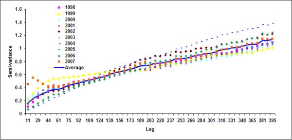
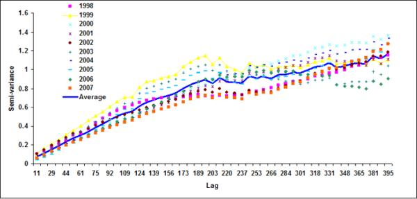
Figure 6.
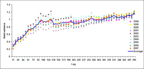
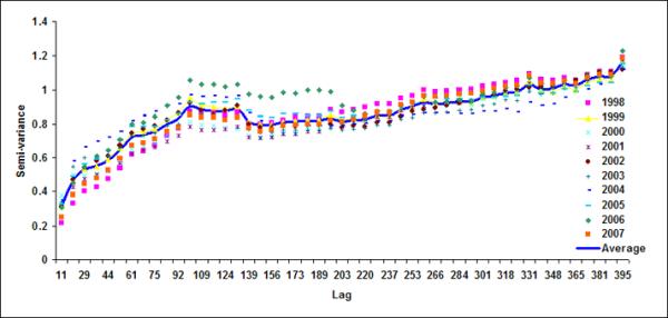


Semivariograms for LB1+LB2 for (a) October, (b) November, (c) December, (d) January (e) February and (f) March
Our analysis suggests that the average cloud cover is high (70%) during the months of May through July, while it is much lower (25%) from August through April in each of the latitudinal bands in the Bay of Bengal region. The focus of our current manuscript is to understand the implications of chlorophyll variability on two seasonal cholera outbreaks: one in the spring (defined as the average of March-April-May months) and the other in autumn (defined as the average of September-October-November months) season in Bengal Delta. Our recent study (Akanda et al., 2009, 2011) suggested that low river discharge conditions during the dry season and associated coastal intrusion of plankton water are responsible for spring cholera outbreaks in Bangladesh. Jutla et al (2010) also reported a strong correlation (r=0.81; p<0.05) between preceding autumn chlorophyll in coastal regions and spring cholera outbreaks in Bangladesh. On the other hand, autumn cholera outbreaks are strongly associated with the widespread breakdown of sanitary conditions due to flooding in the Bengal delta (Akanda et al., 2011). As streamflow direction is predominantly seaward during the high discharge season (average discharge during July-August-September months), it is highly unlikely that coastal chlorophyll is associated with autumn season cholera outbreaks since water intrusion cannot occur during this season. Therefore, the high cloud cover during summer months (Chaturvedi., 2005) in this region is not likely to significantly affect the analysis in our study.
4. Temporal Characterization of chlorophyll
4.1. Climatological chlorophyll distribution in the Bay of Bengal
We start our analysis with the annual climatological distribution of the chlorophyll in northern Bay of Bengal (Figure 1b). The climatology has been calculated by averaging monthly chlorophyll pixel values available for 10 years (1998–2007). Mean annual chlorophyll is 5.54, 1.34, 0.52, 0.33, 0.23 and 0.23 mg/m3 in LB1 through LB6, respectively. From Figure 1b it is evident that chlorophyll values are significantly higher along the coast of Bay of Bengal than in the offshore regions. As an example, chlorophyll decreases by 96% from LB1 to LB6. Chlorophyll is likely to be more along the coastal areas of Bay of Bengal because of two reasons: (a) it is the freshwater outlet region with high discharge from the GBM system (Jutla et al., 2011); and (b) coastal regions experience more upwelling compared to offshore regions (Yarus et al., 2005).
4.2 Chlorophyll variation at daily scale
With the availability of daily measurement of chlorophyll from remote sensing data, it is now possible to determine synoptic scale variability of chlorophyll in northern Bay of Bengal. Figure 2a and 2b show daily time series of chlorophyll for LB1 and LB6. On an average, the day to day variation between chlorophyll in LB1 and LB6 can vary up to 72%. A similar observation was made by Abreu et al. (2009) where they have used in-situ data along Patos Lagoon Estuary in Brazil and reported that day to day variation in chlorophyll can be as large as 60%. Figure 3 show the autocorrelation function for daily chlorophyll time series at the pixel scale (Figure 3a) and for six latitudinal bands (Figure 3b). Autocorrelation is the measure of the linear dependence of the data or the correlation in the time series with itself at different lag periods, which is used to check periodicity as well as randomness in the data (Box and Jenkins, 1991). A sharp decay in the autocorrelation structure for pixel scale (9 km) and band scale (1 degree) suggests that, at the daily scale irrespective of spatial averaging, chlorophyll time series does not have any temporal memory and resembles more like a white noise (random signal with no defined structure) signal (Figure 3). Such large variability from pixel to band levels suggests that it is not feasible to develop a predictive understanding of cholera-chlorophyll relationships at these scales.
Figure 2.
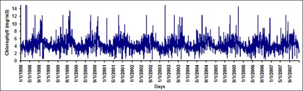

Chlorophyll time series for (a) LB1 and (b) LB6 from 1998–2007.
Figure 3.

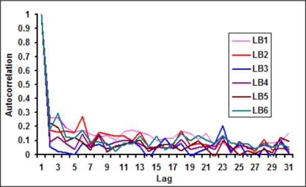
Autocorrelation function for daily chlorophyll at (a) pixel scale (LB1: 21°N, 89.5°E; LB2: 20.25°N, 89.0°E; LB3: 19.25°N, 90.10°E; LB4: 18.75°N, 91.25°E; LB5: 17.45°N, 91.25°E; LB6: 16.25°N, 89.0°E) and (b) at band scale.
4.3 Chlorophyll variation at monthly scale
As daily chlorophyll time series does not show much temporal structure, irrespective of spatial averaging from 9 km pixel scale to 1-degree band (approximately 100 km) scale, we now proceed to examine the variability of chlorophyll at a monthly time scale. Figure 4a shows monthly time series of chlorophyll in LB1. The red line is three month average chlorophyll, plotted to visualize presence of any regular variability in the time series. A seasonal maximum is usually observed in the fall season (September or October) and seasonal minima usually occur in early spring (February or March) in LB1 A closer examination of Figures 4 suggests that the underlying governing processes for LB1 and LB2 are different than those of the offshore bands. For example, chlorophyll variability for LB1 and LB2 shows distinct seasonality as evident from their autocorrelation function (Figure 5) with very high lag 1 autocorrelation suggesting strong month to month persistence.
Figure 4.
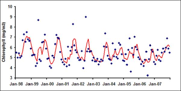
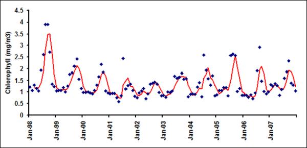
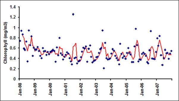


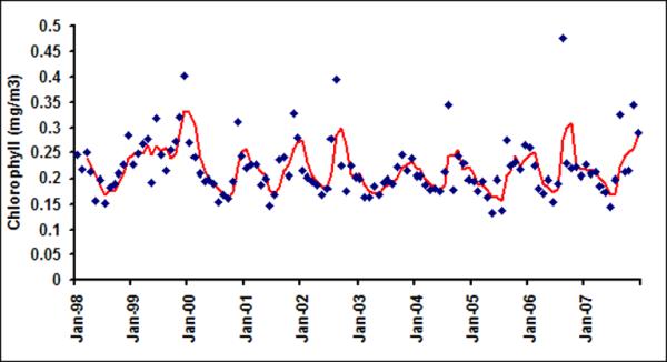
Monthly chlorophyll in six latitudinal bands (a) LB1; (b) LB2; (c) LB3; (d)LB4; (e) LB5 and (f) LB6
Figure 5.
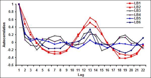
Autocorrelation function for monthly chlorophyll for six latitudinal bands
For the offshore bands (LB3 through LB6), on the other hand, there is no discernable periodicity and lag 1 autocorrelation is low. There are no statistically significant peaks (greater than 1/e: 0.37) at any lag for all the bands except for LB1 and LB2. Thus, from here on, we will focus our analysis on the coastal bands (defined as LB1 and LB2 combined) and the offshore bands (LB5 and LB6 combined) only.
For the coastal bands, monthly chlorophyll time series shows significant memory (Figure 5); yet at the pixel scale (9 km) it does not exhibit much persistence in time; for all pixels in coastal bands show very low lag one autocorrelation (0.12±0.24). With increased spatial averaging, temporal persistence of monthly chlorophyll increases and lag one autocorrelation stabilizes at around 0.60 for 1296 km2 or larger areal averages (Table 1). These results suggest that to have a reasonable prediction lead time, one needs to aggregate chlorophyll time series to monthly scales along with a spatial averaging scale of 1296 km2 or larger.
Table 1.
Lag 1 autocorrelation as a function of spatial averaging for LB1 and LB2
| Pixel size (km) | Sample (P1) Centered 21°N, 88°E | Sample (P2) Centered 21.5°N, 90°E |
|---|---|---|
| 1×1 | 0.10 | 0.55 |
| 2×2 | 0.34 | 0.56 |
| 3×3 | 0.45 | 0.60 |
| 4×4 | 0.58 | 0.64 |
| 5×5 | 0.63 | 0.61 |
| 6×6 | 0.61 | 0.63 |
5. Spatial Characterization of Chlorophyll in the Bay of Bengal
Understanding spatial variability of phytoplankton is important since such variability at different scales may indicate growth, distribution and survival of planktonic species, plan for efficient use of instrumentation but most importantly, identify possible controls on plankton production (Steele 1976; Walsh 1978; Valiela 1984; Mackas 1984; Campbell and Esaias 1985). Within this context, the goal of spatial analysis is to compare and contrast the variability of chlorophyll in the coastal and offshore regions. Geostatistical technique, such as the semivariogram analysis, is often used to characterize and understand spatial patterns geophysical variables, such as soil moisture (Entin et al., 2000; Mohanty et al., 2000; Western et al., 2002), precipitation (Hevesi et al., 1992; Bachhi & Kottegoda, 1995). A key concept in geostatistics, the variogram, describes the variance between the points in a spatial field as a function of their separation distances (Western et al., 2004). Three main structural parameters of the variogram are the sill, the range or the correlation length, and the nugget. The sill is the point where the semi-variogram flattens out. The range or the correlation length determines the spatial continuity of the variable of interest. The range is the distance beyond which the correlation between points is minimal. If there exists a sill in the semivariogram, the spatial distribution of the variable is stationary upto the range or correlation length. The nugget determines the variance between pairs of points separated by very small distances, which are a combination of measurement error and small-scale variability that cannot be distinguished from the spatial dataset (Western et al., 2004).
5.1 Spatial Structure of Chlorophyll at Monthly Scale
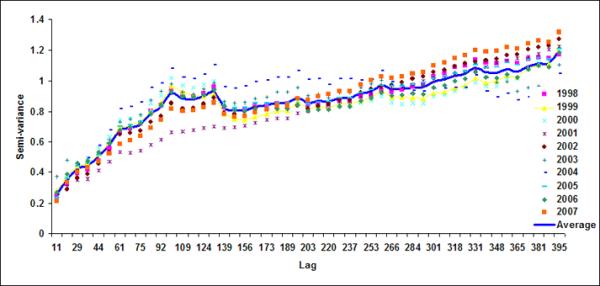
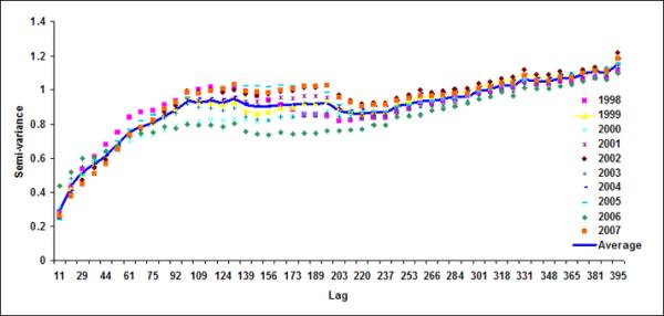
Spatial geostatistical analysis was conducted on ten years of chlorophyll data using geostatistical software GSLIB (Deutsch & Journel, 1992). Figure 6 shows monthly semivariograms for six months (October to March) for the coastal band. The choice of these six months is motivated by the dynamics of cholera outbreaks in the Bengal delta as well as accuracy of satellite data. As mentioned before, the autumn (~October) peak of cholera outbreaks has been associated with the hydrology of the region (such as floods), the spring (~March) peak is associated with the coastal processes in Bay of Bengal, such as intrusion of coastal waters into inland water bodies (Akanda et al., 2009). These six months (October through March) are also relatively cloud free for the Bay of Bengal region (Chaturvedi, 2005) and hence provide better accuracy for chlorophyll measurements from satellites. Figure 6 shows the semivariogram for coastal bands; the solid line shows the average semivariogram for ten years of data. To define the sill in the semi-variogram, we followed a procedure similar to Yoder et al (1987): a decrease in the slope to 10% or less of the mean slope before it decreases; constant (±10%) or decreasing semivariance after the break in the slope; and sill value is at least twice as that of the nugget variance. Based on this criterion, for the coastal band, we observe a range or a correlation length of 102, 92, 104, 105, 108, 106 km for October, November, December, January, February and March months respectively. Average observed correlation length for these six months in the coastal band is about 100km. The offshore band (Figure 7), on the other hand, does not have a defined correlation length except for the month of January (correlation length ~200km). This, presence (absence) of correlation length in the coastal (offshore) bands, indicates that the two regions have two separate processes controlling the production and space-time variability of phytoplankton. Such a regional demarcation of chlorophyll in Bay of Bengal has significant implications for understanding and modeling cholera-plankton relationships.
Figure 7.
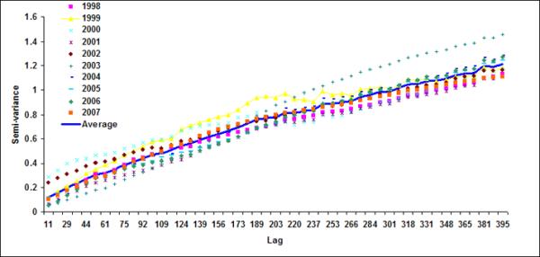
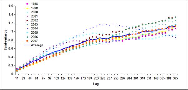

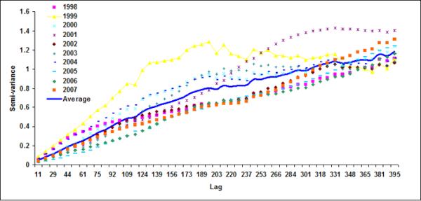
Semivariograms for LB5+LB6 for (a) October, (b) November, (c) December), (d) January, (e) February and (f) March
Using variogram analysis along the continental southeastern United States, Yoder et al (1987) indicated that the correlation length in the coastal regions is smaller than the offshore waters. Two major reasons for shorter correlation lengths in coastal regions than those for the offshore regions were given as: (a) mesoscale ocean current variability caused by eddies (Gower et al., 1980; Karhu et al., 1982; Yoder et al., 1987) and (or) (b) addition of terrestrial nutrient and consequent increase in phytoplankton (Mackas, 1984; Campbell & Esaias, 1985). In coastal region of Bay of Bengal, freshwater discharge from the two major rivers, the Ganges and the Brahmaputra, substantially increase terrestrial nutrient fluxes (Sheyte, 1996) and thereby may affect the correlation length for the coastal band. Absence of a defined correlation length in the offshore region indicates that chlorophyll variability is perhaps controlled by large-scale oceanic processes, such as frontal eddies (Yoder et al., 1987; McClain et al., 1984).
6. Cholera and Space-Time variability of Chlorophyll
The findings from sections 4 and section 5 have direct implications on understanding plankton-cholera relationships in the Northern Bay of Bengal. We have established that chlorophyll in the coastal band (LB1+LB2) shows a distinct annual cycle. Cholera incidence data were acquired from a surveillance system maintained by the International Centre for Diarrheal Disease Research, Bangladesh (ICDDR,B), where incidence is recorded as the percent of new cholera infected patients among a statistical subset of patients selected from a total pool of patients visiting the hospital for treatment during a given week (Longini, 2002). Figure 8 shows climatological monthly cholera and coastal chlorophyll for ten years (1998–2007). Cholera incidence in the Bay of Bengal region exhibit bi-annual peaks; one in autumn season and the other in spring seasons (Figure 8). However, coastal chlorophyll shows only one seasonal peak in autumn season. The presence of a single peak in chlorophyll and double peak in cholera suggests that chlorophyll variability may not be the only variable affecting cholera outbreaks.
Figure 8.

Annual Cholera and Coastal Chlorophyll in Bay of Bengal. Monthly cholera time series were obtained from International Center for Diarrhoeal Disease Research in Bangladesh (ICDDR,B).
Based on our current understanding (Akanda et al., 2009) high river discharge from the GBM rivers are responsible for the autumn peak in cholera outbreaks, whereas the spring peak is related to low flow discharges and subsequent intrusion of coastal plankton laden seawater. The high levels of chlorophyll during autumn is unlikely to be responsible for the simultaneous outbreaks in autumn since the river discharge is high in this season; making it impossible for plankton to get into inland water systems. On the other hand, plankton abundance in autumn may lead to cholera in the spring season through various mechanisms, such as the one suggested by Seeligmann et al. (2008) and Binsztein et al. (2004). Historically, it is observed that cholera bacteria activity subsides with the onset of winter (Cliff et al., 2004). Binsztein et al. (2004) suggested that cholera bacteria may enter the dormant non-culturable state with the onset of winter, and under favorable condition(s), the bacteria can become viable and cause epidemic. During low discharge months, intrusion of chlorophyll through river networks, under favorable conditions, may lead to cholera outbreaks in spring seasons. Also, Huq and Colwell (1983, 1995) suggested that cholera bacteria require zooplankton for survival that in turn feed on the phytoplankton in the coastal waters, therefore the presence of lagged relationship between spring cholera outbreaks and autumn chlorophyll may be justified. Sack et al. (2003) have indicated that the spring outbreaks of cholera are primarily observed in the coastal region of Bay of Bengal. Correlation between autumn chlorophyll and spring cholera is about 0.81, suggesting that spring cholera outbreaks may be related to previous autumn chlorophyll (Jutla et al., 2009b). Such high correlation between chlorophyll and cholera makes coastal chlorophyll a likely variable to be used in development of any predictive models for spring cholera outbreaks.
Concurrent correlation between monthly cholera and coastal band chlorophyll time series (Figure 9a) is about 0.45. For the offshore region, this correlation between cholera and chlorophyll (Figure 9b) drops to about 0.10. This is another indication that chlorophyll measurements in the coastal band are likely to play an important role in understanding plankton-cholera relationships. Plausible lead-lag relationships between chlorophyll and cholera need to be explored in future studies.
Figure 9.
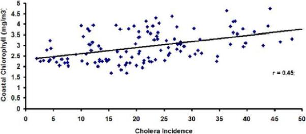
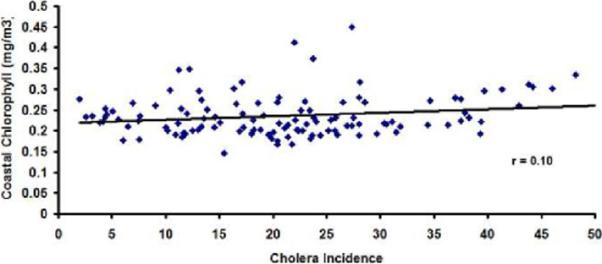
Correlation plot between monthly cholera incidence and (a) Coastal, (b) Offshore chlorophyll in the Bay of Bengal region.
7. Discussion
Endimicity of cholera in the Bengal Delta and a strong laboratory based relationship between cholera and plankton abundance motivated this study to explore the spatial and temporal variability of chlorophyll in northern Bay of Bengal. Space-time characterization of chlorophyll is an essential first step to establish relationship between cholera and plankton abundance over a range of scales. Using ten years of daily SeaWiFS chlorophyll data, we have established that chlorophyll time series is a white noise (defined as random process with no defined structure) process for pixel (~10km) to band (~100 km) scales. We also note that the large temporal variations of pixel level chlorophyll concentration put a practical constraint on the design and implementation of in-situ plankton measurements for coastal areas. Such large temporal variations of pixel level chlorophyll concentration put a practical constraint on the design and implementation of in-situ plankton measurements for coastal areas. These results are similar to those of Uz & Yoder (2004) who also suggested that variability of chlorophyll, along Southeastern US Continental shelf, on daily time scale resembles a white noise process with significant day to day variability in coastal as well as in open ocean waters
Results of chlorophyll variability at the monthly time scale are more encouraging. We have established that chlorophyll in the coastal band shows a distinct annual cycle while such a cycle is not apparent for offshore regions. For the coastal bands, monthly chlorophyll time series shows significant memory; yet at the pixel scale (9 km) it does not exhibit much persistence in time. With increased spatial averaging, temporal persistence of monthly chlorophyll increases. An aggregated monthly chlorophyll concentration for the coastal band - with a spatial averaging scale of 1296 km2 or larger - is likely to provide a lower limit on spatial scale of plankton measurements for a useful prediction lead time for a potential cholera outbreak model.
Peak chlorophyll levels in the coastal band tend to occur in the autumn season, whereas lowest chlorophyll is observed in early spring season. On the other hand, chlorophyll in offshore regions of Bay of Bengal does not exhibit any preferential seasonal maxima or minima. A plausible reason for the presence of an annual cycle in chlorophyll variability for the coastal band may be attributed to large freshwater discharge and associated terrestrial nutrient influx from two rivers, the Ganges and the Brahmputra, into the northern Bay of Bengal. A peak discharge for these two rivers is observed in August (Dai & Trenberth, 2001) while peak chlorophyll is observed in September. River discharges have been associated with the increase of phytoplankton from other coastal regions as well (Arker et al., 2005; Smith & Demaster, 1996; Lopez & Hidalgo, 2009). Spatial analysis indicates that chlorophyll in the coastal band has a correlation length of approximately 100km whereas offshore bands have no well-defined correlation length. The dominance of different space-time variations for coastal and offshore chlorophyll suggests that physical processes and drivers for chlorophyll are indeed different in the two regions. These results suggest that physical processes and drivers for chlorophyll may be different in the coastal and offshore regions.
To our best knowledge, this is perhaps one of the first studies to examine cholera-chlorophyll relationship over such a large range of spatial and temporal scales in northern Bay of Bengal using satellite data. We recognize that the SeaWiFS chlorophyll data is likely to be noisy due to sediments, organic and inorganic matter particularly close to the coastal areas (Martin, 2004). However, NASA's latest OC4v4 chlorophyll algorithm has correction already applied to the data. In the presence of sediments, the correction algorithm shifts to a higher wavelength to maintain high signal to noise ratio (Martin, 2004). Several recent studies (e.g., Legaard & Thomas (2006), Uz & Yoder (2004), Doney et al., (2003), Chaturvedi (2005)) demonstrate that the SeaWiFS sensor has been reasonably stable over the years of operation and calibration approach provided consistent global water-leaving radiances, and the products meet the accuracy goals over a diverse set of open ocean validation sites (McClain et al 1998; Gregg and Casey, 2004). A key strength of the SeaWiFS dataset is that, despite the inherent measurement accuracy and noise level, it captures the seasonal dynamics of chlorophyll in coastal regions. Although pixel level chlorophyll values have uncertainty and noise, it is the “contextual information” of neighboring pixels that make this data set a useful tool for our analysis.
An important implication of this study is likely to be on the design of in-situ sampling strategies of coastal chlorophyll in northern Bay of Bengal to establish plankton-cholera relationships. Given the day to day variability of chlorophyll for a range of spatial scales, findings from this study suggest that continuous measurements of plankton will be necessary for an extended period of time to develop any meaningful time series for analysis and model development. Although chlorophyll measurement from satellites eliminates detailed field sampling needs over large regions; yet, to establish limits of accuracy of satellite measurements as well as to relate chlorophyll measurements with phytoplankton types, in-situ measurements will be needed. Findings from this study further suggest that daily chlorophyll concentration may not be particularly useful to develop any cholera predictive model. We do recognize that comprehensive monthly and seasonal scale analyses are needed, in future, to explore synchronous as well as lead-lag relationships between coastal chlorophyll variability and cholera outbreaks in inland locations during subsequent seasons.
Research Highlights
Variability of chlorophyll at daily scale resembles white noise.
At a monthly scale, chlorophyll shows distinct seasonality.
Spatial analyses indicate presence of two separate processes for production of chlorophyll in coastal and offshore regions.
Puts a lower limit on space-time averaging of plankton at 1296 km2-monthly scale to establish relationships with cholera incidence.
Footnotes
Publisher's Disclaimer: This is a PDF file of an unedited manuscript that has been accepted for publication. As a service to our customers we are providing this early version of the manuscript. The manuscript will undergo copyediting, typesetting, and review of the resulting proof before it is published in its final citable form. Please note that during the production process errors may be discovered which could affect the content, and all legal disclaimers that apply to the journal pertain.
References
- Abreu PC, Bergesch M, Proença LA, Garcia CAE, Odebrecht C. Short- and long-term chlorophyll a variability in the shallow microtidal Patos Lagoon Estuary, Southern Brazil. Estuaries and Coasts. 2009 DOI 10.1007/s12237-009-9181-9. [Google Scholar]
- Acker JG, Harding LW, Leptoukh G, Zhu T, Shen S. Remotely-sensed chl-a at the Chesapeake Bay mouth is correlated with annual freshwater flow to Chesapeake Bay. Geophysical Research Letters. 2005;32:L05601. doi:10.1029/2004GL021852. [Google Scholar]
- Akanda SA, Jutla AS, Islam S. Dual Peak Cholera Transmission in Bengal Delta: A Hydroclimatological Explanation. Geophysical Research Letters. 2009 DOI: doi:10.1029/2009GL039312. [Google Scholar]
- Akanda AS, Jutla AS, Constantin de Magny G, Alam M, Siddique AK, Sack RB, Huq A, Colwell RR, Islam S. Hydroclimatic Influences on Seasonal and Spatial Cholera Transmission Cycles: Implications for Public Health Intervention in the Bengal Delta. Water Resources Research. 2010;47:W00H07. doi:10.1029/2010WR009914. [Google Scholar]
- Alam M, Sultana M, Nair GB, Sack RB, Sack DA, Siddique AK, Ali A, Huq A, Colwell RR. Toxigenic Vibrio cholerae in the Aquatic Environment of Mathbaria, Bangladesh. Applied Environmental Microbiology. 2006;72:2849–2855. doi: 10.1128/AEM.72.4.2849-2855.2006. [DOI] [PMC free article] [PubMed] [Google Scholar]
- Alam M, Sultana M, Balakrish Nair G, Siddique AK, Hasan NA, Bradley Sack R, et al. Viable but nonculturable vibrio cholerae O1 in biofilms in the aquatic environment and their role in cholera transmission. Proceedings of the National Academy of Sciences of the United States of America. 2007;104(45):17801–17806. doi: 10.1073/pnas.0705599104. [DOI] [PMC free article] [PubMed] [Google Scholar]
- Bacchi B, Kottegoda NT. Identification and calibration of spatial correlation patterns of rainfall. Journal of Hydrology. 1995;165:311–348. [Google Scholar]
- Bidigare RR, Ondrusek M, Brooks J. Influence of the Orinoco river outflow on distributions of algal pigments in the Caribbean Sea. J. Geophy. Res. 1993;98:2259–2269. [Google Scholar]
- Binsztein N, Costagliola MC, Pichel M, Jurquiza V, Ramirez FC, Akselman R, Vacchino M, Huq A, Colwell R. Viable but Nonculturable Vibrio cholerae O1 in the Aquatic Environment of Argentina. Applied Environmental Microbiology. 2004;70:7481–7486. doi: 10.1128/AEM.70.12.7481-7486.2004. [DOI] [PMC free article] [PubMed] [Google Scholar]
- Box G, Jenkins MG. Time Series Analysis: Forecasting & Control. 2rd Edition Prentice-Hall; USA: 1991. [Google Scholar]
- Campbell JW, Esaias WE. Spatial patterns in temperature and chlorophyll on Nantucket Shoals from airborne remote sensing data, May 7–9, 1981. Journal of Marine Research. 1985;43:139–161. [Google Scholar]
- Chaturvedi N. Variability of chlorophyll concentration in the Arabian Sea and Bay of Bengal as observed from SeaWiFS data from 1997–2000 and its interrelationship with Sea Surface Temperature (SST) derived from NOAA AVHRR. International Journal of Remote Sensing. 2005;26:3695–3706. [Google Scholar]
- Chen C, Tang S, Pan Z, Zhan H, Larson M, Jönsson L. Remotely Sensed Assessment of Water Quality Levels in the Pearl River Estuary, China. Mar. Poll. Bull. 2007;54(8):1267–1272. doi: 10.1016/j.marpolbul.2007.03.010. [DOI] [PubMed] [Google Scholar]
- Colwell RR, Huq A, Islam MS, Aziz KMA, Yunus M, Huda Khan N, et al. Reduction of cholera in Bangladeshi villages by simple filtration. Proceedings of the National Academy of Sciences of the United States of America. 2003;100(3):1051–1055. doi: 10.1073/pnas.0237386100. [DOI] [PMC free article] [PubMed] [Google Scholar]
- Cliff A, Haggett P, Smallman-Raynor M. World Atlas of Epidemic Diseases. Arnold Publication; UK: 2004. [Google Scholar]
- Dai A, Trenberth KE. Estimates of Freshwater Discharge from Continents: Latitudinal and Seasonal Variations. Journal of Hydrometeorology. 2002;3:660–687. [Google Scholar]
- Danling T, Kester DR, Ni I, Kawamura H, Huasheng H. Upwelling in the Taiwan Strait during the Summer Monsoon Detected by Satellite and Shipboard Measurements. Remote Sens.Environ. 2002;83(3):457–471. [Google Scholar]
- Deutsch CV, Journel AG. GSLIB: Geostatistical Software Library and User's Guide. Oxford University Press; Oxford: 1992. [Google Scholar]
- Doney SC, Glover DM, McCue SJ, Fuentes M. Mesoscale variability of SeaWiFS satellite ocean color: global patterns and spatial scales. Journal of Geophysical Research. 2003;108(C2) doi:10.1029/2001JC000843. [Google Scholar]
- D'Sa EJ, Miller RL. Bio-optical Properties in Waters Influenced by the Mississippi River During Low Flow Conditions. Remote Sens. Environ. 2003;84(4):538–549. [Google Scholar]
- Emch M, Feldacker C, Yunus M, Streatfield PK, Thiem V, Cahn D, Mohammad A. Local Environmental Predictors of Cholera in Bangladesh and Vietnam. American Journal of Tropical Medicine and Hygiene. 2008;78:823–832. [PubMed] [Google Scholar]
- Entin JK, Robock A, Vinnikov KY, Hollinger SE, Liu S, Namkhai A. Temporal and spatial scales of observed soil moisture variations in the extratropics. Journal of Geophysical Research. 2000;105(D9):11,865–11,877. [Google Scholar]
- Epstein PR. Algal Blooms in the Spread and Persistence of Cholera. Biosystems. 1993;31:209–221. doi: 10.1016/0303-2647(93)90050-m. [DOI] [PubMed] [Google Scholar]
- Gower JF, Denman KL, Holyer RJ. Phytoplankton patchiness indicates the fluctuation spectrum of mesoscale oceanic structure. Nature. 1980;288:157–159. [Google Scholar]
- Gregg WW, Casey NW. Global and regional evaluation of the SeaWiFS chlorophyll data set. Remote Sensing of Environment. 2004;93:463–479. [Google Scholar]
- Hevesi JA, Istok JD, Flint AL. Precipitation estimation in mountainous terrain using multivariate geostatistics. Part I: structural analysis. Journal of Applied Meteorology. 1992;317:661–676. [Google Scholar]
- Huq A, Colwell RR. Vibrios in the Marine and Estuarine Environment: Tracking Vibrio cholerae. Ecosystem Health. 1996;2(3):198–214. [Google Scholar]
- Huq A, West PA, Small EB, Huq MI, Colwell RR. Influence of water temperature, salinity, and ph on survival and growth of toxigenic Vibrio-Cholerae sero-O1 associated with live copepods in laboratory microcosms. Applied Environmental Microbioliology. 1984;48(2):420–424. doi: 10.1128/aem.48.2.420-424.1984. [DOI] [PMC free article] [PubMed] [Google Scholar]
- Huq A, Sack RB, Nizam A, Longini IM, Nair GB, Ali A, et al. Critical factors influencing the occurrence of vibrio cholerae in the environment of Bangladesh. Applied and Environmental Microbiology. 2005;71(8):4645–4654. doi: 10.1128/AEM.71.8.4645-4654.2005. [DOI] [PMC free article] [PubMed] [Google Scholar]
- Islam MR, Begum SF, Yamaguchi Y, Ogawa K. Distribution of suspended sediments in the coastal sea off the Ganges-Brahmputra River mouth: observation from TM data. Journal of Marine Systems. 2002;32:307–321. [Google Scholar]
- Jutla AS, Akanda AS, Islam S. Tracking Cholera in Coastal Regions using Satellite Observations. Journal of American Water Resources Association. 2010:1–12. doi: 10.1111/j.1752-1688.2010.00448.x. DOI:10.1111/j.1752-1688.2010.00448.x. [DOI] [PMC free article] [PubMed] [Google Scholar]
- Jutla AS, Akanda AS, Griffiths J, Islam S, Colwell R. Warming oceans, phytoplankton, and river discharge: Implications for cholera outbreaks. American Journal of Tropical Medicine and Hygiene. 2011 doi: 10.4269/ajtmh.2011.11-0181. doi:10.4269/ajtmh.2011.11-0181. [DOI] [PMC free article] [PubMed] [Google Scholar]
- Jutla AS, Small D, Islam S. A precipitation dipole in Eastern North America. Geophysical Research Letters. 2006;33:L21703. doi:10.1029/2006GL027500. [Google Scholar]
- Jutla AS, Akanda S, Islam S. Satellites and Human Health: Potential for Tracking Cholera Outbreaks. Proceedings of the American Geophysical Union; San Francisco, California. Dec 14–18, 2009. [Google Scholar]
- Karhu MK, Autsam A, Elken J. Spatio-temporal dynamics of chlorophyll in the open Baltic Sea. Journal of Plankton Research. 1982;4:779–790. [Google Scholar]
- Labiosa RG, Arrigo KR. The interplay between Upwelling and Deep Convective Mixing in Determining the Seasonal Phytoplankton Dynamics in the Gulf of Aqaba: Evidence from SeaWiFS and MODIS. Limnol. Oceanogr. 2003;48(6):2355–2368. [Google Scholar]
- Legaard KL, Thomas AC. Spatial patterns in seasonal and interannual variability of chlorophyll and sea surface temperature in the California current. Journal of Geophysical Research. 2006;111:C06032. doi:10.1029/2005JC003282. [Google Scholar]
- Lobitz BM, Beck LR, Huq A, Wood B, Fuchs G, Faruque ASG, Colwell RR. Climate and infectious disease: use of remote sensing for detection of Vibrio Cholerae by indirect measurement. PNAS. 2000;97(4):1438–1443. doi: 10.1073/pnas.97.4.1438. [DOI] [PMC free article] [PubMed] [Google Scholar]
- Lohrenz SE, Dagg MJ, Whitledge TE. Enhanced primary production at the plume/oceanic interface of the Mississippi River. Continental Shelf Res. 1990;10:639–664. [Google Scholar]
- Longini IM, Yunus M, Zaman K, Siddique AK, Sack BB. Epidemic and endemic cholera trends over a 33-year period in Bangladesh. Journal of Infectious Diseases. 2002;186:246–251. doi: 10.1086/341206. [DOI] [PubMed] [Google Scholar]
- Lopez BM, Hidalgo JZ. Seasonal and interannual variability of cross-shelf transports of chlorophyll in the Gulf of Mexico. Journal of Marine Sciences. 2009;77(1–2):1–20. [Google Scholar]
- Mackas DL. Spatial autocorrelation of plankton community composition in a continental shelf ecosystem. Limnological Oceanography. 1984;29:451–471. [Google Scholar]
- Magny G, Murtugudde R, Sapianob M, Nizam A, Brown C, Busalacchi A, Yunus M, Nair G, Gil A, Calkins J, Manna B, Rajendran K, Bhattacharya M, Huq A, Sack R, Colwell R. Environmental signatures associated with cholera epidemics. PNAS. 2008;105(46) doi: 10.1073/pnas.0809654105. doi:10.1073/pnas.0809654105. [DOI] [PMC free article] [PubMed] [Google Scholar]
- Martin S. An Introduction to Ocean Remote Sensing. Cambridge University Press; USA: 2004. [Google Scholar]
- Matheron G. Principles of Geostatistics. Economic Geology. 1963;58:1246–1266. [Google Scholar]
- McClain CR, Cleave ML, Feldman GC, Gregg WW, Hooker SB, Kuring N. Science quality SeaWiFS data for global biosphere research. Sea Technology. 1998;39:10–16. [Google Scholar]
- McClain CR, Pietrafesa LJ, Yoder JA. Observations of Gulf stream induced and wind driven upwelling in the Georgia Bight using ocean color and infrared imagery. Journal of Geophysical Research. 1984;89:3705–3723. [Google Scholar]
- Mishra RK, Shaw BP, Sahu BK, Mishra S, Senga Y. Seasonal appearance of Chlorophyceae phytoplankton bloom by river discharge off Paradeep at Orissa Coast in the Bay of Bengal. Environ. Monit. Assess. 2008 doi: 10.1007/s10661-008-0200-2. 2008. 10.1007/s10661-008-0200-2. [DOI] [PubMed] [Google Scholar]
- Mohanty BP, Famiglietti JS, Skaggs TH. Evolution of soil moisture spatial structure in a mixed vegetation pixel during the Southern Great Plains 1997 (SGP97) hydrology experiment. Water Resources Research. 2000;36(12):3675–3686. [Google Scholar]
- Nezlin NP, Li LB. Time-series analysis of remote-sensed chlorophyll and environmental factors in the Santa Monica-San Pedro Basin off Southern California. Journal of Marine Systems. 2003;39(3–4):185–202. [Google Scholar]
- Olsson T. Malaria and cholera are traced by satellites. Lakartidningen. 1996;93(36):3037–40. [PubMed] [Google Scholar]
- O'Reilly JE, Maritorena S, Siegel D, O'Brien MC, Toole D, Mitchell BG, et al. Ocean color chlorophyll a algorithms for SeaWiFS, OC2, and OC4. In: Hooker SB, Firestone ER, editors. SeaWiFS postlaunch technical report series, SeaWiFS postlaunch calibration and validation analyses, Part 3. Version 4 vol. 11. NASA/GSFC; 2000. pp. 9–23. [Google Scholar]
- Pennock JR, Sharp JH. Phytoplankton production in the Delaware Estuary: temporal and spatial variability. Estuarine,Coastal and Shelf Science. 1985;21:711–725. [Google Scholar]
- Polovina JJ, Balaz GH, Howell EA, Parker DM, Seki MP, Dutton PH. Forage and Migration Habitat of Loggerhead (Caretta caretta) and Olive Ridley (Lepidochelys olivacea) Sea Turtles in the Central North Pacific Ocean. Fisheries Oceanogr. 2003;13(1):36–51. [Google Scholar]
- Prasad AK, Singh RP. Chlorophyll, calcite, and suspended concentrations in the Bay of Bengal and the Arabian Sea at the river mouths. Advances in Space Research. 2010;45:61–69. [Google Scholar]
- Reidl J, Klose KE. Vibrio Cholerae and cholera: out of the water and into the host. FEMS Microbiology Reviews. 2002;26(2):125–139. doi: 10.1111/j.1574-6976.2002.tb00605.x. [DOI] [PubMed] [Google Scholar]
- Revelante N, Gilmartin M. The effect of Po River discharge on phytoplankton dynamics in the Northern Adriatic Sea. Marine Biology. 1976;34:259–271. [Google Scholar]
- Sack RB, Siddique AK, Huq A, Longini IM, Nair GB, Qadri F, Yunus M, Albert MJ, Sack DA, Colwell RR. A 4-Year study of the epidemiology of Vibrio Cholerae in four rural areas of Bangladesh. Journal of Infectious Diseases. 2003;187:96–101. doi: 10.1086/345865. [DOI] [PubMed] [Google Scholar]
- Seeligmann CT, Mirande V, Tracanna BC, Silva C, Aulet O, Cecilia M, Binsztein N. Phytoplankton-linked viable non-culturable Vibrio cholerae O1 (VNC) from rivers in Tucuman, Argentina. Journal of Plankton Research. 2008;30:367–377. [Google Scholar]
- Shetye SR. The movement and implications of the Ganges–Brahmaputra runoff on entering the Bay of Bengal. Current Science. 1996;64(1):32–38. [Google Scholar]
- Smith WO, Demaster DJ. Phytoplankton biomass and productivity in the Amazon River plume: correlation with seasonal river discharge. Continental Shelf Research. 1996;16(3):291–319. [Google Scholar]
- Smyth TJ, Miller PI, Groom SB, Lavender SJ. Remote Sensing of Sea Surface Temperature and Chlorophyll during Lagrangian Experiments at the Iberian Margin. Prog. Oceanogr. 2001;51:269–281. [Google Scholar]
- Solanki HU, Dwivedi RM, Nayark SR. Synergistic Analysis of SeaWiFS Chlorophyll Concentration and NOAA-AVHRR SST Feature for Exploring Marine Living Resources. Int. J. Rem. Sens. 2001;22:3877–3882. [Google Scholar]
- Stumpf RP, Culver ME, Tester PA, Tomlinson M, Kirkpatrick GJ, Pederson BA, Truby E, Ransibrahmanakul V, Soracco M. Monitoring Karenia Brevis Blooms in the Gulf of Mexico using Satellite Ocean Color Imagery and Other Data. Harmful Algae. 2003;2(2):147–160. [Google Scholar]
- Tamplin ML, Gauzens AL, Huq A, Sack DA, Colwell RR. Attachment of Vibrio cholerae serogroup O1 to zooplankton and phytoplankton of Bangladesh waters. Applied Environmental Microbioliology. 1990;56(6):1977–1980. doi: 10.1128/aem.56.6.1977-1980.1990. [DOI] [PMC free article] [PubMed] [Google Scholar]
- Tang D, Kester DR, Ni I, Qi Y, Kawamura H. In Situ and Satellite Observations of A Harmful Algal Bloom And Water Condition at The Pearl River Estuary in Late Autumn 1998. Harmful Algae. 2003;2(2):89–99. [Google Scholar]
- Turley CM, Bianchi M, Christaki U. Relationship between Primary Producers and Bacteria in an Oligotrophic Sea - The Mediterranean And Biogeochemical Implications. Mar. Eco.-Prog. Ser. 2000;193:11–18. [Google Scholar]
- Uz BM, Yoder JA. High Frequency and Mesoscale Variability in SeaWiFS Chlorophyll Inagery and its Relation to Other Remotely Sensed Oceanographic Variables. Deep-Sea Res-II. 2004;51:1001–1071. [Google Scholar]
- Western AW, Grayson RB, Blöschl G. Scaling of soil moisture: a hydrologic perspective. Annual Review of Earth and Planetary Sciences. 2002;205:20–37. [Google Scholar]
- Western AW, Zhou S, Grayson RB, McMahon TA, Blöschl G, Wilson DJ. Spatial correlation of soil moisture in small catchments and its relationship to dominant spatial hydrological processes. Journal of Hydrology. 2004;286:113–134. [Google Scholar]
- Yoder JA, McClain CR, Blanton JO, Oey L. Spatial Scales in CZCS-chlorophyll Imagery of the Southeastern US Continental Shelf. Limnological Oceanography. 1987;32(4):924–941. [Google Scholar]
- Yuras G, Ulloa O, Hormaza'bal S. On the annual cycle of coastal and open ocean satellite chlorophyll off Chile (18-40S) Geophysical Research Letters. 2005;32:L23604. doi:10.1029/2005GL023946. [Google Scholar]
- Campbell JW, Esaias WE. Spatial patterns in temperature and chlorophyll on Nantucket Shoals from airborne remote sensing data, May 7–9, 1981. J. Mar. Res. 1985;43:139–161. [Google Scholar]
- Mackas DL. Spatial autocorrelation of plankton community composition in a continental shelf ecosystem. Limnol. Oceanogr. 1984;29:451–471. [Google Scholar]
- Steele JH. Patchiness. In: Cushing DH, Walsh JJ, editors. The ecology of the seas. Blackwell; 1976. pp. 98–115. [Google Scholar]
- Walsh JJ. The biological consequences of interaction of the climatic, el nino, and event scales of variability in the eastern tropical Pacific. Rapp. P.-V. Reun. Cons. Int. Explor. Mer. 1978;173:182–192. [Google Scholar]
- Valiela I. Marine ecological processes. Springer; 1984. [Google Scholar]