Abstract
Purpose: The authors present an efficient method for generating anthropomorphic software breast phantoms with high spatial resolution. Employing the same region growing principles as in their previous algorithm for breast anatomy simulation, the present method has been optimized for computational complexity to allow for fast generation of the large number of phantoms required in virtual clinical trials of breast imaging.
Methods: The new breast anatomy simulation method performs a direct calculation of the Cooper’s ligaments (i.e., the borders between simulated adipose compartments). The calculation corresponds to quadratic decision boundaries of a maximum a posteriori classifier. The method is multiscale due to the use of octree-based recursive partitioning of the phantom volume. The method also provides user-control of the thickness of the simulated Cooper’s ligaments and skin.
Results: Using the proposed method, the authors have generated phantoms with voxel size in the range of (25–1000 μm)3/voxel. The power regression of the simulation time as a function of the reciprocal voxel size yielded a log-log slope of 1.95 (compared to a slope of 4.53 of our previous region growing algorithm).
Conclusions: A new algorithm for computer simulation of breast anatomy has been proposed that allows for fast generation of high resolution anthropomorphic software phantoms.
Keywords: modeling, visualization, validation, simulation of clinical breast imaging
INTRODUCTION
Breast tissue simulation is of importance for developing anthropomorphic phantoms used for preclinical testing or optimization of imaging systems or image analysis methods. Preclinical validation is of particular interest in development of systems for early breast cancer screening. Due to the low prevalence of disease, clinical trials of screening systems require very large numbers of volunteer patients and repeated imaging using different acquisition conditions. This results in prohibitive duration, cost, and radiation risk (in the case of imaging systems utilizing ionizing radiation). Preclinical simulation is a viable alternative aimed at identifying the most promising systems or system parameters for further clinical validation. Anthropomorphic software breast phantoms offer distinct advantages to preclinical testing in terms of flexibility to simulate wide anatomical variations and availability of ground truth, which can be used for quantitative validation.
There have been several efforts to develop realistic software breast phantoms by simulating the 3D anatomy of the breast. These simulation methods can be divided into two major categories: (i) methods based upon rules for generating anatomical structures in the breast1, 2, 3, 4, 5, 6, 7, 8 and (ii) methods based upon individual clinical 3D breast images.9, 10, 11 These two categories of methods are complementary; while the second category offers an increased level of realism due to the use of clinical data, the first category offers more flexibility to cover clinically observed variations in breast anatomy. The common characteristic of both simulation methods is that they are designed to produce synthetic breast images, which can be used for preclinical validation of systems for breast image acquisition or image analysis.
The clinical use of multimodality imaging of the breast has been reinforced by the recent recommendations for breast cancer screening from the Society of Breast Imaging (SBI) and the American College of Radiology (ACR).12 In addition to annual mammographic examinations for women aged older than 40 years (or earlier for women at increased risk for breast cancer), the SBI and ACR recommend an annual MRI examination for women at increased risk over age 30 years and for contralateral breast imaging at the time of a newly diagnosed cancer. Ultrasound imaging is recommended as adjunct to mammography in women with dense breasts and as an alternative in women at increased risk but contraindicated for MRI. Our simulation of breast anatomy can be used in the assessment of multimodality breast imaging. Multimodality phantom images can be synthesized by applying image acquisition models corresponding to individual imaging modalities (including the simulation of appropriate breast positioning and compression), with appropriate physical properties (i.e., linear x-ray attenuation coefficient or MRI relaxation times) associated with each simulated tissue type. Synthetic images of the same phantom obtained by simulation of different imaging systems or different acquisition parameters can be compared either by presenting them to radiologists or using mathematical observer models designed to mimic the clinical decision process.
Our anthropomorphic software breast phantoms simulate the spatial arrangement of anatomical structures as visualized by clinical radiologic and subgross histology images. In the previous phantom design,2, 13 we divided the breast into a region composed predominantly of adipose tissue (AT region) and a region composed predominantly of fibroglandular tissue (FGT region). Medium scale structures, namely, adipose compartments and Cooper’s ligaments, are simulated based upon a region growing algorithm.2, 13 These phantoms have been used for validation and optimization of digital breast tomosynthesis (DBT) reconstruction methods14, 15 and ultrasound tomography (UST) reconstruction methods,16 analysis of power spectra descriptors in simulated phantom DBT images,17, 18 analysis of texture properties in phantom digital mammography (DM) and DBT images,19 analysis of tumor detectability in DBT,20 as well as for the design and fabrication of a first prototype physical version of our 3D anthropomorphic software phantom.21, 22, 23
These applications emphasize the need for generating a large number of phantoms of various resolutions in order to support virtual clinical trials for different modalities. Simulating a large number of patients at high spatial resolution requires a new, more efficient phantom generation algorithm. This paper describes a novel method for efficient simulation of breast tissue anatomy with small voxel size. Small voxel size is of importance as detector elements in mammographic detectors can be as small as 50 μm. The choice of phantom voxel size and image pixel size is related to both the scale of the simulated breast anatomy and the image modality. The optimal scale of the simulated anatomical details depends upon the intended use. Ideally, both the voxel size and the detector element size should be chosen to avoid aliasing artifacts. The use of a large voxel size for generation of high resolution images results in stair-step quantization artifacts, which reduce image quality and can impair visibility of clinically significant features with small size, such as microcalcifications. Our previous implementation of the phantom generation requires a prohibitively long time to produce phantoms with a small voxel size; for example, it would take 131 days (on a computer with two Intel Xeon 5650 Processors using 64 bit MATLAB, see Sec. 2B) to generate a 450 ml phantom with voxel size of 50 μm.
In the described method, positions of adipose compartment borders are calculated directly, based upon compartment shape functions, which define the number, distribution, and intended shape and orientation of the compartments. Recursive partitioning24 is used to achieve computational efficiency and to make the simulation scalable. A phantom at a given scale may be used to generate a higher scale version with the same distribution of compartments, thus saving simulation time and increasing efficiency.
MATERIALS AND METHODS
Simulation of breast tissue structures
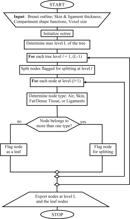
The proposed approach utilizes octrees25, 26, 27 to split the phantom volume V recursively. The octree-based approach is motivated by a desire to optimize the performance in terms of speed and computational complexity. The phantom outline S is defined by the simulated skin and chest wall (approximated by a plane). The phantom volume V consists of the simulated adipose compartments Ci, i = 1, …, K, and the fibrous Cooper’s ligaments Q, which separate the compartments from each other. The flowchart of the algorithm is presented in Fig. 1. The distribution of dense fibroglandular tissue in the phantom is then simulated by replacing the adipose with dense tissue in selected compartments.
Figure 1.
Simplified flow-chart of the octree based algorithm for breast phantom generation.
Each node of the octree is associated with a corresponding rectangular subvolume of interest B, a label indicating the simulated type of tissue or material, and a flag indicating whether the node is to be split in the next level of the tree. The recursive partitioning procedure begins with the root node, which is always flagged for splitting. The algorithm proceeds in a breadth-first fashion.28 The maximal level of the tree L is determined based upon the size of the phantom volume V and the target voxel size Δx in the phantom (i.e., the target voxel size at the end of the simulation). For each level of the tree, we generate the nodes at the next level by recursively splitting those nodes flagged for splitting. For each node at the next level, we determine whether it belongs to only one material type: the air (A), skin (S), Cooper’s ligaments (Q), or an adipose compartment (Ci). If a node belongs to a single type, it is labeled as the corresponding material type and is not split further. If, however, a node belongs to multiple types, the node is flagged for splitting. It is still necessary to label nodes that are flagged for splitting, so that the recursive partitioning process could be stopped at any selected maximal level of the tree (and restarted later if needed). If the node contains skin, it is labeled as S; otherwise, it is labeled as Q (since, in that case, a Cooper’s ligament is included among the materials in the node). The recursive partitioning procedure continues until an individual node of the tree belongs to a single type or until the maximal tree level is reached.
Simulation of the breast outline and skin
The phantom volume V and the phantom outline S are specified by the outline shape functions fm(x), fM(x), fm(x) ≥ fM(x). Specifically,
| (1) |
The breast outline is simulated with ellipsoidal surfaces, corresponding to the phantom volume vertically above and below the nipple level:
| (2) |
| (3) |
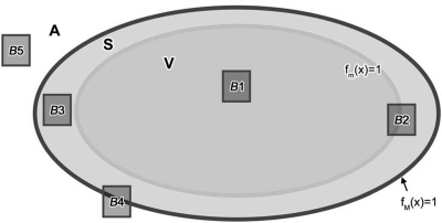
where the x-axis corresponds to the chest wall—nipple direction, the y-axis corresponds to the craniocaudal direction (i.e., vertical direction, assuming a patient in the standing position), and the z-axis corresponds to the lateral direction; (a, b′, c) and (a, b′′, c) represent the semiaxes of the ellipsoidal outline, above and below the simulated nipple point (coordinates x = a, y = 0, z = 0); and d is the thickness of the skin. The phantom exterior A, corresponding to the air (or another exterior medium depending on the simulated imaging modality), is defined as A = {x| fM(x)>1}. Subvolumes of interest B1–B5 (see Fig. 2) belong to different regions or their unions: B1⊂V; B2⊂(V∪S); B3⊂S; B4⊂(S∪A); B5⊂A. To determine whether the subvolume B (corresponding to an octree node) contains air and/or skin, we compute minima and maxima of functions fm(x), fM(x) in the subvolume (see Fig. 2). For example, if min fm(x; x∈B) > 1, max fM(x; x∈B) ≤ 1, the node belongs to the skin. If a subvolume spans more than one type of material (e.g., A and S), the node is flagged for further splitting.
Figure 2.
Two-dimensional illustration showing a cross-section of the phantom interior volume V, the outline S, and the exterior (air) A. B1–B5 represent various types of subvolumes, which are assigned to different tissue types during the recursive partitioning.
In Fig. 2, octree nodes corresponding to subvolumes B3 and B5 are leaf nodes and are labeled as S and A, respectively. The nodes corresponding to B2 and B4 are labeled as S and are subject to further splitting. The node corresponding to subvolume B1 may or may not be split further, depending on its position relative to compartment boundary (for more details see Fig. 5).
Figure 5.
Two-dimensional illustration of compartments Ci and Cj separated by a Cooper’s ligament of thickness D. Subvolumes B1.1 and B1.3 correspond to the leaf nodes of the octree (the thickness criterion satisfied), B1.1⊂Q, B1.3⊂Cj. Subvolume B1.2 is labeled with Q and is flagged for splitting.
Simulation of breast adipose compartments and Cooper’s ligaments
The simulated adipose compartments are specified by shape functions fi(x), i = 1, …, K, defined for x∈V. In the method proposed here, we have utilized compartment shape functions consistent with the quadratic decision boundaries described by a maximum a posteriori (MAP) classifier:29
| (4) |
Each shape function fi(x) is determined by a compartment seed vector si (sxi, syi, szi), a positive definite matrix , and parameters 0 ≤ qi ≤1 analog to distribution priors in MAP. Note that Eq. 4 represents a modified Mahalanobis distance29 of a point from the seed. Such defined anatomy simulation results in a variant of the 3D Voronoi diagram,30 with distances specified by Eq. 4.
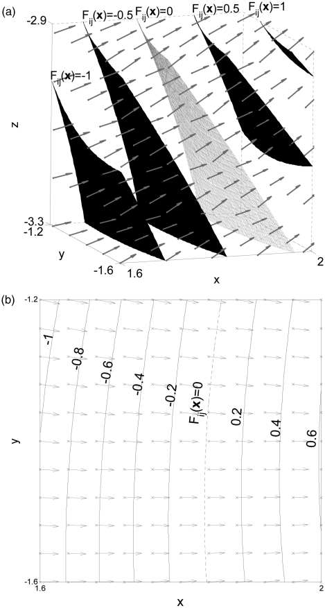
Each node of the octree is associated with a subset of shape functions fi(x). The root of the octree, in particular, is associated with all K compartment shape functions. As the algorithm proceeds, the number of shape functions associated to a node is reduced. We define the difference of the shape functions Fij(x) = fi(x) − fj(x), i ≠ j. Figure 3 illustrates isocontours and gradient vectors of Fij(x), for a choice of shape functions fi(x) and fj(x), (i ≠ j).31
Figure 3.
(a) Isosurfaces and gradient vectors (arrows) of the difference Fij(x) of shape functions inside subvolume B. The subvolume includes the midsurface between the corresponding seeds (Fij(x) = 0 [gray]); (b) Isocontours (black) and gradient vectors (arrows) of the same function at plane z = −3.1.
A point x∈B (i.e., within the subvolume corresponding to an octree node) belongs to the ith adipose compartment Ci if
| (5) |
and if the distance of x from Fij(x) = 0 is at least D/2. Otherwise, a point x∈B belongs to the Cooper’s ligament Q separating compartments Ci and Cj. This criterion assures that the targeted thickness of the simulated Cooper’s ligament is equal to D. Note that if D is smaller than or equal to the target voxel size Δx, the thickness control is not active and a region growing method is equivalent to a special case of the proposed method (see the Appendix).
To reduce the computational complexity of the algorithm, instead of evaluating Eq. 5 directly, we evaluate the following sufficient condition. A subvolume B belongs to the ith adipose compartment Ci if the distance (defined by the corresponding shape function) of the farthest point in subvolume B to the seed of the ith compartment is smaller than the shortest distance of any point in B to a seed of any other compartment. Namely, we test whether:
| (6) |
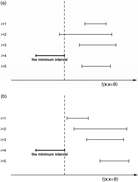
To evaluate Eq. 6, we construct intervals [min fi(x; x∈B), max fi(x; x∈B)] for the shape functions corresponding to a volume B and identify the interval corresponding to the function with the smallest minimum value (referred to as the minimum interval). If the minimum interval overlaps with any other interval, the subvolume B may contain more than one tissue type and the corresponding node is flagged for splitting. The level of the octree is incremented, and the procedure is repeated for the flagged nodes. Each child of the considered node is associated with those shape functions corresponding to the minimum interval and the interval(s) overlapping with the minimum interval [e.g., intervals #4 and #2 in Fig. 4a].
Figure 4.
Illustration of intervals of the shape function values fi(x) in a subvolume (B) of a phantom with 5 simulated compartments; x-axis corresponds to values of shape functions; y-axis corresponds to the indices of shape functions. (a) The minimum interval (#4) overlaps with #2 and the corresponding node is flagged for splitting. (b) The minimum interval does not overlap with others. The thickness criterion is evaluated based on distances of the points from B to the median surface F41(x) = 0 (since the shape function #1 has the second smallest minimum). The corresponding node is flagged for splitting if and only if the thickness criterion is not satisfied.
When the minimum interval does not overlap with any other interval, Eq. 5 is satisfied [see Fig. 4b]. In this case, the current subvolume B may include part of the compartment boundary (i.e., Cooper’s ligaments) and/or portions of at most two compartments, see Fig. 5. If the maximal distance of a subvolume from the median surface of the Cooper’s ligament is not larger than D/2 the corresponding node is a leaf of the tree and is labeled as Q. If the minimal distance of a subvolume from the median surface is larger than D/2, the corresponding node is also a leaf. The node is labeled as Ci or Cj depending on the sign of Fij(x), x∈B. Otherwise, the subvolume includes portion of a Cooper’s ligament and a portion of compartmental tissue. The node corresponding to the subvolume is flagged for further splitting and assigned a label Q.
Simulation of fibroglandular tissue distribution
We have simulated the distribution of fibroglandular (dense) tissue in the phantom by assigning some of the simulated compartments to contain dense tissue. We specify the probability pi that the ith compartment contains dense tissue, where the probability depends on the position of the compartmental seed. This is a modification from our previous simulation algorithm,2 which had a large scale ellipsoidal region with predominately fibroglandular tissue. The proposed algorithm does not create such an ellipsoidal region, thus reducing phantom’s geometric appearance and improving the realism of the simulation.
In this paper, we illustrate this approach by selecting the compartments to be filled with simulated dense tissue randomly based upon the distance of the compartmental seed to the nipple. Specifically, the probability pi is calculated as:
| (7) |
where is defined in Eq. 3, a is the x coordinate of a simulated nipple point (y = z = 0), sxi, syi, szi are coordinates of compartment seed vectors, σ is a scaling coefficient. Z is a normalization constant chosen based upon a user-specified volumetric breast density (VBD) of the phantom. (VBD is defined as the volumetric fraction of all nonadipose tissue, including the skin and Cooper’s ligaments.) We compute the volume of simulated skin and Cooper’s ligaments and determine the total needed volume of dense compartments to achieve the specified VBD. Assuming compartments of similar size, we compute the target number of dense tissue compartments by dividing the total volume of dense compartments with the average compartment volume. The normalization coefficient Z is then chosen such that the expected number of dense compartments, , is equal to this target number.
Statistical methods for assessment of the breast tissue simulation algorithm
To assess the proposed algorithm, we compared the computation time needed for phantom generation between the proposed algorithm and our previously developed region growing method.2 The simulation time was measured for phantoms with different voxel sizes. We generated 450 ml phantoms (approximately a B cup bra size32), with the ellipsoidal outline semiaxes a = b = c′′ = 5 cm, c′ = 12 cm [see Eqs. 2, 3]. The number of compartments was varied from 167 to 500. We specified the skin thickness d and the target thickness D of the Cooper’s ligaments (see Sec. 2A). The parameter d was assigned a value of 1.2 or 1.5 mm, based upon reports in the literature.33, 34 Values of D were varied from 0.1 to 0.8 mm. Note there are no explicit quantitative reports in the literature on the measured thickness of Cooper’s ligaments in clinical data. We assumed the thickness was smaller than 1 mm, as observed from subgross breast histological sections (e.g., the sections shown in Ref. 2).
For comparison, we generated phantoms with the same parameters using the region growing simulation method.2 All the simulations were implemented using MATLAB (64-bit, MathWorks, Natick, MA). Phantoms with voxel size down to 50 μm were simulated on a computer with two Intel Xeon 5650 Six Core Processors (Intel, Inc., Santa Clara, CA) working at 2.53 GHz with 128 GB RAM (1333 MHz DDR III ECC) and utilizing one core per phantom. We used MATLAB version v7.13 (R2011b).
In addition, we generated phantoms with 25 μm voxel size using a workstation with two AMD Opteron 2354 quad processors (Advanced Micro Devices, Inc., Sunnyvale, CA) working at 2.2 GHz with 64 GB RAM (667 MHz DDR II ECC), with one core per phantom, and MATLAB R2008a.
To estimate the dependence of the simulation time on the voxel size, we calculate a regression model (here referred to as a power law regression35):
| (8) |
where t represents the simulation time (in minutes), Δx the voxel size (in micrometers), β0 represents the intercept and β1 the slope in the log-log scale. Values of the slope β1 were used for comparison between the proposed and the region growing algorithm. The regression model excluded the 25 μm phantoms.
Imaging simulations
Mammographic images of the phantom are simulated using (i) a finite-element model of mammographic breast compression and (ii) simulation of the x-ray projections through the compressed phantom. The deformation model is implemented using ABAQUS (version 6.6, DS Simulia, Corp., Providence, RI) and is based upon a finite element model of breast compression proposed by Ruiter et al.36 The deformation model assumes the volume preservation of the simulated breast tissue. With that assumption, a 450 ml phantom described in Sec. 2B corresponds to a compressed phantom with the size of 20 cm in the vertical direction, 5 cm in the lateral direction, and approximately 6.5 cm in the chest wall-nipple direction. Mammographic projections of the compressed phantom are simulated assuming a monoenergetic x-ray acquisition model without scatter. The quantum noise was simulated by a random Poisson process, corresponding to the standard radiation dose of a clinical mammographic projection. The linear x-ray attenuation coefficients of the simulated tissues were selected assuming an x-ray energy of 20 keV. The simulated acquisition geometry uses a source–detector distance of 70 cm, a detector element size of 70 μm, and a 24 × 30 cm field-of-view, corresponding to the Hologic Selenia Dimensions full-field digital mammography system (Hologic, Bedford, MA).
EXPERIMENTAL RESULTS
Anthropomorphic software breast phantoms with different voxel size
Figure 6 illustrates the effect of increasing phantom resolution for an identical distribution of simulated compartments with skin thickness d = 1.5 mm and target thicknesses of Cooper’s ligaments D = 0.6 mm. The scaling coefficient in Eq. 7 was set to σ = 5. We simulated the distribution of fibroglandular (dense) tissue such that 5% of the simulated compartments contain dense tissue (which approximately corresponds to a phantom VBD of 20%).
Figure 6.
Cross-sections (upper row) and details (middle row) of three phantoms simulated using the identical positions of compartment seeds with voxel size of (a) 400 μm, (b) 100 μm, and (c) 25 μm.
Comparison with the previous region growing algorithm
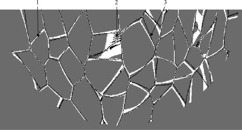
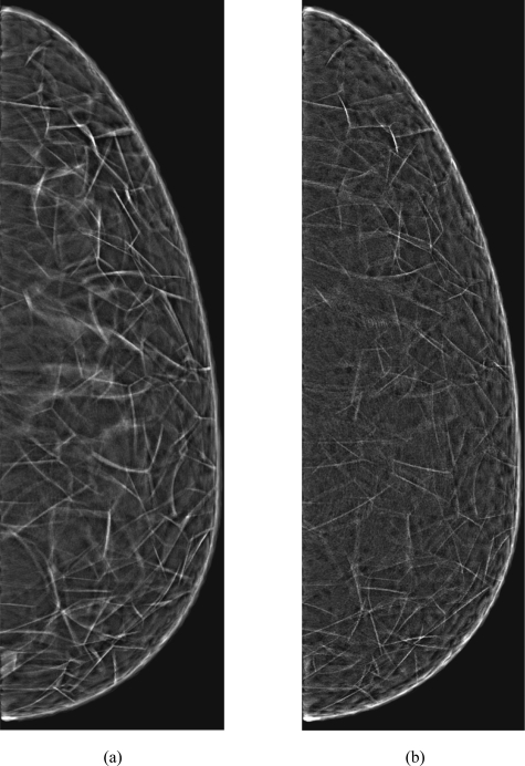
We evaluated the similarity of the results of the proposed algorithm with the previous region growing algorithm.2 Phantoms containing K = 333 compartments were simulated with 200 μm voxel size and skin thickness of d = 1.5 mm. Since the two methods differ in simulating the distribution of dense tissue, the following comparison excludes the region growing simulation of compartments in the FGT region. The proposed algorithm was run without thickness control [i.e., the decision whether a subvolume belongs to a compartment is made solely by Eq. 5] and parameters qi satisfied Eq. A8. Figure 7 contains Cooper’s ligaments generated using the region growing algorithm with no FGT region (black) superimposed upon the results of the proposed algorithm (white) in a horizontal phantom section. Synthetic mammographic projections through the compressed phantoms corresponding to Fig. 7 are shown in Fig. 8.
Figure 7.
Cooper’s ligaments generated using the region growing algorithm (black) superimposed upon the results of the proposed algorithm (white) in a horizontal phantom section. The simulated phantom contained 333 compartments and had 200 μm voxel size. (1), (2), and (3) indicate various degrees of matching between the two methods.
Figure 8.
Synthetic mammographic projections through the compressed phantoms with voxel size of 200 μm and 333 compartments simulated (a) using the proposed algorithm or (b) using the region growing algorithm.
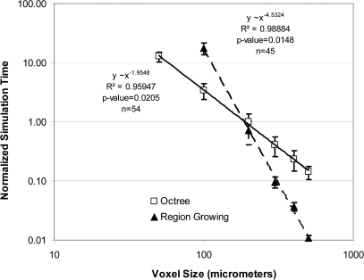
We have compared the execution time of the proposed algorithm with our previous implementation of the region growing algorithm.2 Figure 9 shows the time needed to simulate phantoms with specific resolutions (i.e., voxel sizes). The simulation was performed for phantoms generated with a target Cooper’s ligament thickness of D = 0.8 mm, skin thickness of d = 1.2 mm, and K = 167, 333, or 500 compartments. The voxel size was varied in the range of 50–500 μm for the proposed method. Figure 9 also shows the simulation times for the phantoms generated using the previous region growing algorithm with voxel sizes in the range of 100–500 μm. Using the region growing algorithm, it was not practical to simulate phantoms with voxel sizes below 100 μm, due to limitations of available computational power. We generated three phantoms for each combination of voxel size and the number of compartments, with random initialization of seed points. Figure 9 shows the estimated power regression trend lines as well as one standard deviation intervals, for measured simulation times. The regression models are computed for total of n = 45 phantoms generated by region growing and n = 54 phantoms generated using the octree approach. The figure also shows p-values for the estimated models. All displayed times are normalized by the average time achieved for 200 μm region growing phantoms.
Figure 9.
Comparison of the experimental time complexity of the proposed algorithm and previous region growing method. Shown are the values of the simulation time for phantoms at different voxel sizes. Times are normalized by the average time achieved for 200 μm region growing phantoms. Power law regression trend lines are displayed in solid (the proposed octree algorithm) and dashed (the region growing method).
When target Cooper’s ligament thicknesses was varied, the power law regression coefficients for the proposed method and the region growing method, Eq. 8, are shown in Table Table I. for simulated phantoms with K = 333 compartments. (Note that the remaining simulation parameters are the same as in Fig. 9.) The number n of samples per each regression was 18 for octree phantoms (6 voxel sizes and 3 random phantoms per voxel size) and 15 for region growing phantoms (3 random phantoms per each of 5 voxel sizes). The table also shows p-values and the values of the coefficient of determination R2 per each regression.
Table I.
The power law regression coefficients model estimated from Eq. 8 (with confidence intervals at α = 0.05) for the proposed method and for region growing, for phantoms with K = 333 compartments.
| Proposed method | Region growing | ||||
|---|---|---|---|---|---|
| Ligament thickness D (mm) | 0.1 | 0.2 | 0.4 | 0.8 | N/A |
| n | 18 | 18 | 18 | 18 | 15 |
| 4.71 ± 0.34 | 4.53 ± 0.29 | 4.63 ± 0.31 | 4.61 ± 0.19 | 10.54 ± 0.53 | |
| −2.04 ± 0.15 | −1.96 ± 0.13 | −2.01 ± 0.13 | −1.96 ± 0.08 | −4.59 ± 0.22 | |
| 0.982 | 0.9854 | 0.9845 | 0.9940 | 0.9939 | |
| P-value | 0.011 | 0.008 | 0.009 | 0.003 | 0.009 |
Phantom mammographic projections
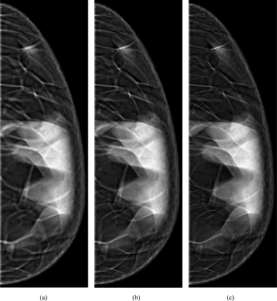
Figure 10 shows examples of synthetic phantom images. We simulated mammographic projections through the compressed phantoms generated with the same distribution of simulated adipose compartments while controlling the thickness of Cooper’s ligaments. Shown are projections through phantoms with voxel size of 200 μm and target Cooper’s ligament thickness simulated in the range of 400–1200 μm. The number and distribution of simulated compartments are the same as in Sec. 3B.
Figure 10.
Synthetic mammographic projections through the compressed phantoms with voxel size of 200 μm and thicknesses of simulated Cooper’s ligaments of (a) 1200 μm, (b) 800 μm, and (c) 400 μm.
DISCUSSION
We have developed a novel method for generating software breast phantoms. Based upon the use of recursive partitioning and octrees, the method provides a very efficient way for generating phantom with high spatial resolution. As illustrated in Fig. 5c with the current computational power available, the novel method allows simulation of breast anatomical details down to a size of 25 μm/voxel.
Time complexity
Our experimental results, Fig. 9, indicate that the elapsed time of the proposed method increases approximately as 1/Δx2. Using the t-test,35 we cannot reject hypothesis |β1| = 2 (at significance level α = 0.05), and there is strong statistical evidence that |β1|< 3 (α = 1 × 10⁻⁶). By contrast, for the region growing method, the t-test indicated that the elapsed time increases significantly faster than 1/Δx3 (α = 1 × 10⁻⁶). Hence, there is strong statistical evidence that the asymptotical time complexity37 of the proposed method is lower than the complexity of region growing method.
Note that the regressions in Fig. 9 were performed for phantoms with different numbers of compartments K. The dependence of the elapsed time on the number of compartments will be more thoroughly examined in our future work.
The results in Fig. 9 were shown for a single target thickness (0.8 mm). In Table Table I., we explore the influence of the target thickness on elapsed simulation time. All the estimated models were statistically significant (p-value < 0.02). Results from Table Table I. indicate that the slope of the power regression model was not influenced by the specified target thickness of simulated Cooper’s ligaments for a particular number of compartments (K = 333) (the test for comparison of slopes of regression lines38 resulted in p-value = 0.7218). The results from Table Table I. on region growing, estimated on phantoms with 333 compartments, were consistent with the results from Fig. 9 (that are estimated on phantoms with 167, 333, and 500 compartments).
Figure 9 shows that the proposed method is faster than our previous method (based upon region growing), for phantom voxel size smaller than 200 μm. For example, the region growing takes about 4–8 days to generate a 450 ml phantom with voxel size of 100 μm. The proposed method can generate 50 μm voxel size phantom within a comparable time (of 3–5 days) on the same platform. In addition, the proposed method makes the simulation of very high resolution phantoms tractable. As a demonstration of this, we simulated one phantom with Δx = 25 μm, which took 12.5 days (on a workstation with two AMD Opteron 2354 quad processors). The region growing algorithm would require in excess of 1000 CPU days on the same platform (based on extrapolating the regression results from Fig. 9).
The proposed method provides tractable simulation at the voxel size comparable to the adipocyte size.39 This opens possibilities for novel applications of the software phantoms, e.g., simulation of histological specimen of the breast tissue, simulation of breast tissue physiological processes at the cellular level, etc. Although affordable, such a level of simulated detail currently requires considerable memory size. To alleviate this issue, further efficiency gains are possible by increasing the resolution only within selected phantom subvolumes of interest (e.g., for simulated lesions). Namely, the maximal level L of the octrees does not need be constant but may depend on the spatial location of nodes. Hence, the proposed methods can be utilized to simulate finer details in particular regions of phantom that may be of special interest for analysis. Since the nodes of the subtrees corresponding to children of a particular octree node can be processed independently, the algorithm is suitable for parallelization by implementation on platforms with multiple processors/cores and/or on clusters. Also, additional acceleration is achievable by using a graphical processing unit (GPU) based implementation.40, 41, 42
Thickness control of Cooper’s ligaments
Figure 10 shows synthetic mammographic projections through phantoms with the same composition but three different thicknesses of simulated Cooper’s ligaments; the changes in ligament thickness are visible in the synthetic images. An advantage of the proposed method is that a phantom with a smaller voxel size can be generated using a larger voxel size phantom, instead of starting the simulations all over again. When the phantom voxel size was 300 μm or smaller, we observed that thickness of Cooper ligaments remained practically constant, indicating that the thickness control was achieved. Further increase of resolution led to smoother boundaries of the Cooper ligaments.
Thickness control depends on our ability to determine distance. Although the proposed method is demonstrated to be useful for simulating Cooper’s ligaments of a desired thickness, it could be further improved. Namely, Fig. 6 illustrates “indentations” in the simulated ligaments’ boundaries that are, albeit to a lesser extent, present even at the finest simulated resolution (25 μm). Further modifications of the algorithm that approximate the distance between the median surface of the Cooper’s ligaments and the subvolumes may improve the shape of ligaments by avoiding the indentations.
Trade-off between time complexity and model precision
When deciding whether to continue with subvolume splitting, we test a sufficient condition Eq. 6; this approach is computationally simple, thereby contributing to the overall efficiency of the algorithm. However, the tested condition is sufficient but not necessary. Hence, each node that needs to be split will be identified as such, but some nodes that may not require splitting will nevertheless be split as well. Hypothetically, it could be possible to introduce more selective and specific conditions in the splitting criterion. This could lead to fewer unnecessary splits; but, in turn, the time for each particular splitting would be larger. Achieving a good trade-off between the simplicity and selectivity/specificity of the node splitting criterion is part of our work in progress.
Additional control of simulated anatomical features
In Sec. 2A3, we described a method for simulation of dense tissue regions in the phantom (as illustrated in Fig. 10). More realistic distributions of fibroglandular tissue can be achieved by modifying the choice of the probability pi that the ith compartment contains dense tissue, instead of using Eq. 7.
The described simulation method provides for skin thickness control, as described by Eqs. 2, 3. These equations, however, do not guarantee a constant skin thickness over the whole phantom surface. This issue can be corrected by modifying function fM from Eq. 3 to represent a surface at a prespecified distance from the inner surface specified by function fm, Eq. 2. Alternatively, thickness control mechanisms, similar to those adopted in Sec. 2A2 can be used. However, these modifications would reduce the efficiency of the algorithm.
Qualitative comparison with region growing algorithm
The underlying mathematics of the region growing method and the proposed algorithm is similar, as shown in the Appendix. As a consequence, the region growing method and the proposed method give similar results. Large overlap of ligaments simulated using the two methods [denoted by (1)] is evident in Fig. 7. The simulated phantoms are, however, not identical. The thickness of Cooper’s ligaments differs between the two methods. In addition, the region-growing algorithm can result in a characteristic zigzag pattern [denoted by (2) in Fig. 7], and there are slight shifts between Cooper’s ligaments generated using the two methods [denoted by (3) in Fig. 7].
A visual comparison of mammographic projections synthesized using the phantoms generated with the two methods (Fig. 8) indicates very similar appearance of simulated parenchymal pattern. The observed differences include more prominent linear features in the image synthesized using the proposed method and a more noisy appearance of the images generated by the region growing.
These differences can be explained by the fact that the region growing is based on determining positions of voxels belonging to compartments, with Cooper’s ligaments formed at the boundary of neighboring compartments. The octree approach simulates Cooper’s ligaments directly, while the compartment labels are assigned as side products of the process. Due to the nature of region growing, Cooper’s ligaments in the AT region are always one voxel thick. In contrast, the ligament thickness in the proposed algorithm is controlled. As a consequence, the thickness of Cooper’s ligaments simulated using the proposed method is effectively larger as compared to region growing.
The zigzag pattern in phantoms generated by region growing [denoted by (2) in Fig. 7] stems from sequential character of voxel labeling. Such a sequential labeling cannot accurately render a smooth surface of Cooper’s ligaments. This zigzag pattern also introduces additional noise artifacts in synthetic phantom projections [Fig. 8a]. The octree method effectively eliminates this noise, thus yielding an improved realism of synthetic images. The sequential labeling also prevents efficient parallelization of region growing. On the other hand, the parallelization of the proposed algorithm is straightforward, as discussed in Sec. 4A.
Slight mismatch between Cooper’s ligaments [denoted by (3) in Fig. 7] can be explained by implementation details of the region growing algorithm. Namely, the equivalence between the two methods derived in the Appendix holds only if the virtual time (τ) in the region growing algorithm is continuous. Practically, this time is discretized resulting in the quantized positions of calculated boundaries between compartments, causing the observed mismatch.
CONCLUSIONS
A novel algorithm for computing anthropomorphic software breast phantoms has been described, providing substantial improvement in the efficiency of generating phantoms with a small voxel size. This design feature is of particular importance in virtual clinical trials requiring large number of phantoms. The proposed methodology also allows for scalability in phantom generation and better quality of the simulated phantom images. These improvements are especially important for the use of phantom images generated using realistic detector resolutions.
ACKNOWLEDGMENTS
This work was supported in part by the U.S. Department of Defense Breast Cancer Research Program (HBCU Partnership Training Award No. BC083639), the U.S. National Institutes of Health (R01 Grant No. CA154444), the U.S. National Science Foundation (Research Grant No. IIS-0916690 and CREOSA Grant No. HRD-0630388), and the U.S. Department of Defense/Department of Army (45395-MA-ISP, Grant No. 54412-CI-ISP). The authors would like to thank Ms. Beverly Lau from the University of Chicago for helpful discussions about improving the previous version of the phantom, Dr. Fengshan Liu from Delaware State University for providing support, Ms. Samantha McDaniel for help with figures, and Ms. Susan Ng from Real-Time Tomography (Villanova, PA) for processing the simulated projection images. This work has been presented in part at the 2011 Joint AAPM/COMP Meeting, Vancouver, Canada.
NOMENCLATURE
- A =
label for voxels representing air—or another exterior medium depending on the simulated imaging modality
- B =
phantom subvolumes, corresponding to octree nodes at various levels
- Ci, i = 1, …, K =
simulated tissue compartments
- D =
thickness of the simulated Cooper’s ligaments
- Fij(x) =
difference of the compartment shape functions fi(x) and fj(x)
- K =
number of simulated compartments
- N =
simulated nipple point
- Q =
label for voxels representing fibrous Cooper’s ligaments
- R2 =
goodness-of-fit of the regression model
- Ri =
eigenvectors of a positive definite matrix specifying shape functions and region growing
- S =
label for voxels representing the phantom outline, i.e., a simulated layer of skin
- V =
phantom volume
- Z =
normalization constant based upon the desired overall phantom glandularity
- a =
distance of the simulated nipple point from the chest wall
- b′ =
vertical phantom dimension measured above the nipple level
- b″ =
vertical phantom dimension measured below the nipple level
- c =
half of the uncompressed phantom thickness
- d =
thickness of the simulated skin
- ei =
ellipsoid containing a seed and a nipple at region growing algorithm
- fi(x), i = 1, …, K =
compartment shape functions
- fM(x) =
shape function defining the outer surface of the simulated skin layer
- fm(x) =
shape function defining the inner surface of the simulated skin layer
- kai, kbi, kci =
proportionality coefficients for region growing growth of ellipsoids
- k =
shrinkage coefficient at region growing algorithm
- l = 1, …, (L −1) =
Levels of the octree
- =
axis vector of local ellipsoid in region growing algorithm
- pi =
probability that the ith simulated compartment contains dense tissue
- qi =
parameters of the proposed algorithm (analog to distribution priors in MAP classification algorithm)
- r1,i, r2,i =
axis ratios of region growing algorithm
- spi =
growing speed of region growing algorithm
- (sxi, syi, szi) =
coordinates of the ith compartment seed vector
- t =
phantom simulation time (min).
- =
axis vector of local ellipsoid in region growing algorithm
- =
axis vector of local ellipsoid in region growing algorithm
- x =
coordinate of a point within the phantom (or the exterior medium)
- Δx =
phantom voxel size (μm)
- α =
significance level
- β0, β1 =
intercept and slope of the log-log scale regression model, respectively.
- σ =
scaling coefficient for dense tissue modeling
- τ, τi =
virtual time of region growing
- Λi =
eigenvalues of a positive definite matrix specifying shape functions and region growing
- =
positive definite matrix specifying a shape function and a local ellipsoid at region growing algorithm
APPENDIX I: REGION GROWING ALGORITHM AS A SPECIAL CASE OF THE PROPOSED APPROACH
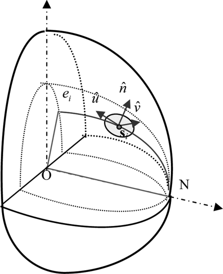
In the region growing algorithm,2 each compartment of adipose tissue in the AT region is assigned an ellipsoid. The ellipsoid is centered at a randomly chosen seed point and its semiaxes grow proportional to a virtual time τ ≥ 0. Each voxel is labeled corresponding to a seed of the ellipsoid that first reaches the voxel during the growing procedure. More formally, an ellipsoid centered at the point specified by a seed vector si =[sxi, syi, szi]T has semiaxes kaiτ, kbiτ, kciτ, determined by the growing speeds spi and the axis ratios r1,i, r2,i:
| (A1) |
The orientations of the ellipsoid semiaxes are specified by column vectors defined as follows. Consider an ellipsoid ei centered at the origin O(0,0,0) and containing point si and a nipple N(a,0,0). The ellipsoid is specified by:
| (A2) |
where k is the shrinkage coefficient defined as:
| (A3) |
We define vector as a unit normal vector on the ellipsoid ei at si. Vector is a normal unit vector of the plane ONsi, while , see Fig. 11.
Figure 11.
Illustration of ellipsoid orientation for region growing (modified from Ref. 2).
Following this formalism, points x at an ellipsoid centered at si at a specific virtual time τi satisfy
| (A4) |
where is a positive definite matrix with eigenvalues and column eigenvectors , , such that:
| (A5) |
Since, in the region growing algorithm, the voxel is labeled according to the ellipsoid that reaches the voxel first, the compartment label j generated by the region growing algorithm satisfies
| (A6) |
Due to Eq. A6, compartment boundaries in the region growing represent Voronoi diagrams30 with respect to the Mahalanobis distance.28 On the other hand, it is easy to demonstrate that:
| (A7) |
where functions fi(x) are defined by Eq. 4, are defined by Eq. A5 and
| (A8) |
Note that arg minifi(x) implies Eq. 5. Hence, the region assignment in the region growing algorithm reduces to compartment assignment. In the region growing algorithm, there is no explicit thickness control of Cooper’s ligaments (i.e., the thickness of the ligaments depends only on the target voxel size). Hence, the result of a theoretic region growing algorithm is equivalent to a special case of the proposed algorithm when thickness control is not applied (e.g., when a minimal thickness is smaller than a target voxel size Δx). Note that in the actual implementation of region growing,2 the virtual time is discrete, which may lead to slight discrepancy of labeling w.r.t. Eq. A6.
References
- Bakic P. R., Albert M., Brzakovic D., and Maidment A. D. A., “Mammogram synthesis using a 3D simulation. I. Breast tissue model and image acquisition simulation,” Med. Phys. 29(9), 2131–2139 (2002). 10.1118/1.1501143 [DOI] [PubMed] [Google Scholar]
- Bakic P. R., Zhang C., and Maidment A. D. A., “Development and characterization of an anthropomorphic breast software phantom based upon region-growing algorithm,” Med. Phys. 38(6), 3165–3176 (2011). 10.1118/1.3590357 [DOI] [PMC free article] [PubMed] [Google Scholar]
- Taylor P. and Owens R., “Simulated mammography using synthetic 3D breasts,” in 4th International Workshop on Digital Mammography, edited by Karssemeijer N. (Kluwer, Nejmegen, The Netherlands, 1998), pp. 283–290.
- Bliznakova K., Bliznakov Z., Bravou V., Kolitsi Z., and Pallikarakis N., “A three-dimensional breast software phantom for mammography simulation,” Phys. Med. Biol. 48(22), 3699–3719 (2003). 10.1088/0031-9155/48/22/006 [DOI] [PubMed] [Google Scholar]
- Ma A. K. W., Gunn S., and Darambara D. G., “Introducing DeBRa: A detailed breast model for radiological studies,” Phys. Med. Biol. 54, 4533–4545 (2009). 10.1088/0031-9155/54/14/010 [DOI] [PubMed] [Google Scholar]
- Bliznakova K., Suryanarayanan S., Karellas A., and Paiilikarakis N., “Evaluation of an improved algorithm for producing realistic 3D breat software phantoms: Application for mammography,” Med. Phys. 37(11), 5604–5617 (2010). 10.1118/1.3491812 [DOI] [PMC free article] [PubMed] [Google Scholar]
- Reiser I. and Nishikawa R. M., “Task-based assessment of breast tomosynthesis: Effect of acquisition parameters and quantum noise,” Med. Phys. 37(4), 1591–1600 (2010). 10.1118/1.3357288 [DOI] [PMC free article] [PubMed] [Google Scholar]
- Chen B. et al. , “An anthropomorphic breast model for breast imaging simulation and optimization,” Acad. Radiol. 18(5), 536–546 (2011). 10.1016/j.acra.2010.11.009 [DOI] [PubMed] [Google Scholar]
- Li C. M., Segars W. P., Tourassi G. D., Boone J. M., and J. T.DobbinsIII, “Methodology for generating a 3D computerized breast phantom from empirical data,” Med. Phys. 36(7), 3122–3131 (2009). 10.1118/1.3140588 [DOI] [PMC free article] [PubMed] [Google Scholar]
- Hoeschen C., Fill U., Zankl M., Panzer W., Regulla D., and Dohring W., “A high resolution voxel phantom of the breast for dose calculations in mammography,” Radiat. Prot. Dosim. 114(1–3), 406–409 (2005). 10.1093/rpd/nch558 [DOI] [PubMed] [Google Scholar]
- O’Connor J. M., Das M., Didier C., Mah D. M., Glick S. J., “Comparison of two methods to develop breast models for simulation of breast tomosynthesis and CT,” in Digital Mammography (IWDM) Lecture Notes in Computer Science, edited by Krupinski E. A. (Springer-Verlag, Berlin, Heidelberg, 2008), Vol. 5116, pp. 417–425. [Google Scholar]
- Lee C. H. et al. , “Breast cancer screening with imaging: Recommendations from the Society of Breast Imaging and the ACR on the use of mammography, breast MRI, breast ultrasound, and other technologies for the detection of clinically occult breast cancer,” J. Am. Coll. Radiol. 7(1), 18–27 (2010). 10.1016/j.jacr.2009.09.022 [DOI] [PubMed] [Google Scholar]
- Zhang C., Bakic P. R., and Maidment A. D. A., “Development of an anthropomorphic breast software phantom based on region growing algorithm,” in SPIE Medical Imaging: Visualization Image-guided Procedures, and Modeling, edited by Sonka M. and Manduca A. (SPIE, San Diego, CA, 2008), Vol. 6918. [Google Scholar]
- Bakic P. R., Ng S., Ringer P., Carton A.-K., Conant E. F., and Maidment A. D. A., “Validation and optimization of digital breast tomosynthesis reconstruction using an anthropomorphic software breast phantom,” in SPIE Medical Imaging: Physics of Medical Imaging, edited by Samei E. and Pelc N. (SPIE, San Diego, CA, 2010), Vol. 7622. [Google Scholar]
- Bakic P. R., Ringer P., Kuo J., Ng S., and Maidment A. D. A., “Analysis of geometric accuracy in digital breast tomosynthesis reconstruction,” in Digital Mammography (IWDM), Lecture Notes in Computer Science, edited by Martí J., Oliver A., Freixenet J., and Martí R. (Springer-Verlag, Berlin Heidelberg, 2010), Vol. 6136, pp. 62–69. [Google Scholar]
- Bakic P. R.et al. , “Comparison of 3D and 2D breast density estimation from synthetic ultrasound tomography images and digital mammograms of anthropomorphic software breast phantoms,” in SPIE Medical Imaging: Physics of Medical Imaging, edited by Pelc N. J., Samei E., and Nishikawa R. M. (SPIE, Lake Buena Vista, FL, 2011), Vol. 7961. [Google Scholar]
- Lau B. A., Bakic P. R., Reiser I., Carton A.-K., Maidment A. D. A., and Nishikawa R. M., “An anthropomorphic software breast phantom for tomosynthesis simulation: Power spectrum analysis of phantom reconstructions,” Med. Phys. 37, 3473 (2010). 10.1118/1.3469567 [DOI] [Google Scholar]
- Bakic P. R., Lau B., Carton A.-K., Reiser I., Maidment A. D. A., and Nishikawa R. M., “An anthropomorphic software breast phantom for tomosynthesis simulation: Power spectrum analysis of phantom projections,” in Digital Mammography (IWDM), Lecture Notes in Computer Science, edited by Martí J., Oliver A., Freixenet J., and Martí R. (Springer-Verlag, Berlin, Heidelberg, 2010), Vol. 6136, pp. 452–458.
- Kontos D., Zhang C., Ruiter N. V., Bakic P. R., and Maidment A. D. A., “Evaluating the effect of tomosynthesis acquisition parameters on image texture: A study based on an anthropomorphic breast tissue software model,” in Digital Mammography (IWDM), Lecture Notes in Computer Science, edited by Krupinski E. A. (Springer-Verlag, Berlin, Heidelberg, 2008), Vol. 5116, pp. 681–688. [Google Scholar]
- Young S., Park S., Anderson K., Badano A., Myers K. J., and Bakic P. R., “Estimating DBT performance in detection tasks with variable-background phantoms,” in SPIE Medical Imaging: Physics of Medical Imaging, edited by Samei E. and Hsieh J. (SPIE, Lake Buena Vista, FL, 2009), Vol. 7258. [Google Scholar]
- Carton A.-K., Derand H., Ullberg C., Bakic P. R., and Maidment A. D. A. “Development of a 3D physical anthropomorphic breast phantom,” In Tomosynthesis Imaging Symposium 2009: Frontiers in Research and Clinical Applications, 2009, Durham, NC: (2009).
- Carton A.-K., Bakic P. R., Ullberg C., and Maidment A. D. A., “Development of a 3D high-resolution physical anthropomorphic breast phantom,” in SPIE Medical Imaging: Physics of Medical Imaging, edited by Samei E. and Pelc N. J. (SPIE, San Diego, CA, 2010), Vol. 7622. [Google Scholar]
- Carton A.-K., Bakic P. R., Ullberg C., Derand H., and Maidment A. D. A., “Development of a physical 3D anthropomorphic breast phantom,” Med. Phys. 38(2), 891–896 (2011). 10.1118/1.3533896 [DOI] [PMC free article] [PubMed] [Google Scholar]
- Breiman L., Classification and Regression Trees (Chapman and Hall, London, 1984). [Google Scholar]
- Meagher D., “Geometric modeling using octree encoding,” Comput. Graph. Image Process. 19, 129–147 (1981). 10.1016/0146-664X(82)90104-6 [DOI] [Google Scholar]
- Badal A., Kyprianou I., Badano A., Myers K. J., and Sempau J., “Monte Carlo package for simulating radiographic images of realistic anthropomorphic phantoms described by triangle meshes,” in Physics of Medical Imaging, 2007, edited by Hsieh J. and Flynn M. J. (SPIE, San Diego, CA, 2007). [Google Scholar]
- Megalooikonomou V., Kontos D., Pokrajac D., Lazarevic A., and Obradovic Z., “An adaptive partitioning approach for mining discriminant regions in 3D image data,” J. Intell. Inf. Syst. 31, 217–242 (2008). 10.1007/s10844-007-0043-2 [DOI] [Google Scholar]
- Moore E., “The shortest path through a maze,” in International Symposium on the Theory of Switching, 1959. (Harvard University, Cambridge, MA, 1959), pp. 285–292.
- Duda R. O., Hart P. R., and Stork D. G., Pattern Classification, (John Wiley & Sons, Inc., New York, 2001). [Google Scholar]
- Okabe A., Boots B., Sugihara K., and Chiu S. N., Spatial Tessellations—Concepts and Applications of Voronoi Diagrams, 2nd ed. (John Wiley & Sons, New York, 2000). [Google Scholar]
- The functions fi(x) and fj(x) are specified by the seeds: si = [1.0432 −1.4242 −3.3089]T, sj = [2.5618 −1.2814 −2.8567]T, priors qi = qj = 1/333, and positive definite matrices: ∑i-1=[1.603-0.14763-0.063546-0.147633.3497-1.7409-0.063546-1.74096.6449],∑j-1=[4.0088-1.0346-0.4641-1.03465.62391.1105-0.46411.11053.6465]
- Ringberg A., Bageman E., Rose C., Ingvar C., and Jernstrom H.. “Of cup and bra size: Reply to a prospective study of breast size and premenopausal breast cancer incidence,” Int. J. Cancer 119(9), 2242–2243 (2006). 10.1002/ijc.22104 [DOI] [PubMed] [Google Scholar]
- Pope T. L., Read M. E., Medsker T., Buschi A. I., and Brenbridge A. N., “Breast skin thickness: Normal range and cause of thickening shown on film-screen mammography,” J. Can. Assoc. Radiol. 35(4), 365–368 (1984). [PubMed] [Google Scholar]
- Ulger H., Erdogan N., Kumanlioglu S., and Unue E., “Effect of age, breast size, menopausal and hormonal status on mammographic skin thickness,” Skin Res. Technol. 9(3), 284–289 (2003). 10.1034/j.1600-0846.2003.00027.x [DOI] [PubMed] [Google Scholar]
- Devore J. L., Probability and Statistics for Engineering and the Sciences (Brooks/Cole, Belmont, CA, 2008). [Google Scholar]
- Ruiter N. V., Stotzka R., Mueller T. O., Gemmeke H., Reichenbach J. R., and Kaiser W. A., “Model-based registration of x-ray mammograms and MR images of the female breast,” IEEE Trans. Nucl. Sci. 53(1), 204–211 (2006). 10.1109/TNS.2005.862983 [DOI] [Google Scholar]
- Cormen T. H., Leiserson C. E., Rivest R. L., and Stein C., Introduction to Algorithms, 2nd ed. (MIT, Cambridge, MA, 2001). [Google Scholar]
- Armitage P., Berry G., and Matthews J. N. S., Statistical Methods in Medical Research (Blackwell Science, Malden, MA, 2001). [Google Scholar]
- Jernas M. et al. , “Separation of human adipocytes by size: hypertrophic fat cells display distinct gene expression,” FASEB J. 20, E832–E839 (2006). 10.1096/fj.05-5678fje [DOI] [PubMed] [Google Scholar]
- Badal A. and Badano A., “Accelerating Monte Carlo simulations of photon transport in a voxelized geometry using a massively parallel graphics processing unit,” Med. Phys. 36(11), 4878–4880 (2009). 10.1118/1.3231824 [DOI] [PubMed] [Google Scholar]
- Kuo J., Ringer P., Fallows S. G., Ng S., Bakic P. R., and Maidment A. D. A., “Dynamic reconstruction and rendering of 3D tomosynthesis images,” in SPIE Medical Imaging: Physics of Medical Imaging, edited by Pelc N., Samei E., and Nishikawa R. M. (SPIE, Lake Buena Vista, FL, 2011), Vol. 7961. [Google Scholar]
- Chui J. H., Pokrajac D. D., Maidment A. D. A., and Bakic P. R., “Roadmap for efficient parallelization of breast anatomy simulation,” in SPIE Medical Imaging: Physics of Medical Imaging, edited by Pelc N. and Nishikawa R. M. (SPIE, San Diego, CA: ), Vol. 8313. [Google Scholar]


