Automated Recognition of Robotic Manipulation Failures in High-throughput Biodosimetry Tool

Abstract

A completely automated, high-throughput biodosimetry workstation has been developed by the Center for Minimally Invasive Radiation Biodosimetry at Columbia University over the past few years. To process patients’ blood samples safely and reliably presents a significant challenge in the development of this biodosimetry tool. In this paper, automated failure recognition methods of robotic manipulation of capillary tubes based on a torque/force sensor are described. The characteristic features of sampled raw signals are extracted through data preprocessing. The twelve-dimensional (12D) feature space is projected onto a two-dimensional (2D) feature plane by the optimized Principal Component Analysis (PCA) and Fisher Discrimination Analysis (FDA) feature extraction functions. For the three-class manipulation failure problem in the cell harvesting module, FDA yields better separability index than that of PCA and produces well separated classes. Three classification methods, Support Vector Machine (SVM), Fisher Linear Discrimination (FLD) and Quadratic Discrimination Analysis (QDA), are employed for real-time recognition. Considering the trade-off between error rate and computation cost, SVM achieves the best overall performance.

1. Introduction

High speed and efficient automation of biodosimetric assays for triage is becoming a top priority for homeland security [1]. A robotically-based Rapid Biodosimetry Tool (RABiT) has been developed [2], which automates two mature assays (micronucleus and γ-H2AX assay) for triage following radiation exposure and is able to process 6,000 samples/day. Robust mechanical and electrical designs are introduced to improve the RABiT’s reliability to avoid process failures as many as possible. However, there still exists 0.5 to 1.0 percent manipulation-related failure rate because plastic (PVC) capillaries are easily distorted. Therefore, it is necessary to develop effective fault diagnosis capability to recover the RABiT from failures and bring the process back to an in-control state. It is also helpful for the RABiT to take immediate remedial actions to save samples, such as blood, lymphocytes, etc. in the capillary tubes. Otherwise lost or damaged samples may lead to a delay in treatment of severely irradiated patients.

Explicit model-based expert systems in a complex robot system [3] need more elaborate models for probability elicitation to improve quantitative modeling and better intelligent diagnosis, while the failure recognition methods proposed in this paper are based on experimental raw data from sensors. The first step is to search for the most characteristic features from available large amount of historical data (training data) [4]. Many statistic techniques for analyzing these massive datasets have been developed including Principal Component Analysis (PCA) and Fisher Discriminant Analysis (FDA) [5]. A methodology to extract features combining PCA with wavelet analysis was proposed [6]. FDA provides an optimal lower dimensional representation in terms of discriminating among classes of data [7], where for fault diagnosis, each class corresponds to data collected during a specific known fault. Although FDA has been heavily studied in the pattern classification literature and is only slightly more complex than PCA, its use for analyzing biodosimetry assay process is not reported. It is expected that FDA should outperform PCA when the primary goal is to discriminate among faults.

The following step after obtaining the characteristic features is to search for optimized classifiers to discriminate feature data. The Bayesian decision rule assigns a pattern to the class with the maximal posterior probability. Commonly used parametric models are multivariate Gaussian distributions for continuous features, binomial distributions for binary features, and multi-normal distributions for integer-valued (and categorical) features. For Gaussian distributions, if the covariance matrices for different classes are assumed to be identical, then the Bayesian rule provides a linear decision boundary. On the other hand, if the covariance matrices are different, the resulting Bayesian rule provides a quadratic decision boundary. Another category of classifiers is to construct decision boundaries directly by optimizing certain error criterion. A classical example of this type of classifier is Fisher Linear Discriminant (FLD) that minimizes the mean squared error (MSE) between the classifier output and the desired labels. Support Vector Machine (SVM) is among the most robust and successful classification algorithms [8] by maximizing the margin (distance from the separating hyperplane to the nearest example). SVM performs well when applied to problems which have a small sample, are nonlinear and high dimensional. In particular, SVM exhibits the maximum generalization ability even when the samples are few. It is with this advantage that SVM has been successfully applied to many fields including classification recognition, regression analysis and forecast [9]. The basic SVM supports only binary classification, but extensions have been proposed to handle the multiclass classification case as well [10].

This paper begins with the classification of the failures of manipulating PVC capillaries. Two feature extraction methods: PCA and FDA are implemented and compared to construct two-dimensional (2D) feature planes from twelve-dimensional (12D) features. FDA yields a better separability index than that of PCA and produces well separated classes. SVM, FLD and QDA are employed to search for optimal classifiers offline and online fault recognition. Considering the trade-off between error rate and computation cost, SVM achieves the best overall performance.

2. Description of a High-throughput Biodosimetry Tool

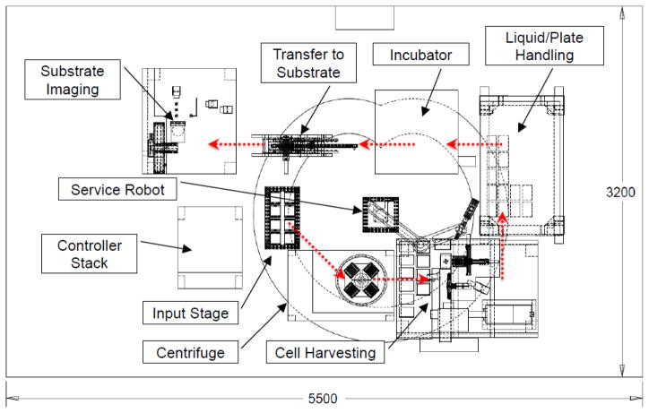
Figure 1 presents the layout and the sample flow direction of the biodosimetry workstation [2]. Patients’ blood is collected in PVC capillaries and fed into the RABiT at the input stage. After a five-minute centrifugation, lymphocytes are separated from Red Blood Cells (RBC). In the cell harvesting module, lymphocytes are extracted from individual capillaries and dispensed into a micro-well plate with membrane at the bottom of each well. The plate is transferred to a liquid/plate handling system (including an incubator) where filter reagents specific for each assay are sequentially dispensed. Following the completion of the assays, the underdrains are removed from the plate and the membranes are peeled off and sealed between two adhesive transparent sheets (substrate) at the Transfer to Substrate (TTS) module. Finally, the substrate is delivered to the substrate imaging module, where dedicated imaging hardware and software measure yields of micronuclei or γ-H2AX, which are already well-characterized quantifiers for radiation exposure.

Figure 1.

Layout of the rapid biodosimetry tool.

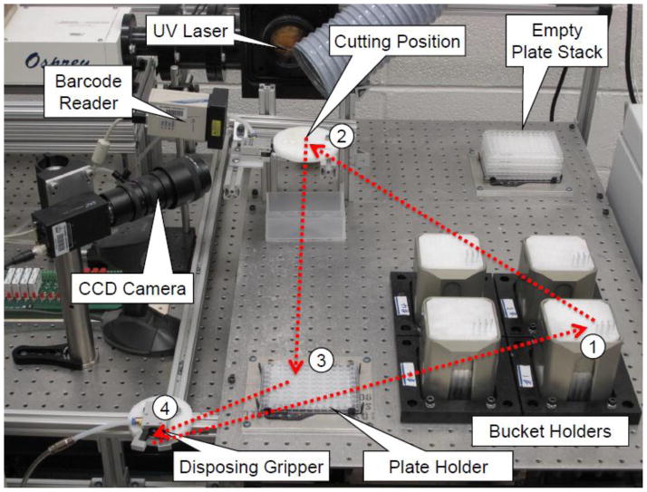
Most of robotic manipulation actions are taken place in the cell harvesting module (Figure 2). Initially the service robot transfers centrifuged buckets from the centrifuge to the bucket holders, and then loads an empty micro-well plate from the plate stack to the plate holder. The service robot repeats the same sequence of manipulating actions by 96 times till 96 wells of the micro-well plate are filled with lymphocytes. In each of the manipulating sequences, the capillary gripper mounted on the end arm of the service robot is to pick up individual capillaries first and then carry the capillary to the cutting position where the laser beam is fired to cut the tube. At the cutting position, a CCD camera is used to identify the cutting position and a barcode reader is used to identify the ID of the sample. Then the bottom part of the capillary containing the RBC pellet is disposed, while the upper part is moved above the micro-well plate to dispense the lymphocytes in the micro-well plate pneumatically. Finally, the empty upper part of the tube is pulled out from the collet of the capillary gripper by the tube disposing gripper. When the micro-well plate is full, the service robot will transfer the plate to the liquid/plate handling module.

Figure 2.

Prototype and processing sequence of the cell harvesting module (➀: pick up a capillary; ➁: detect separation band, read barcode, cut the capillary; ➂: dispense lymphocytes; ➃: dispose the empty capillary).

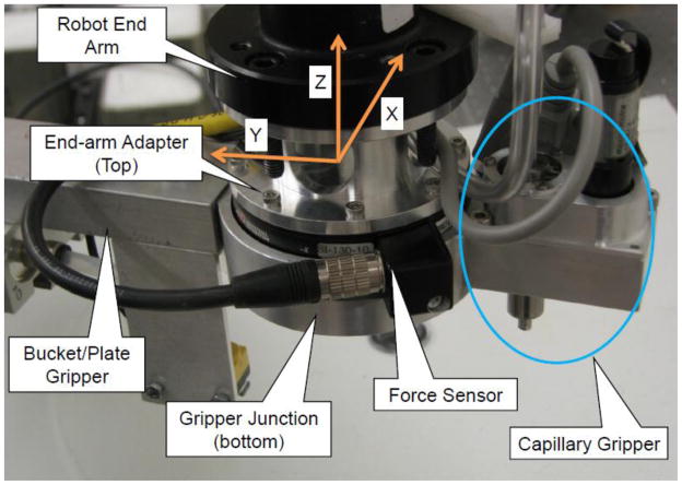
All failure recognition and recovery in this paper are based on the data from a force/torque sensor with the setup shown in Figure 3. The top surface of the sensor is attached to the end arm of the service robot. Its bottom is connected with a gripper junction, where the capillary gripper is mounted. The sensor measures the forces and torques in the Cartesian coordinates denoted as (F_x, F_y, F_z, T_x, T_y, T_z).

Figure 3.

Force/torque sensor mounting and its Cartesian coordinates.

3. Overall Scheme of Recognition and Recovery

While the paper is focused on the recognition aspect, its connection with the monitoring aspect and recovery aspect are also briefly described below.

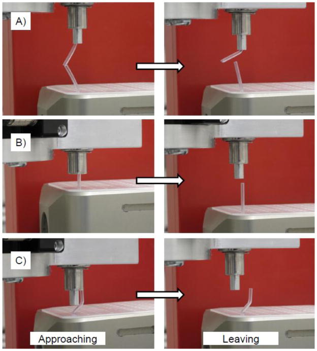
The maximum force on the Z axis (F_zmax) during picking up a capillary is used to monitor if the robotic manipulation is successful or failed. In the normal operation, F_zmax has the range from 5.43 N to 6.13 N. While in the failed operation, a spike of force is sensed. Figure 4 shows three typical failures of picking up capillaries and their manipulation steps (approaching to the picking position for a new capillary, leaving from the picking position). In the first failure class, the last capillary is not disposed successfully, and when the gripper moves to the picking position for a new capillary, the old capillary crashed onto the new one and the already occupied gripper cannot grasp the new capillary. The second and third failure classes are caused by position misalignments. In the second class (small misalignment), the capillary is squashed by the spring-loaded collet of the gripper [2]. With the third class (large misalignment), the capillary is pressed by the outer solid body of the gripper.

Figure 4.

Failure modes on manipulating capillaries (A: failure because of last capillary not disposed (class1); B: failure because of small position misalignment (class2); C: failure because of big position misalignment (class3)).

For the three failure classes identified below, F_zmax varies respectively from 23.15 N to 47.88 N (class 1), from 22.62 N to 26.51 N (class 2), and from 35.08 N to 42.16 N (class 3). Therefore, the mean value of the lowest F_zmax of failure classes (22.62 N) and the highest F_zmax of the normal operation (6.13 N) is set as a threshold to label the current manipulation successful or not. Since this threshold is significantly away from either normal or abnormal scenarios, the probability of “false positive” is negligible.

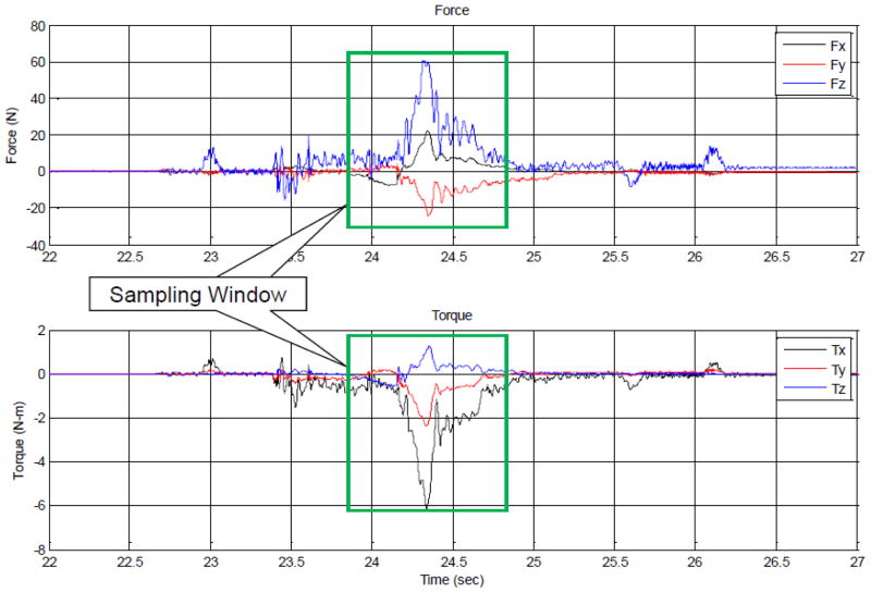
Each failure class has different forces and duration time of the crashing between capillaries or the capillary and the gripper. This information is helpful to label manipulation failures and take corresponding recovery actions. Figure 5 shows typical sampled force/torque data knowing the first failure class. Obviously, F_z and T_x show the most significant changes when manipulation failures happen because the service robot moves vertically while picking up a capillary, and bent tubes cause torques around a horizontal axis. The duration time is around one second, which is used as the sampling window.

Figure 5.

Sampled raw force/torque data from the force/torque sensor in the Cartesian coordinates (force: F_x, F_y, F_z; torque: T_x, T_y, T_z).

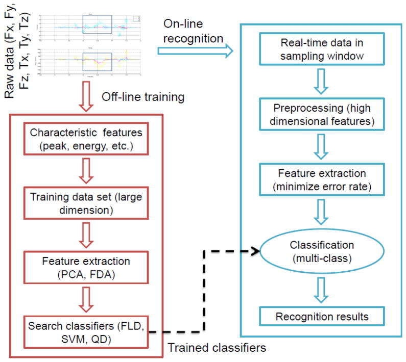
Figure 6 illustrates the procedure of failure recognition. The offline classifier training is to search for optimized classifiers for a given training data set (force/torque data of repeated experimental failures). The online fault recognition is to make a classification decision with the trained classifiers when manipulation failures happen in the RABiT. All of raw sampling data are passed through a low-pass filter to reduce noises. Characteristic features, such as peak value, duration time, and signal energy, are calculated for the following recognition steps.

Figure 6.

Recognition procedure of robotic manipulation failures.

After the failure diagnosis, different recovery schemes are employed. When the class 1 failure occurs, the RABiT must stop the movement of the robot immediately, and send an emergency alert to the operator. Then the operator manually removes the undisposed capillary, and restarts the robot. As to the class 2 failure, automated recovery is implemented because the current capillary is not destroyed. The RABiT identifies the arm length (ratio of torque and force) and then calculate the corresponding position offset in 3D Cartesian coordinates to negate the arm length. The service robot will adjust the picking position of the desired new capillary accordingly and try to pick it up again. As to the failure of class 3, a semi-automated recovery is implemented. Although the current capillary is destroyed, the position offset can be known through the automated analysis of force/torque information. A logical and efficient sequence is to pass over this bent capillary, move onto next one with a position adjustment to account for the large misalignment.

4. Methods of Failure Recognition

Recognition algorithms for feature extraction and classification are briefly summarized below for the self-containment of the paper.

4.1 Feature Extraction

Two linear methods of feature extraction: PCA and FDA, are employed to reduce the dimension of a characteristic feature space. The critical evaluation criterion is the separability of the resultant classes.

The feature extraction is identical to an optimization problem that given a training data set, find the best linear transformation function:

$$z=W^{T}x+b$$ (1)

where original feature vector x ∈ Rⁿ, extracted feature vector z ∈ R^m, transformation matrix W ∈ R^n×m, and the threshold b ∈ R^m After transformation, the corresponding scatter matrices are [11]:

$$S_w^{\ast }=W^T{S}_{w}W,S_b^{\ast }=W^T{S}_{b}W,S_t^{\ast }=W^T{S}_{t}W$$ (2)

where S_w is within-class scatter matrix, S_b is between-class scatter matrix and S_t is total-class scatter matrix.

PCA considers the following reconstruction model for feature vector x̃ ∈ Rⁿ as:

$$\stackrel{\sim }{x}=W(z-b)=\stackrel{\sim }{b}+\sum _{i=1}^m{z}_i{w}_i$$ (3)

where vector b̃ = −W_b ∈ Rⁿ, w_i is the i^th column of W, and z_i is the element of the extracted feature vector. Then minimizing the criterion function:

$$J(W)=\sum _{k=1}^l{\Vert \left(\stackrel{\sim }{b}+\sum _{i=1}^m{z}_{ki}{w}_i\right)-x_k\Vert }^2$$ (4)

is to find matrix $W=[\begin{array}{cccc}{w}_1& w_2& \cdots & w_m\end{array}]$ where l is the number of data points. This can be formulated as the following constrained optimization problem:

$$\begin{array}{l}max{J}_{\mathit{PCA}}(W)=\mid W^T{S}_{t}W\mid \\ \mathit{subject}to{w}_i^T{w}_i=1\end{array}$$ (5)

where w_i is the i^th normalized eigenvector of the scatter matrix S_t corresponding to the ith eigenvalue.

If the sample class labels were known, FDA is able to be used for the supervised dimension reduction. FDA seeks the transformation function (Equation 1) that maximizes the ratio of the between-class scatter matrix to the within-class scatter matrix and the problem is defined as:

$$\begin{array}{l}max{J}_{\mathit{FDA}}(W)=\frac{\mid W^T{S}_{b}W\mid }{\mid W^T{S}_{w}W\mid }\\ \mathit{subject}to{w}_i^T{w}_i=1\end{array}$$ (6)

The solution matrix W = [w₁, w₂, … w_m] is composed by a set of generalized eigenvectors corresponding to the m largest eigenvalues {λ₁, λ₂, … λ_m} in S_bw_i = λ_iS_ww_i [12]. When S_w is nonsingular it can be solved by a conventional eigenvalue problem by $S_w^{-1}{S}_b{w}_i={\lambda }_i{w}_i$. For many small size problem, $S_w^{-1}$ does not exist and has an upper bound m ≤ c − 1 (c is the number of classes) [13].

4.2 Classification Algorithm

The aim of the SVM classifier is to maximize the margin between classes as a way to distinguish them [8]. Under the case of linear separability, the decision rule g(x) = w^Tx + b can be constructed by solving the optimization problem as:

$$\begin{array}{l}max{J}_{\mathit{SVM}}(w)=\frac{1}{2}{\left|\right|w\left|\right|}^2\\ \mathit{subject}to{y}_i(w^{T}x+b)\ge 1,i=1,2,\dots l\end{array}$$ (7)

where y_i is labeled as +1 or −1. Then for the two-class problem, SVM has a margin of $\frac{2}{\left|\right|w\left|\right|}$.

The FLD is a linear discriminant classifier g(x) = w^Tx + b [14], where w is to maximize the class separability. The optimization problem is formulated as:

$$\begin{array}{l}max{J}_{\mathit{FLD}}(W)=\frac{\mid w^T{S}_{b}w\mid }{\mid w^T{S}_{w}w\mid }\\ \mathit{subject}to{w}^{T}w=1\end{array}$$ (8)

This can be observed as a generalized Rayleigh quotient, and thus, for two-class problem, assuming S_w is nonsingular, it is possible to find an analytics expression w = S_w⁻¹ (μ₁ − μ₂), where μ₁, μ₂ are the mean values of two classes. Threshold b is determined by “Bayesian decision theory” or any general classifier.

Different from linear classifiers, the decision rule of the QDA classifier is a quadratic function like g(x) = x^TQx + W^Tx + b [15]. The resultant nonlinear classification hyperplane is able to compass more data points than the linear hyperplane such that the classification error rate is supposed to be lower.

4.3 Classification Error Rate Analysis

To derive an analytic classification error function for a parametric recognition problem, all feature data are assumed to be normally distributed. Based on the extracted feature vectors of the training data, mean values (expected values), and standard deviations are known. Thus the Gaussian probability density functions of three failure classes (ω₁, ω₂, ω₃) are derived as:

$$f_i(x)=\frac{1}{{(2\pi )}^{\frac{n}{2}}{\mid {\mathrm{\sum }}_i\mid }^{\frac{1}{2}}}\mathit{exp}\left[-\frac{1}{2}{(x-{\mu }_i)}^T{\mathrm{\sum }}_i^{-1}(x-{\mu }_i)\right],i=1,2,3$$ (9)

where Σ_i is the i^th covariance matrix. If all classification decisions are based on the Bayesian decision rule, the classification error probability of a three-class problem is described as:

$$\begin{array}{r}{P}_{\mathit{error}}=\int \cdots {\int }_{D_{12}}{f}_2(x)P({\omega }_2){dx}_1\cdots {dx}_n+\int \cdots {\int }_{D_{13}}{f}_3(x)P({\omega }_3){dx}_1\cdots {dx}_n+\\ \int \cdots {\int }_{D_{21}}{f}_1(x)P({\omega }_1){dx}_1\cdots {dx}_n+\int \cdots {\int }_{D_{23}}{f}_3(x)P({\omega }_3){dx}_1\cdots {dx}_n+\\ \int \cdots {\int }_{D_{31}}{f}_1(x)P({\omega }_1){dx}_1\cdots {dx}_n+\int \cdots {\int }_{D_{32}}{f}_2(x)P({\omega }_2){dx}_1\cdots {dx}_n]\end{array}$$ (10)

where P(ω_i), i = 1,2,3, is the probability of class i, D_ij is the feature area where points which are belong to class j are classified as class i because f_i(x) > f_j(x), i,j = 1,2,3, i ≠ j. Equation 10 can be solved by numerical methods for high dimensional data and multiple classes and used to evaluate the performance of feature extraction (Table 2).

Table 2.

Estimated classification error on the extracted feature plane

Dimension of Original Feature	PCA Error Rate (%)	FDA Error Rate (%)
12	2.5467	0.0056
10	3.0456	0.0850
8	3.1267	1.0154
6	3.2281	2.2281
4	2.8190	2.3349

5. Experimental Conditions

Training data are collected by conducting repeated failure experiments of manipulating capillaries in the cell harvesting module of the RABiT system. Failure classes (Figure 4) are denoted as class 1 (no disposing), class 2 (small misalignment) and class 3 (big misalignment). In class 1, the previous tube is purposely not disposed. In class 2, the center line of the gripper is misaligned to that of the new capillary by half of the diameter of the collet (2.5 mm). While in class 3, the misalignment is 4.1 mm, half of the diameter of the outer tubing of the gripper.

The force/torque sensor is from ATI (9105-GAMMA-R-10-U2-N0, 0.01% full-scale error). The real-time sampling system is based on MATLAB xPC target and an analogy I/O card (ServoToGo, ISA Bus Servo I/O Card Model 2). The sampling rate is 1 KHz and the sampling window is 1.0 sec. Before extracting information from the signals, the raw data from the force sensor is passed through a low-pass filter (cutoff frequency 100 Hz, order 8) to reduce high frequency noise.

The experiments of each failure class are repeated 30 times. Thus the training data set has 90 six-dimensional data vectors. The force/torque data in the form of (F_X, F_Y, F_Z, T_X, T_Y, T_Z) is obtained by multiplying the strain gage data from the sensor by a calibration matrix. The robot is set to run at half speed (1 m/s). To alleviate force/torque noise due to the robot’s rapid moving acceleration and deceleration, the smooth path planning is created with zero initial/end velocities and accelerations.

6. Results and Discussion

6.1 Characteristic Feature Selection

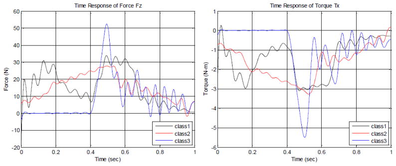
Two most significantly varying signals F_Z and T_X (Section 3, Figure 5) are chosen for failure recognition. The duration time is chosen to be the time when the signal is above $\frac{\sqrt{2}}{2}$ of the max or the signal is below $\frac{\sqrt{2}}{2}$ of the min. It turns out to be around one second as seen in Figure 7.

Figure 7.

Time responses of F_z and T_x of the three failure modes.

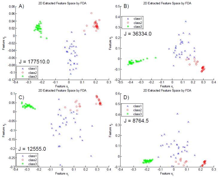
Figure 8 shows the extracted feature planes by an optimal FDA transformation from original high dimensional (twelve-dimensional, eight-dimensional, six-dimensional, four-dimensional respectively) features to two-dimensional (2D) features (x₁, x₂). The 12D space is formed when the max/min value, peak to peak value, mean, standard deviation, energy (curve integration with respect to time), and kurtosis are chosen as the features of F_Z and T_X. The separability index ( $S_b^{\ast }/S_w^{\ast }$) is also indicated in the figure. With decreased dimension of original feature space, the class separability is decreased significantly. For the application presented in the paper, the best class separability for FDA is achieved using the 12D feature.

Figure 8.

Comparison of the feature extraction results of the different original statistical features (A: 12D statistical feature space; B: 8D statistical feature space; C: 6D statistical feature space; D: 4D statistical feature space). Their separability index ( $\mathit{J}={\mathit{S}}_{\mathit{b}}^{\ast }/{\mathit{S}}_{\mathit{w}}^{\ast }$).

The max/min value is the transient pulse force/torque when the capillary gripper collides with the capillary, which reflects the level of distortion of the capillary tubes at the picking position. The peak to peak value also implies the relative magnitude of collision shock. The mean value describes what type of force/torque is involved during the capillary manipulation. For the continuous spring contacting force, the mean value is high, like class 2. While, for the transient collision torque/force (unrecovered elastic force), like class 1 and class 3, the mean value is low. The standard deviation shows how spread-out the torque/force are, a key point to describe the vibration of the signals. The energy implies how long and how much force/torque are engaged on capillaries. Lastly, the kurtosis refers to signal shape and measures to what degree the signal has a flat top or sharp peak profile.

6.2 PCA Versus FDA

PCA seeks principal directions that best represent the original data, while FDA seeks directions that are efficient for separating the data from different classes. Our work is mainly focused on the separability of the failure classes when choosing feature methods for the RABiT system. Therefore, FDA seems to be more appropriate and yet the separability of the resultant low dimensional training data is computed to make comparison between PCA and FDA.

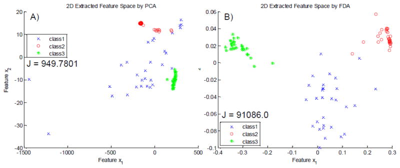
Figure 9 shows the extracted feature planes of the three failure classes by PCA and FDA from the same ten-dimensional features. As seen, the class separability index ( $S_b^{\ast }/S_w^{\ast }$) of FDA is about 96 times higher than that of PCA. For class 1, the extracted feature space by the PCA is undesirable because it almost spreads the whole plane area and especially two points near the bottom left corner are far away from other data points. The PCA is incapable of clustering these two points closer to the center of the group. Another drawback of the PCA is that some points of class 1 are overlapped with those of class 2 and class 3. The overlapped region is likely to lead to large classification error. On the other hand, the FDA is limited in computing the inverse of matrix S_w. If the dimension of feature vectors is high, the matrix S_w is close to be singular and thus it is impossible to be solved directly [16].

Figure 9.

Comparison of the feature extraction methods between PCA (A) and FDA (B). Their separability index ( $\mathit{J}={\mathit{S}}_{\mathit{b}}^{\ast }/{\mathit{S}}_{\mathit{w}}^{\ast }$).

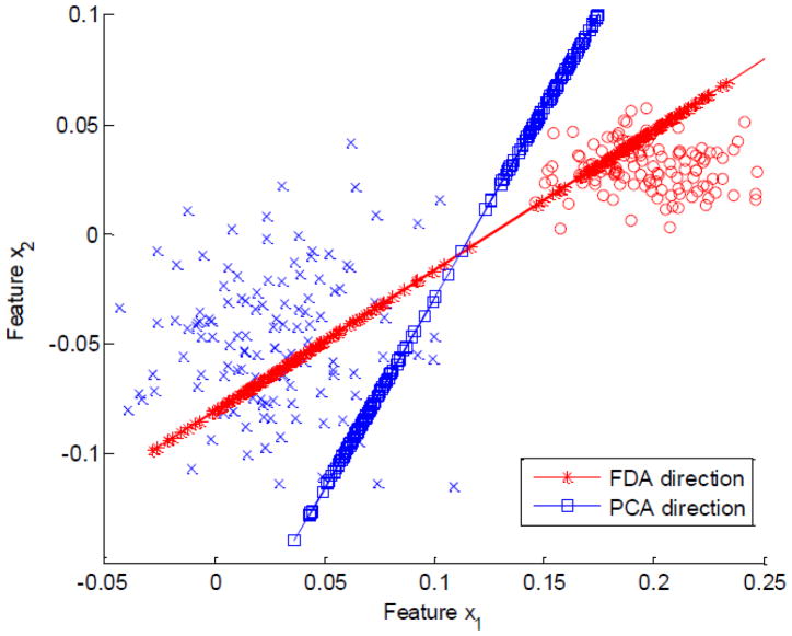
Table 1 presents the separability index after feature extraction by PCA and FDA from 12D feature to 2D feature. The class separability of the FDA increases with the dimensions of original features. Higher dimension of original features allows more space for the FDA to search for the transformation function and thus achieve better performance. For the PCA, although to minimize the feature reconstruction error may be a good criterion, in many cases it does not necessarily lead to maximum class separability in lower dimensional feature spaces. So the separability of the PCA for four dimensions in Table 1 turns out be to larger than that of six dimensions, although its reconstruction error is worse. Figure 10 shows an example of a two-class feature extraction from 2D to 1D where feature vectors in the two classes follow the Gaussian distribution with the same covariance matrix. The eigenvectors of the scatter matrix are computed and the resultant largest eigenvector are visually presented as a PCA projection direction line. Obviously the PCA direction is worse with respect to the separability because the two classes coincide after the features are projected on the PCA direction.

Table 1.

Class separability index after feature extraction

Dimension of Original Feature	PCA	FDA
12	1226.7	177510.0
10	949.7801	91086.0
8	839.2027	36334.0
6	796.8680	12555.0
4	1050.4	8764.5

Figure 10.

PCA is not always best for pattern recognition. Projection on PCA direction makes the two classes coincide. While, projection on FDA direction keeps the classes separated.

Because the main aim of feature extraction problems for the manipulation failure recognition presented in this paper is the separability of the resulting failure classes, FDA achieves better separability index than PCA. The subsequent classifiers are computed based on the training data whose features are extracted by FDA.

6.3 Classification Error Rate

To solve the classification error rate by analytic error probability functions (Equation 8), the following assumptions are made: the probabilities of failures for each failure class are normal distributed; the mean and covariance of the training data are very close to expected values; classification decisions comply with the Bayesian decision rule. For the problem on a 2D extracted feature plane, instead of integrating over an infinite plan, the numerical result of Equation 8 is achieved by integrating over a large enough area (10 times covariance on each side of the mean).

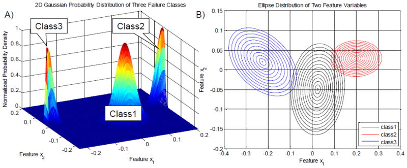
Figure 11 shows normal Gaussian distribution probability density for the extracted features presented in Figure 9B. To solve the analytic classification error probability function, each probability distribution density function is characterized by an ellipse on the feature plane (Figure 11B). The covariance matrices of class 1 and class 2 are close to be diagonal because the major and minor axes of their distribution ellipses (Figure 11B) are nearly parallel to the feature axes each other. Therefore the 2D probability density function of class 1 and class 2 are able to be decoupled into two one-dimensional (1D) probability density functions. Since the major axes of class 3 distribution ellipses are significantly sloped, the off diagonal elements of the covariance matrix of class 3 are non-negligible. Its probability density function has to be coupled two dimensions.

Figure 11.

Gaussian probability distribution of the three failure classes (A: normalized 2D probability density function, B: multivariable distribution ellipses in the 2D feature plane).

Table 2 shows the estimated classification error rate of the three-class problem on the 2D extracted feature plane. Estimated error rate of PCA is bigger than that of FDA. It is consistent with the class separability shown in Table 1. The lower classification error rate for four dimensions for PCA means is an exception and it perhaps means that the derived PCA extraction function (projection direction) happens to improve the class separability, although it minimizes the reconstruction error.

6.4 Classifier Comparison

Three typical classifiers: SVM, FLD, and QDA are tested for the failure recognition of the robotic manipulations in the RABiT. Figure 9B shows that the three failure classes in the extracted feature plane are separated well. Thus simple classification methods are good adequate. In addition, these classifiers incur lower computation costs as their computing time is relatively low, which is helpful for online fault recognition in a high throughput automation system.

Figure 12 shows that the decision boundaries (red and blue lines) and the testing data (three classes, 30 points per class) of three derived classifiers (SVM, FLD and QDA). The testing data is already projected on 2D plan from 12D feature space by a FDA transformation function.

Figure 12.

Classification for the testing data (A: SVM classifier, B: fisher linear classifier, C: quadratic classifier).

Although the classification error rate is calculated based on the analytic probability function (Table 2), the results are limited due to the assumptions made in deriving the analytic probability function (Equation 8). To directly evaluate the classification error for classifiers SVM, FLD and QDA, classification is run on a set of testing data whose class labels are already known. Comparing resultant classified labels with correct class labels, the confusion matrix and the error rate are calculated. As to the testing data shown in Figure 12, the classification error of SVM, FLD, and QDA is 1.1%, 4.4%, and 0.0%, respectively. Because the derived quadratic classifier follows up the distribution shape, such as ellipses in Figure 11B, it leads to the lowest classification error. SVM searches for the classifier while concerning about the small distance space between the classifier and nearest data point. This tolerant space allows the classifier to cover more points if some testing points go further away from the nearest data point of the training data. Therefore, the classification error of SVM lies between QDA and FLD.

6.5 Computation Time

In a high throughput system, like the RABiT, the computation time is a valuable criterion to evaluate the performance of the classifiers because the short interval between each processing action requires a rapid recognition response including logging sensor data, extracting features and making decision. In the RABiT, the service robot moves with a maximum speed 2 m/s. The interval time between the end of picking up a capillary and laser cutting is only 0.45 sec within which the failure diagnosis engine must finish the online processing (Figure 6). For rapid response when failures occur, it is critical to shut down the laser beam immediately before the operator could go in the system to rescue blood samples. Since the computation is programmed in MATLAB, a relative comparison of computation cost is needed among different classifiers and feature extraction methods.

The total computation time is the sum of the time consumption of feature extraction and classification. The feature extraction and classification problems discussed above are in 2D spaces. Obviously the corresponding 1D problem should have less computation but worse performance because of distortions occured during processing data. Table 3 shows the relative comparison of computation time between 2D and 1D problems. The computation difference between the 2D problem and the 1D problem is less than 0.015 sec, which is not worth to switch from 2D to 1D. As to feature extraction, the computation cost of PCA is 10.3 percent larger than that of FLD. It supports the conclusion that FDA is better than PCA for the feature extraction of the force/torque signals in the RABiT (Section 6.2). While as to classification methods, the computation cost of QDA is 90.5 percent larger than that of SVM, although QDA has smaller classification error. It is a trade-off between classification error and response time while choosing SVM or QDA as the classifier.

Table 3.

Computation time cost

	2D (sec)	1D (sec)
FDA	0.0680	0.0618
PCA	0.0750	0.0722
SVM	0.0698	0.0642
FLD	0.1216	0.1136
Quadratic	0.1330	0.1303

7. Conclusions

The proposed automated diagnosis scheme aims to detect and isolate three faults in the cell harvesting, from which three remedial actions: manual recovery, fully automated recovery, and semi-automated recovery, can be taken. The Force on Z axis (F_z) and the torque on X axis (T_x) are the most significant varying signals when the failures happen. Their max/min value, peak to peak value, mean, standard deviation, energy, and kurtosis are calculated from raw sampled data to construct a 12D feature space. The feature transformation functions of PCA and FDA are derived by solving optimization problems as to the failure training data set (three classes, 30 points per class). FDA has the better separability performance and minimal estimated classification error than those of PCA when projecting 12D feature space to 2D feature plane. While PCA spends 10.3% more computing time than FDA.

Three classifiers: SVM, FLD and QDA are implemented and compared. They are solved offline based on the training data set. Their online fault diagnosis performances are evaluated through the testing data set (three classes, 30 points per class). QDA incurs the minimal classification error, while SVM takes the minimal computation time. Considering the tradeoff between classification error and response time, the SVM is chosen for fault recognition under the current configuration of the RABiT.

References

- 1.Pellmar TC, Rockwell S. Priority List of Research Areas for Radiological Nuclear Threat Countermeasures. Radiation Research. 2009;163(1):115–123. doi: 10.1667/rr3283. [DOI] [PubMed] [Google Scholar]
- 2.Chen Y, et al. Development of a Robotically-based Automated Biodosimetry Tool for High-throughput Radiological Triage. International Journal of Biomechatronics and Biomedical Robotics. 2010;1(2):115–125. [Google Scholar]
- 3.Chandrababu S, Christensen HI. Adding diagnostics to intelligent robot systems. Intelligent Robots and Systems; 2009; IROS 2009. IEEE/RSJ International Conference on; 2009. [Google Scholar]
- 4.Venkatasubramanian V, et al. A review of process fault detection and diagnosis Part III: Process history based methods. Computers & Chemical Engineering. 2003;27(3):327–346. [Google Scholar]
- 5.Cho HW. Identification of contributing variables using kernel-based discriminant modeling and reconstruction. Expert Systems with Applications. 2007;33(2):274–285. [Google Scholar]
- 6.Akbaryan F, Bishnoi PR. Fault diagnosis of multivariate systems using pattern recognition and multisensor data analysis technique. Computers & Chemical Engineering. 2001;25(9–10):1313–1339. [Google Scholar]
- 7.Theodoridis S, Koutroumbas K. Pattern recognition. 3. xvi. Amsterdam ; Boston: Elsevier/Academic Press; 2006. p. 837. [Google Scholar]
- 8.Burges CJC. A tutorial on Support Vector Machines for pattern recognition. Data Mining and Knowledge Discovery. 1998;2(2):121–167. [Google Scholar]
- 9.Chapelle O, et al. Choosing multiple parameters for support vector machines. Machine Learning. 2002;46(1–3):131–159. [Google Scholar]
- 10.Bredensteiner EJ, Bennett KP. Multicategory classification by support vector machines. Computational Optimization and Applications. 1999;12(1–3):53–79. [Google Scholar]
- 11.Duda RO, Hart PE, Stork DG. Pattern classification. 2. xx. New York: Wiley; 2001. p. 654. [Google Scholar]
- 12.Belhumeur PN, Hespanha JP, Kriegman DJ. Eigenfaces vs. Fisherfaces: recognition using class specific linear projection. Pattern Analysis and Machine Intelligence, IEEE Transactions on. 1997;19(7):711–720. [Google Scholar]
- 13.Martinez AM, Kak AC. PCA versus LDA. Pattern Analysis and Machine Intelligence, IEEE Transactions on. 2001;23(2):228–233. [Google Scholar]
- 14.Fukunaga K. Computer science and scientific computing. Academic Press; Boston: 1990. Introduction to statistical pattern recognition. [Google Scholar]
- 15.WAKAKI H. Comparison of linear and quadratic discriminant functions. Biometrika. 1990;77(1):227–229. [Google Scholar]
- 16.Mika S, et al. Fisher discriminant analysis with kernels. Neural Networks for Signal Processing IX; 1999; Proceedings of the 1999 IEEE Signal Processing Society Workshop; 1999. [Google Scholar]