Live-Cell Fluorescence Microscopy with Molecular Biosensors: What Are We Really Measuring?

Abstract

Engineered protein biosensors, such as those based on Förster resonance energy transfer, membrane translocation, or solvatochromic shift, are being used in combination with live-cell fluorescence microscopy to reveal kinetics and spatial localization of intracellular processes as they occur. Progress in the application of this approach has been steady, yet its general suitability for quantitative measurements remains unclear. To address the pitfalls of the biosensor approach in quantitative terms, simple reaction-diffusion models were analyzed. The analysis shows that although high-affinity molecular recognition allows robust detection of the fluorescence readout, either of two detrimental effects is fostered. Binding of an intramolecular biosensor or of a relatively abundant intermolecular biosensor introduces observer effects in which the dynamics of the target molecule under study are significantly perturbed, whereas binding of a sparingly expressed intermolecular biosensor is subject to a saturation effect, where the pool of unbound biosensor is significantly depleted. The analysis explores how these effects are manifest in the kinetics and spatial gradients of the biosensor-target complex. A sobering insight emerges: the observer or saturation effect is always significant; the question is whether or not it can be tolerated or accounted for. The challenge in managing the adverse effects is that specification of the biosensor-target affinity to within a certain order of magnitude is required.

Introduction

If our mechanistic understanding of cell regulation is to dramatically advance, existing methods for quantifying concentrations and activity states of intracellular molecules will need to be improved, and new ones will need to be developed. Although biochemical assays are commonly used and can be quantitative if performed carefully, these methods offer no direct information about cell-to-cell heterogeneity or subcellular localization. Other methods, such as flow cytometry and immunofluorescence, address one or both of these issues but are nonetheless end-point assays with respect to kinetics. In contrast, live-cell microscopy uniquely elucidates spatiotemporal dynamics of intracellular processes in real-time and at the single-cell level, i.e., in conjunction with observations of cell behavior (1–4).

Two distinct variations of this method have been used extensively:

In the first, a full-length protein or other molecule found in the cell is tagged with a fluorescent protein or dye, and the subcellular localization of the conjugate is monitored by various modes of fluorescence microscopy (5). We may refer to this as the “biomarker approach”. This approach has been successfully (and cleverly) applied to elucidate quantitative aspects of cytoskeletal and focal adhesion dynamics (for example, Danuser and Waterman-Storer (6) and Kolin and Wiseman (7)); however, it has certain limitations. Biomarkers indicate dynamic localization of the tagged molecule but not changes in its activity or modification states. Moreover, the subcellular localization of a protein is often affected by multiple factors (protein-protein and protein-lipid interactions and posttranslational modifications), in which case the measurement is challenging to interpret from a molecular standpoint.

The second variation strives to overcome those limitations through the introduction of an engineered fluorescent probe or protein construct that possesses minimal molecular recognition. We refer to this as the “biosensor approach”. By engaging in a specific binding interaction to form a noncovalent complex, the biosensor yields a fluorescence readout that is meant to indicate the state or abundance of a particular target. In early applications of the biosensor approach, fluorescent probes were developed to measure intracellular concentrations of small molecules, most notably calcium and cAMP. Protein domains and motifs have since been used to distinguish between activity or modification states of protein and lipid targets (8). Irrespective of the molecular details, intracellular biosensors may be classified as either intramolecular, where the molecular recognition element and its target are contained within the same chain (connected by a flexible linker), or intermolecular, where the recognition module binds to form a bimolecular complex with a target that is endogenous to the cell (Fig. 1) (9,10). Biosensors of the first type include those based on intramolecular Förster resonance energy transfer, with donor and acceptor fluorophores flanking the two ends of the chain; this approach has been applied most prominently to study signaling mediated by small GTPases (11–14) and protein kinases (15–20). Intermolecular biosensors include those based on membrane translocation (21–26) or solvent-sensitive fluorescence (27,28).

Figure 1.

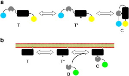
Two general classes of molecular biosensors. (a) An intramolecular biosensor contains both the target and molecular recognition element, connected by a linker. The inactive target T is activated by an endogenous intracellular process to produce the active, unoccupied target T^∗; the activated state is bound by the molecular recognition element to form the complex C, generating the biosensor readout. (Illustration) Common scenario where intramolecular binding brings a Förster resonance energy transfer pair into close proximity. (b) An intermolecular biosensor, B, contains a molecular recognition element that binds to an endogenous target to form a bimolecular complex, C. (Illustration) Common scenario where complex formation results in membrane translocation of the tagged biosensor.

The biosensor approach is not without its own limitations. As of this writing, there are only a small number of validated biosensors, as compared with the broad palette of antibodies available. More critically, the biosensor readout cannot perfectly report the intracellular process being studied. The ideal condition may be stated thus: the biosensor-based measurement ought to be proportional to the target concentration (at any given time and intracellular location) that would have been present if molecular recognition by the biosensor did not occur. To the uninitiated observer, this might seem to be a reasonable assumption; however, it presents a clear paradox. Without molecular recognition, there is no signal, but formation of the complex masks the active target from deactivating enzymes and endogenous effectors. This issue, an example of the observer effect in physics, is endemic to the biosensor approach.

Although the general nature of the problem is intuitive and has been recognized for some time (29,30), the following questions have not been addressed in detail:

• First, in what specific ways does the biosensor readout deviate from the ideal response?

• Second, for each of those, how does the severity of the problem depend on the properties of the biosensor and of the system under study?

• Finally, how and to what extent might those issues be avoided while also allowing for a reliably detectable signal?

Answers are provided here through the analysis of simple reaction-diffusion models.

Materials and Methods

Model equations

It is supposed that the fluorescence readout is directly related to the local concentration (or, in the case of a membrane-associated species, the area density) of a biosensor complex, C. The key assumption is that the complex is sequestered and thus shielded from participating in other reactions. Thus, the conservation of the complex is governed by net diffusion (advective or motor-driven transport could be added if warranted) and binding as follows:

$$\frac{\partial C}{\partial t}=D_C{\nabla }^{2}C+v_{bind}.$$ (1)

The rate term v_bind accounts for reversible binding, and two scenarios are considered: intramolecular and intermolecular binding (Fig. 1). In the intramolecular case, the target species is fused with the biosensor, and once activated, the biosensor transitions reversibly between activated and unbound (T^∗) and bound (C) forms. In the intermolecular case, the T^∗ species forms a complex with a fluorescent biosensor (local concentration [B]) to form C. According to mass action,

$$v_{bind}=\{\begin{array}{l}{k}_{on}{T}^{\ast }-k_{off}C,\text{intramolecular};\\ k_{on}\left[B\right]T^{\ast }-k_{off}C,\text{intermolecular}.\end{array}$$ (2)

In both cases, the free target becomes available via an activation process, T → T^∗, with local rate v_act. Activation is reversed via deactivation with local rate v_deact. A more complete model would additionally account for target interactions with endogenous binding partners. With the common assumption of slow synthesis and turnover rates, the balances for the inactive and active target forms are as follows:

$$\frac{\partial T}{\partial t}=D_T{\nabla }^{2}T-v_{act}+v_{deact},$$ (3)

$$\frac{\partial T^{\ast }}{\partial t}=D_{T^{\ast }}{\nabla }^2{T}^{\ast }+v_{act}-v_{deact}-v_{bind}.$$ (4)

The simplest plausible rate laws for v_act and v_deact were assumed as follows:

$$v_{act}=k_{act}S\left(t,x\right)T,$$ (5)

$$v_{deact}=k_{deact}{T}^{\ast }.$$ (6)

Thus, the temporal or spatial dependence of the response is driven by a case-specific signal function, S(t,x).

In the intermolecular case, the conservation of the free biosensor must also be accounted for, and in so doing one would need to consider whether complex formation occurs in the same cellular compartment or involves translocation of the biosensor from the cytosol to a membrane surface (m). The latter is assumed to be the case here; further assuming slow synthesis and turnover of the biosensor,

$$\frac{\partial \left[B\right]}{\partial t}=D_B{\nabla }^2\left[B\right];D_B{\left(\mathbf{n}·\nabla \left[B\right]\right)|}_m={v_{bind}|}_m.$$ (7)

Note that in Eq. 7 and in Eq. 8 below, conversion between numbers of molecules and moles as needed is implicit.

For analysis, models are often simplified by assuming well-mixed compartments (as in Figs. 2–4). In that case, the diffusion terms in Eqs. 1, 3, and 4 are neglected, and Eq. 7 reduces to

$$\begin{array}{c}\frac{d\left[B\right]}{dt}=-\frac{A_{mem}}{V_{cyt}}{v}_{bind},\\ \left[B\right]\left(t\right)={\left[B\right]}_0-\frac{A_{mem}}{V_{cyt}}C\left(t\right),\end{array}$$ (8)

where A_mem/V_cyt is the ratio of the membrane surface area divided by the volume of cytosol, and [B]₀ is the free biosensor concentration when no active target is present.

Figure 2.

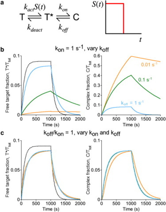
Perturbation of active target level and kinetics: intramolecular biosensors, or intermolecular biosensors expressed in stoichiometric excess. (a) Kinetic scheme for an intramolecular biosensor, following the nomenclature established in Fig. 1a; the scheme holds equally for an intermolecular biosensor expressed in excess ([B] ≈ constant). In the hypothetical scenario, stimulation (S = 1) is pulsed for a period of 1000 s. (b) The fractions of the total biosensor pool in the free, active target (T^∗, left) and complexed (C, right) states are plotted as a function of time. The affinity of the molecular recognition element was adjusted by progressively decreasing the dissociation rate constant k_off, as indicated: k_off = 1 s⁻¹, 0.1 s⁻¹, or 0.01 s⁻¹. (Dashed curve) Active target kinetics in the absence of complex formation (k_off = ∞). Other parameter values were fixed at k_on = 1 s⁻¹, k_act = 0.001 s⁻¹, and k_deact = 0.01 s⁻¹. (c) Same as panel b, except that the ratio of k_off/k_on was fixed at 1, with k_off = k_on = 1 s⁻¹, 0.1 s⁻¹, or 0.01 s⁻¹.

Figure 3.

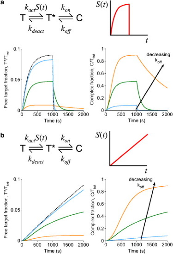
Response of an intramolecular biosensor to gradually changing input. (a) Assuming the kinetic scheme depicted for an intramolecular biosensor, the scenario presented in Fig. 2 was altered so that the activation of the target during the first 1000 s is more gradual, with S(t) = 1 – exp(−0.005t) (t in s). The fractions of the total biosensor pool in the free, active target (T^∗, left) and complexed (C, right) states are plotted as a function of time. The affinity of the biosensor was adjusted by progressively decreasing the dissociation rate constant k_off: k_off = 1 s⁻¹, 0.1 s⁻¹, or 0.01 s⁻¹. Other parameter values were fixed at k_on = 1 s⁻¹, k_act = 0.01 s⁻¹, and k_deact = 0.1 s⁻¹. (b) Same as panel a, except that the stimulation was assumed to follow a linear ramp, with S(t) reaching a value of 1 at t = 2000 s.

Figure 4.

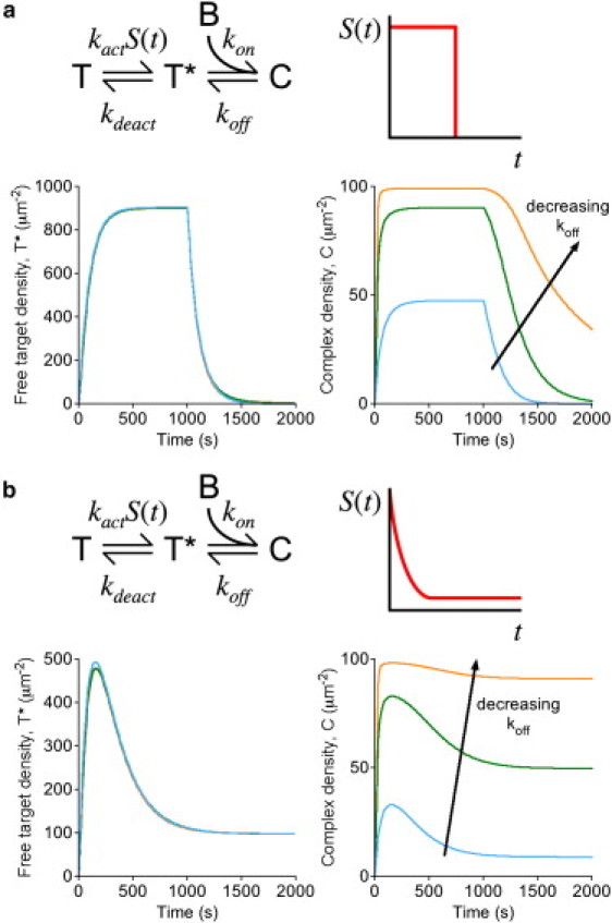
Saturation of the biosensor readout: intermolecular biosensors with active target in excess. (a) Assuming the kinetic scheme depicted for an intermolecular biosensor, applying the nomenclature established in Fig. 1b, stimulation (S = 1) is pulsed for a period of 1000 s. The membrane densities of the free, active target (T^∗, left) and target-biosensor complexes (C, right) are plotted as a function of time. The affinity of the biosensor was adjusted by progressively decreasing the dissociation rate constant k_off: k_off = 1 s⁻¹, 0.1 s⁻¹, or 0.01 s⁻¹. Other parameter values were fixed at T(0) = 10⁴μm⁻², [B]₀ = 0.1 μM, k_on = 1 μM⁻¹ s⁻¹, k_act = 0.001 s⁻¹, and k_deact = 0.01 s⁻¹. (b) Same as panel a, except that the stimulation was assumed to follow incomplete adaptation according to $S\left(t\right)=0.1+0.9\exp \left(-0.005t\right)$ (t in s).

Model implementation

Models were implemented in the Virtual Cell software environment (www.vcell.org) (31) and are publicly accessible under the BioModel “Biosensor simple”. For all models, values of the rate constants are specified in the corresponding figure caption. In Figs. 2, 4, and 5, the value of k_deact was set at 0.01 s⁻¹, consistent with a signaling state lifetime of ∼1 min (e.g., Schneider and Haugh (32)). In Fig. 3, a 10-fold higher value (k_deact = 0.1 s⁻¹) was considered.

Figure 5.

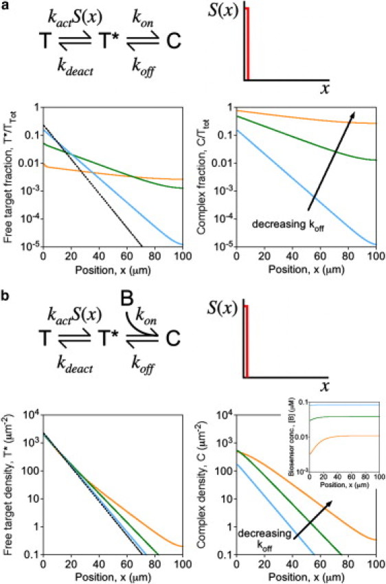
Actual or apparent blurring of spatial gradients. Stimulation is focused in a small region at one end of the cell, and concentration profiles were calculated at steady state. To aid in the evaluation of relative gradient steepness, all concentration profiles are presented as semilog plots. (a) Assuming the kinetic scheme depicted for an intramolecular biosensor, the steady-state fractions of the total biosensor pool in the free, active target (T^∗, left) and complexed (C, right) states are plotted as a function of position. The affinity of the molecular recognition element was adjusted by progressively decreasing the dissociation rate constant k_off: k_off = 1 s⁻¹, 0.1 s⁻¹, or 0.01 s⁻¹. (Dashed curve) Active target kinetics in the absence of complex formation (k_off = ∞). Other parameter values were fixed at k_on = 1 s⁻¹ and k_deact = 0.01 s⁻¹. (b) Same as panel a, except that the kinetic scheme depicted for an intermolecular biosensor was assumed, with T(x,0) = 10⁴μm⁻², [B]₀ = 0.1 μM, and k_on = 1 μM⁻¹ s⁻¹. (Inset) Associated concentration profiles of the free biosensor, [B](x).

For well-mixed compartmental models (Figs. 2–4), the cytosol was assigned a reasonable volume of 1.667 pL = 1667 μm³, such that a concentration of 1 μM corresponds to 10⁶ molecules in that volume; the plasma membrane was assigned an area of 1000 μm².

In models accounting for spatial gradients (Fig. 5), the spatial domain is a thin rectangle with length L = 100 μm (typical length scale for a fully spread and polarized fibroblast) and height = 3.4 μm (to approximately match the A_mem/V_cyt ratio assumed in the compartmental model calculations). A spatially focused stimulus is applied, confined to the small domain x ∈ (0,0.01L); under these conditions, the problem is effectively one-dimensional with a point source at one end. Typical effective diffusivity values were assigned, with D_B = 30 μm²/s for the biosensor in the cytosol and D_T = D_T∗ = D_C = 0.5 μm²/s for all membrane species. For numerical implementation, grid spacings of 0.05 and 0.1 μm were used, yielding approximately identical results.

Results and Discussion

Biosensor binding generally reduces the availability of the active target and slows down its kinetics of accumulation and clearance

We consider the common situation where the active target molecule of interest is not subject to deactivation while it is sequestered in the biosensor complex. For example, at least by all contemporary accounts, recognition of phosphorylated molecules precludes access by phosphatases (33), and binding of effectors to active small GTPases hinders GTP hydrolysis (34–36). To illustrate how this impacts the biosensor output, a simple yet reasonable model of target activation and deactivation is imposed (Fig. 2 a): a step pulse of an external signal turns activation on and off, and the rates of activation and deactivation are linear with respect to substrate concentrations. For now, the model is further simplified by supposing that complex formation is intramolecular. As shown in Fig. 2 b, progressively increasing the affinity of the biosensor complex results in: 1), reduction of the free target concentration at steady state, and 2), increasingly sluggish kinetics relative to the scenario where the complex does not form. The extent of the former effect depends on the extent of activation in the absence of biosensor binding. Thus, for the scenario where as much as half of the active form is in the biosensor complex (C = T^∗), but most target molecules remain inactive at steady state (T = 10T^∗; Fig. 2 b, cyan curves), the steady-state value of T^∗ is reduced by only a modest percentage. By comparison, the effect on kinetics is more direct; if half of the active form is sequestered (k_on = k_off), for example, then the characteristic time to reach steady state is prolonged by roughly a factor of two. As shown in Fig. 2 c (orange curves), additional sluggishness of the biosensor readout begins to appear if the timescales of biosensor complex association and dissociation are not significantly faster than that of target deactivation.

The more intuitive of these effects is the tendency of complex formation to buffer the active target concentration at steady state. The less appreciated but more consistently detrimental effect as shown by the calculations concerns the transient kinetics, as during the response of the system to external stimulation. When the concentration of free target is increasing, the net formation of the complex reduces the rate of free target accumulation (that is, makes it less positive). Conversely, when the concentration of free target is decreasing, the net dissociation of the complex slows the rate of decline (makes it less negative). Thus, complex formation generally causes the system to respond more sluggishly. The adequacy of a biosensor hinges, in part, on the mildness or severity of these effects under various conditions.

The calculations described above effectively assume instantaneous on- and off-states for the upstream signal, S(t). This scenario approximates rapid, receptor-mediated activation followed by rapid, pharmacological inhibition, as considered previously (32,37). In many other situations, the dynamics of S(t) might be relatively slow on the timescale of the mean lifetime of T^∗, 1/k_deact, in which case the ideal biosensor would faithfully track the kinetics of S(t). To evaluate this situation, an alternate scenario in which S(t) increases and approaches a plateau gradually, followed by rapid inhibition of S, was considered (Fig. 3 a). To ensure that the biosensor could more readily respond to changes in S(t), higher values of k_act and k_deact were used here. Although the biosensor response, C(t), is predicted to be robust and roughly matches the timescale of S(t), the decay of the system after rapid inhibition is slowed dramatically for k_on/k_off >> 1 (Fig. 3 a). This disparity between the kinetics of the stimulation and inhibition phases of the hypothetical experiment is consistent with measured kinetics of the c-Jun N-terminal kinase activation reporter (20).

Whereas the C(t) kinetics in the stimulation phase qualitatively reflect those of S(t), quantitative correspondence between the two was found to suffer when k_on/k_off >> 1. To show this definitively, a different scenario was considered in which S(t) increases as a slow, linear ramp (Fig. 3 b). As expected, the biosensor response C(t) deviates perceptibly from linearity for high k_on/k_off. Analysis of the system shows that two effects influence the fidelity of the biosensor response. At short times, the rate of biosensor response is affected according to how severely complex formation prolongs the mean lifetime of the active target, which is approximately equal to (1 + k_on/k_off)/k_deact. At long times, fidelity is limited by the availability of the unbound target when most of the biosensor is driven into the bound state.

From a mathematical point of view, these analyses of intramolecular complex formation hold equally for intermolecular complex formation with the biosensor in vast excess (with k_on replaced by k_on[B], where the free biosensor concentration [B] is approximately constant); however, from a biological point of view, it is important to distinguish the two. In the case of an intramolecular biosensor, the active target is a part of the biosensor itself. Therefore, high-affinity complex formation does not have a direct impact on the endogenous biology (although indirect effects via sequestration of activating/deactivating enzymes and endogenous effectors, beyond the analysis presented here, should be considered). By comparison, an intermolecular biosensor expressed at excessive levels has a buffering effect that not only affects the kinetics of the biosensor readout; more critically, it can act as a dominant negative in terms of biological function.

Suggestive of such a buffering condition, Yip et al. (39) reported that a carcinoma cell line with heterologously expressed Btk pleckstrin homology (PH) domain, which binds to the plasma membrane lipid PtdIns(3,4,5)P₃ with high affinity (K_D = 80 nM (38)), showed a dramatic increase in the half-life of PtdIns(3,4,5)P₃ under otherwise rapid turnover conditions (39). Tagged Btk PH domain has been employed as an intermolecular biosensor because of its unique specificity for PtdIns(3,4,5)P₃ relative to PtdIns(3,4)P₂ (30); however, because of its high affinity, the Btk PH domain can be expected to perturb free PtdIns(3,4,5)P₃ levels and kinetics when expressed at excessive levels in cells.

With intermolecular binding, excess biosensor can affect free target kinetics, whereas excess target can result in a saturated readout

In the previous section, we considered situations in which the fluorescent biosensor is not stoichiometrically limiting for complex formation. The opposite situation, which is relevant only to intermolecular binding, arises when the target molecule is in vast excess and the biosensor affinity is sufficiently high (K_D sufficiently low), such that nearly all of the biosensor molecules in the cell are in complex. This scenario is illustrated for two simple models of target activation: 1), a transient pulse (as in Fig. 2), and 2), a decay with incomplete adaptation. Both sets of associated calculations show that as the active target progressively depletes the limiting pool of available biosensor, the free target is not significantly perturbed; however, the biosensor readout does not quantitatively reflect the free target kinetics. The pulsed activation case (Fig. 4 a) illustrates that the increase in complex formation after stimulation approaches steady state faster than does the free target, because the concentration of available biosensor is initially much higher than its steady-state value. Conversely, after activation is turned off, the decay of the complex is relatively sluggish, as the liberation of free biosensor counterbalances the decay of free target concentration. The incomplete adaptation case (Fig. 4 b) further illustrates that the change in the abundance of the complex (the apparent degree of adaptation) tends to be more modest than the actual change in free target concentration. In the limit of near-complete depletion of available biosensor (Fig. 4 b, orange curves), the adaptation kinetics of the target would be missed completely.

These calculations demonstrate that, when an intermolecular biosensor is limiting for complex formation, perturbation of the free target accumulation or clearance kinetics is minimal. Rather, the issue is that formation of the complex is saturated and thus serves as a poor quantitative readout. A prominent example of the saturation effect is the binding of tagged PLCδ PH domain, which binds the plasma membrane lipid PtdIns(4,5)P₂. In many cells at least, PtdIns(4,5)P₂ is quite abundant; its characteristic concentration on a whole-cell basis has been estimated at 10 μM, which is much higher than the measured biosensor K_D of 2 μM (40). Hence, it is widely appreciated that tagged PLCδ PH tends to be mostly in complex with PtdIns(4,5)P₂ (or with the soluble hydrolysis product, Ins(1,4,5)P₃, in the cytosol) (40), and thus the membrane-localized fluorescence in cells is insensitive to treatments that partially reduce the level of PtdIns(4,5)P₂ by inhibition of its resynthesis (24).

A spatial gradient of free target is made (or appears to be made) less steep as a consequence of biosensor complex formation

The spatial range (or dynamic length scale) of an active chemical species is defined by how far it diffuses on average before reverting to the inactive state. If biosensor-target complexes are not subject to deactivation, it follows from the intuition developed above that the spatial range of the active target would be extended when a significant fraction of it is bound. Thus, formation of the complex makes the active target gradient shallower than it would have been in the absence of binding. This effect has been recognized and discussed in the context of fluorescent biosensors (41), and calculations show that it is relevant to the case of an intramolecular biosensor with high-affinity binding (or an intermolecular biosensor with biosensor in excess) (Fig. 5 a). In the simplified scenario assumed here, a one-dimensional, steady-state gradient is formed via constant activation within a thin strip located at one end of the spatial domain and deactivation throughout. In the absence of complex formation, the concentration profile of the active target is approximately exponential, with a spatial decay constant that scales as the square root of k_deact. Therefore, with an intramolecular biosensor, the steepness of the active target gradient (the negative slope of the gradient on a semilog plot) is affected according to the fraction of the active form that is sequestered. For example, 50% sequestration (C = T^∗) increases the spatial range of the target and thus decreases the steepness of its gradient by a factor of roughly square-root of 2 (Fig. 5 a; compare the cyan and black curves). In more extreme cases, the spatial range is comparable to the cell length, and reflection at the distal boundary tempers the gradient even more (Fig. 5 a, orange curves). Consistent with the analysis presented in Fig. 2 b, the other effect is a reduction in free target concentration at the site of its activation.

The alternative scenario, where the biosensor is intermolecular and the endogenous target is in excess, was also investigated (Fig. 5 b). In this case, based on the analysis presented in Fig. 4, one might predict that biosensor binding would have no appreciable effect on the active target gradient, but the gradient of biosensor-target complexes would not be a faithful reflection thereof. Indeed, the calculations demonstrate that the free target profile is not significantly perturbed (except in the tail of the profile, where the free target concentration is low), while the gradient of bound complex is rendered progressively more shallow as the affinity and lifetime of the biosensor-target complex are enhanced (Fig. 5 b). This effect does not follow directly from the saturation effect illustrated in Fig. 4, however—which is to say that global depletion of the free biosensor does not adequately explain the result. Rather, local depletion of the free biosensor, manifest as an opposing gradient in [B](x), causes the C(x) gradient to be tempered relative to that of T^∗(x) (Fig. 5 b, inset). By manipulating Eqs. 1 and 7 for an effectively one-dimensional system at steady state, it is apparent that

$$V_{cyt}\frac{d\left[B\right]}{dx}=-\frac{D_C}{D_B}\left(A_{mem}\frac{dC}{dx}\right).$$ (9)

Equation 9 shows that, because diffusion in the cytosol is relatively fast (D_B >> D_C), the absolute gradient in the cytosol is always much shallower than that of the membrane-associated complex; however, the relative gradients (fractional changes in [B] and C per unit length) become closer in magnitude with progressively greater binding of the biosensor at that location. Also contributing to the tempering of the observed C(x) gradient is the potential for a long-lived complex (42). This distinct effect is significant when the mean lifetime of the complex (1/k_off) is comparable to or greater than that of the active target (1/k_deact) (Fig. 5 b, orange curves).

Constraints and trade-offs in the practical application of intra- and inter-molecular biosensors for live-cell fluorescence microscopy

The analyses presented above demonstrate the potential pitfalls that might, unbeknownst to the observer, give misleading results in live-cell imaging experiments. Here, reasonably general guidelines are developed for diagnosing and avoiding such issues, framed in terms of the properties of intra- and intermolecular biosensors that might be introduced into cells. Again, the goal of the experimental design is for the concentration of bound complex to accurately reflect changes in activation status of an endogenous target, as they would normally occur. But this ideal must be balanced against the practical consideration of what can be reliably measured by standard fluorescence microscopy.

Let us first consider the properties of an intramolecular biosensor. In this case, the design space is defined by two dimensionless ratios: the k_on/k_off (affinity constant) of intramolecular binding and the context-dependent ratio of target activation and deactivation frequencies in the cell (Fig. 6 a). Through the analyses described in the previous sections, it was demonstrated that if k_on/k_off were too high, the apparent kinetics and spatial pattern of the readout would be perturbed relative to those of the endogenous target (the observer effect). On the other hand, if either the k_on/k_off ratio or the ratio of active/inactive unbound target were too low, there would not be enough of the bound complex C to reliably quantify against the background of fluorescent biosensor molecules in the T and T^∗ states. These competing considerations together define a region of feasibility, wherein one would hope to operate (Fig. 6 a, shaded region). The analysis allows as much as half of the active target to be shielded from deactivation (k_on/k_off ≤ 1) and considers that the readout could be reliably measured if as little as 5% of the biosensor were in the C form. Still, these considerations impose restrictive constraints on both the complex affinity, which must be of intermediate strength, and the extent of target activation, which must be sufficiently high. Obviously, less generous constraints would shrink or altogether eliminate the region of feasibility. Another caveat is that higher values of k_on/k_off could be tolerated, up to a point, when the shape of the temporal or spatial response is not sensitive to the rate of target deactivation, i.e., when the upstream signal S(t,x) changes gradually in time or space (as considered in Fig. 3). Higher k_on/k_off ratios would also be tolerable for biosensors with conformations that breathe enough to allow a nonzero rate of deactivation while in the bound state.

Figure 6.

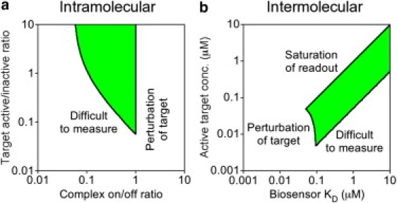
Design space for engineering suitable biosensors. In each case, a desirable region of feasibility is defined by the shaded area. (a) The design space for an intramolecular biosensor is defined by the affinity of complex formation and the extent of target activation. To the left of the desired region, 5% or less of the biosensor molecules are in complex, resulting in a readout that is difficult to measure. To the right of the desired region, 50% or more of the modified target is bound, resulting in significant perturbation of the observed kinetics. (b) The design space for an intermolecular biosensor is defined by the biosensor binding affinity and the concentration of the active target. A moderate biosensor expression level of 0.1 μM is assumed. In addition to the criteria outlined under panel a, saturation of complex formation becomes significant when the active target concentration exceeds both the concentration and binding K_D of the biosensor.

In the case of an intermolecular biosensor, the considerations are similar but with the additional constraint that the readout should not be saturated (complex formation should not be limited by the availability of biosensor). Here, the design space is adequately framed in terms of concentrations: those of the biosensor and active target relative to the value of the intermolecular K_D. The total biosensor concentration is fixed here at [B]₀ = 0.1 μM, because this is at the lower end of fluorescent protein concentrations that are visible by standard fluorescence microscopy; hence, the design space is defined by variable ranges of the active target concentration (calculated on the basis of the cytosolic volume) and K_D (Fig. 6 b). If neither of these values is >0.1 μM, the biosensor concentration is in excess, and the spatiotemporal dynamics of the endogenous target would be significantly perturbed as in the intramolecular case. The other considerations concern the active target concentration in relation to K_D; if it is too low, not enough of the fluorescent biosensor will be in complex, whereas if it is too high, the free biosensor will be significantly depleted, and the measurement will approach saturation. The shaded region of feasibility allows up to 50% depletion of free biosensor and, as before, considers that only 5% of the biosensor needs to be in complex for a reliable measurement (Fig. 6 b). It is concluded that for quantitative studies with an intermolecular biosensor, the active target should be present at a high nanomolar concentration or above, and the ideal biosensor would possess a K_D value moderately above that.

Prospects for truly quantitative live-cell imaging of cell biochemistry

As a cell biology workhorse, live-cell fluorescence microscopy is a powerful approach, and the resulting measurements can be reasonably quantitative if great care is taken. Yet, as illustrated in this article, even perfectly measured live-cell biosensor readouts cannot perfectly track the spatiotemporal dynamics of intracellular processes, and in extreme cases, such measurements can be misleading. Two steps may be taken to mitigate the issue.

First, the binding affinity of a biosensor should be characterized and optimized for a particular application. Practitioners of live-cell microscopy should be aware that high-affinity molecular recognition is not desirable. The traditional approach of using modular-binding domains found in nature is too restrictive in that regard; hence, identifying biosensors using protein-engineering methods (43) presents an attractive alternative. Screening protein variant libraries for desired binding properties is well documented (44).

Second, mathematical models may be used to deconvolute the data so as to account for the deviation from ideality. Provided that the binding affinity and intracellular concentration of the biosensor were known, one could back-calculate the free target concentration or density, T^∗(x,t), from the measured C(x,t). Indeed, mathematical recipes for accomplishing this in the context of calcium imaging have been offered (45), and the use of modeling to account for saturable translocation of phosphoinositide biosensors has been demonstrated previously (32,46). This method is complicated, however, when the target perturbation effect is significant; as illustrated in Fig. 2 b, the free target kinetics might be markedly altered relative to the unperturbed scenario. Fitting the data to a more complete model, including the parameters characterizing endogenous target dynamics, would allow the unperturbed kinetics or spatial pattern to be reconstructed (47), but formulation of such a model requires advance knowledge or strong assumptions about the mechanisms under study. As with other quantitative approaches in cell biology, analysis of live-cell microscopy data is potentially powerful yet also potentially perilous.

References

- 1.Lippincott-Schwartz J., Snapp E., Kenworthy A. Studying protein dynamics in living cells. Nat. Rev. Mol. Cell Biol. 2001;2:444–456. doi: 10.1038/35073068. [DOI] [PubMed] [Google Scholar]
- 2.Meyer T., Teruel M.N. Fluorescence imaging of signaling networks. Trends Cell Biol. 2003;13:101–106. doi: 10.1016/s0962-8924(02)00040-5. [DOI] [PubMed] [Google Scholar]
- 3.Tsien R.Y. Building and breeding molecules to spy on cells and tumors. FEBS Lett. 2005;579:927–932. doi: 10.1016/j.febslet.2004.11.025. [DOI] [PubMed] [Google Scholar]
- 4.Miyawaki A. Proteins on the move: insights gained from fluorescent protein technologies. Nat. Rev. Mol. Cell Biol. 2011;12:656–668. doi: 10.1038/nrm3199. [DOI] [PubMed] [Google Scholar]
- 5.Stephens D.J., Allan V.J. Light microscopy techniques for live cell imaging. Science. 2003;300:82–86. doi: 10.1126/science.1082160. [DOI] [PubMed] [Google Scholar]
- 6.Danuser G., Waterman-Storer C.M. Quantitative fluorescent speckle microscopy of cytoskeleton dynamics. Annu. Rev. Biophys. Biomol. Struct. 2006;35:361–387. doi: 10.1146/annurev.biophys.35.040405.102114. [DOI] [PubMed] [Google Scholar]
- 7.Kolin D.L., Wiseman P.W. Advances in image correlation spectroscopy: measuring number densities, aggregation states, and dynamics of fluorescently labeled macromolecules in cells. Cell Biochem. Biophys. 2007;49:141–164. doi: 10.1007/s12013-007-9000-5. [DOI] [PubMed] [Google Scholar]
- 8.Zhang J., Campbell R.E., Tsien R.Y. Creating new fluorescent probes for cell biology. Nat. Rev. Mol. Cell Biol. 2002;3:906–918. doi: 10.1038/nrm976. [DOI] [PubMed] [Google Scholar]
- 9.Miyawaki A. Development of probes for cellular functions using fluorescent proteins and fluorescence resonance energy transfer. Annu. Rev. Biochem. 2011;80:357–373. doi: 10.1146/annurev-biochem-072909-094736. [DOI] [PubMed] [Google Scholar]
- 10.Mehta S., Zhang J. Reporting from the field: genetically encoded fluorescent reporters uncover signaling dynamics in living biological systems. Annu. Rev. Biochem. 2011;80:375–401. doi: 10.1146/annurev-biochem-060409-093259. [DOI] [PMC free article] [PubMed] [Google Scholar]
- 11.Mochizuki N., Yamashita S., Matsuda M. Spatio-temporal images of growth-factor-induced activation of Ras and Rap1. Nature. 2001;411:1065–1068. doi: 10.1038/35082594. [DOI] [PubMed] [Google Scholar]
- 12.Itoh R.E., Kurokawa K., Matsuda M. Activation of Rac and Cdc42 video imaged by fluorescent resonance energy transfer-based single-molecule probes in the membrane of living cells. Mol. Cell. Biol. 2002;22:6582–6591. doi: 10.1128/MCB.22.18.6582-6591.2002. [DOI] [PMC free article] [PubMed] [Google Scholar]
- 13.Kalab P., Weis K., Heald R. Visualization of a Ran-GTP gradient in interphase and mitotic Xenopus egg extracts. Science. 2002;295:2452–2456. doi: 10.1126/science.1068798. [DOI] [PubMed] [Google Scholar]
- 14.Pertz O., Hodgson L., Hahn K.M. Spatiotemporal dynamics of RhoA activity in migrating cells. Nature. 2006;440:1069–1072. doi: 10.1038/nature04665. [DOI] [PubMed] [Google Scholar]
- 15.Zhang J., Ma Y., Tsien R.Y. Genetically encoded reporters of protein kinase A activity reveal impact of substrate tethering. Proc. Natl. Acad. Sci. USA. 2001;98:14997–15002. doi: 10.1073/pnas.211566798. [DOI] [PMC free article] [PubMed] [Google Scholar]
- 16.Ting A.Y., Kain K.H., Tsien R.Y. Genetically encoded fluorescent reporters of protein tyrosine kinase activities in living cells. Proc. Natl. Acad. Sci. USA. 2001;98:15003–15008. doi: 10.1073/pnas.211564598. [DOI] [PMC free article] [PubMed] [Google Scholar]
- 17.Sato M., Kawai Y., Umezawa Y. Genetically encoded fluorescent indicators to visualize protein phosphorylation by extracellular signal-regulated kinase in single living cells. Anal. Chem. 2007;79:2570–2575. doi: 10.1021/ac062171d. [DOI] [PubMed] [Google Scholar]
- 18.Harvey C.D., Ehrhardt A.G., Svoboda K. A genetically encoded fluorescent sensor of ERK activity. Proc. Natl. Acad. Sci. USA. 2008;105:19264–19269. doi: 10.1073/pnas.0804598105. [DOI] [PMC free article] [PubMed] [Google Scholar]
- 19.Tomida T., Takekawa M., Saito H. Stimulus-specific distinctions in spatial and temporal dynamics of stress-activated protein kinase kinase kinases revealed by a fluorescence resonance energy transfer biosensor. Mol. Cell. Biol. 2009;29:6117–6127. doi: 10.1128/MCB.00571-09. [DOI] [PMC free article] [PubMed] [Google Scholar]
- 20.Fosbrink M., Aye-Han N.N., Zhang J. Visualization of JNK activity dynamics with a genetically encoded fluorescent biosensor. Proc. Natl. Acad. Sci. USA. 2010;107:5459–5464. doi: 10.1073/pnas.0909671107. [DOI] [PMC free article] [PubMed] [Google Scholar]
- 21.Stauffer T.P., Meyer T. Compartmentalized IgE receptor-mediated signal transduction in living cells. J. Cell Biol. 1997;139:1447–1454. doi: 10.1083/jcb.139.6.1447. [DOI] [PMC free article] [PubMed] [Google Scholar]
- 22.Stauffer T.P., Ahn S., Meyer T. Receptor-induced transient reduction in plasma membrane PtdIns(4,5)P2 concentration monitored in living cells. Curr. Biol. 1998;8:343–346. doi: 10.1016/s0960-9822(98)70135-6. [DOI] [PubMed] [Google Scholar]
- 23.Oancea E., Teruel M.N., Meyer T. Green fluorescent protein (GFP)-tagged cysteine-rich domains from protein kinase C as fluorescent indicators for diacylglycerol signaling in living cells. J. Cell Biol. 1998;140:485–498. doi: 10.1083/jcb.140.3.485. [DOI] [PMC free article] [PubMed] [Google Scholar]
- 24.Várnai P., Balla T. Visualization of phosphoinositides that bind pleckstrin homology domains: calcium- and agonist-induced dynamic changes and relationship to myo-[3H]inositol-labeled phosphoinositide pools. J. Cell Biol. 1998;143:501–510. doi: 10.1083/jcb.143.2.501. [DOI] [PMC free article] [PubMed] [Google Scholar]
- 25.Várnai P., Rother K.I., Balla T. Phosphatidylinositol 3-kinase-dependent membrane association of the Bruton's tyrosine kinase pleckstrin homology domain visualized in single living cells. J. Biol. Chem. 1999;274:10983–10989. doi: 10.1074/jbc.274.16.10983. [DOI] [PubMed] [Google Scholar]
- 26.Gray A., Van Der Kaay J., Downes C.P. The pleckstrin homology domains of protein kinase B and GRP1 (general receptor for phosphoinositides-1) are sensitive and selective probes for the cellular detection of phosphatidylinositol 3,4-bisphosphate and/or phosphatidylinositol 3,4,5-trisphosphate in vivo. Biochem. J. 1999;344:929–936. [PMC free article] [PubMed] [Google Scholar]
- 27.Kraynov V.S., Chamberlain C., Hahn K.M. Localized Rac activation dynamics visualized in living cells. Science. 2000;290:333–337. doi: 10.1126/science.290.5490.333. [DOI] [PubMed] [Google Scholar]
- 28.Nalbant P., Hodgson L., Hahn K.M. Activation of endogenous Cdc42 visualized in living cells. Science. 2004;305:1615–1619. doi: 10.1126/science.1100367. [DOI] [PubMed] [Google Scholar]
- 29.Teruel M.N., Meyer T. Translocation and reversible localization of signaling proteins: a dynamic future for signal transduction. Cell. 2000;103:181–184. doi: 10.1016/s0092-8674(00)00109-4. [DOI] [PubMed] [Google Scholar]
- 30.Várnai P., Balla T. Live cell imaging of phosphoinositide dynamics with fluorescent protein domains. Biochim. Biophys. Acta. 2006;1761:957–967. doi: 10.1016/j.bbalip.2006.03.019. [DOI] [PubMed] [Google Scholar]
- 31.Moraru I.I., Schaff J.C., Loew L.M. Virtual cell modeling and simulation software environment. IET Syst. Biol. 2008;2:352–362. doi: 10.1049/iet-syb:20080102. [DOI] [PMC free article] [PubMed] [Google Scholar]
- 32.Schneider I.C., Haugh J.M. Spatial analysis of 3′ phosphoinositide signaling in living fibroblasts: II. Parameter estimates for individual cells from experiments. Biophys. J. 2004;86:599–608. doi: 10.1016/S0006-3495(04)74138-7. [DOI] [PMC free article] [PubMed] [Google Scholar]
- 33.Rotin D., Margolis B., Schlessinger J. SH2 domains prevent tyrosine dephosphorylation of the EGF receptor: identification of Tyr992 as the high-affinity binding site for SH2 domains of phospholipase C γ. EMBO J. 1992;11:559–567. doi: 10.1002/j.1460-2075.1992.tb05087.x. [DOI] [PMC free article] [PubMed] [Google Scholar]
- 34.Adari H., Lowy D.R., McCormick F. Guanosine triphosphatase activating protein (GAP) interacts with the p21 Ras effector binding domain. Science. 1988;240:518–521. doi: 10.1126/science.2833817. [DOI] [PubMed] [Google Scholar]
- 35.Zhang X.F., Settleman J., Avruch J. Normal and oncogenic p21ras proteins bind to the amino-terminal regulatory domain of c-Raf-1. Nature. 1993;364:308–313. doi: 10.1038/364308a0. [DOI] [PubMed] [Google Scholar]
- 36.Zhang B.L., Wang Z.X., Zheng Y. Characterization of the interactions between the small GTPase Cdc42 and its GTPase-activating proteins and putative effectors. Comparison of kinetic properties of Cdc42 binding to the Cdc42-interactive domains. J. Biol. Chem. 1997;272:21999–22007. doi: 10.1074/jbc.272.35.21999. [DOI] [PubMed] [Google Scholar]
- 37.Haugh J.M., Schneider I.C. Spatial analysis of 3′ phosphoinositide signaling in living fibroblasts: I. Uniform stimulation model and bounds on dimensionless groups. Biophys. J. 2004;86:589–598. doi: 10.1016/S0006-3495(04)74137-5. [DOI] [PMC free article] [PubMed] [Google Scholar]
- 38.Manna D., Albanese A., Cho W. Mechanistic basis of differential cellular responses of phosphatidylinositol 3,4-bisphosphate- and phosphatidylinositol 3,4,5-trisphosphate-binding pleckstrin homology domains. J. Biol. Chem. 2007;282:32093–32105. doi: 10.1074/jbc.M703517200. [DOI] [PubMed] [Google Scholar]
- 39.Yip S.C., Eddy R.J., Backer J.M. Quantification of PtdIns(3,4,5)P(3) dynamics in EGF-stimulated carcinoma cells: a comparison of PH-domain-mediated methods with immunological methods. Biochem. J. 2008;411:441–448. doi: 10.1042/BJ20071179. [DOI] [PMC free article] [PubMed] [Google Scholar]
- 40.McLaughlin S., Wang J.Y., Murray D. PIP2 and proteins: interactions, organization, and information flow. Annu. Rev. Biophys. Biomol. Struct. 2002;31:151–175. doi: 10.1146/annurev.biophys.31.082901.134259. [DOI] [PubMed] [Google Scholar]
- 41.Hammond G.R.V., Sim Y., Irvine R.F. Reversible binding and rapid diffusion of proteins in complex with inositol lipids serves to coordinate free movement with spatial information. J. Cell Biol. 2009;184:297–308. doi: 10.1083/jcb.200809073. [DOI] [PMC free article] [PubMed] [Google Scholar]
- 42.Caudron M., Bunt G., Karsenti E. Spatial coordination of spindle assembly by chromosome-mediated signaling gradients. Science. 2005;309:1373–1376. doi: 10.1126/science.1115964. [DOI] [PubMed] [Google Scholar]
- 43.Gulyani A., Vitriol E., Hahn K.M. A biosensor generated via high-throughput screening quantifies cell edge Src dynamics. Nat. Chem. Biol. 2011;7:437–444. doi: 10.1038/nchembio.585. [DOI] [PMC free article] [PubMed] [Google Scholar]
- 44.Binz H.K., Amstutz P., Plückthun A. Engineering novel binding proteins from nonimmunoglobulin domains. Nat. Biotechnol. 2005;23:1257–1268. doi: 10.1038/nbt1127. [DOI] [PubMed] [Google Scholar]
- 45.Borst A., Abarbanel H.D.I. Relating a calcium indicator signal to the unperturbed calcium concentration time-course. Theor. Biol. Med. Model. 2007;4:7. doi: 10.1186/1742-4682-4-7. [DOI] [PMC free article] [PubMed] [Google Scholar]
- 46.Xu C., Watras J., Loew L.M. Kinetic analysis of receptor-activated phosphoinositide turnover. J. Cell Biol. 2003;161:779–791. doi: 10.1083/jcb.200301070. [DOI] [PMC free article] [PubMed] [Google Scholar]
- 47.Dehmelt L., Bastiaens P.I. Spatial organization of intracellular communication: insights from imaging. Nat. Rev. Mol. Cell Biol. 2010;11:440–452. doi: 10.1038/nrm2903. [DOI] [PubMed] [Google Scholar]