A Machine Learning Approach for the Prediction of Protein Surface Loop Flexibility

Abstract

Proteins often undergo conformational changes when binding to each other. A major fraction of backbone conformational changes involves motion on the protein surface, particularly in loops. Proper accounting for the motion of protein surface loops represents a challenge for protein-protein docking algorithms. A first step in addressing this challenge is to distinguish protein surface loops that are likely to undergo backbone conformational changes upon protein-protein binding (mobile loops) from those that are not (stationary loops). In this study we developed a machine learning strategy based on support vector machines (SVM). Our SVM uses three features of loop residues in the unbound protein structures — Ramachandran angles, crystallographic B-factors and relative accessible surface area — to distinguish mobile loops from stationary ones. This method yields an average prediction accuracy of 75.3% compared with a random prediction accuracy of 50%, and an average of 0.79 area under the receiver operating characteristic (ROC) curve, using 4-fold cross-validation. Testing the method on an independent dataset, we obtained a prediction accuracy of 70.5%. Finally, we applied the method to 11 complexes that involve members from the Ras superfamily and achieved prediction accuracy of 92.8% for the Ras superfamily proteins and 74.4% for their binding partners.

Introduction

Although rigid-body protein-protein docking algorithms continue to be refined,^1,2 the next breakthrough requires the ability to correctly account for the inherent flexibility of proteins. The conformational changes relevant to protein-protein docking can be classified as being either rotameric motions of amino acid side-chains or motions of the polypeptide backbone, although side-chain conformations depend to a large extent on the backbone conformations.^3,4 Amino acid residues in alpha helices, beta strands and beta turns are more restricted in their torsional motions than loop residues due to the intramolecular hydrogen bonds in these secondary structures.⁵ A large fraction of protein surfaces is composed of loops,⁶ which often change their backbone conformations upon protein-protein binding.^7,8 Thus sampling the backbone conformations of protein surface loops holds promise for improving the accuracy of docking predictions.⁹

Conformational searching, however, dramatically increases the amount of computation¹⁰, even when it is limited to surface loops. Several Protein-protein docking algorithms that include backbone flexibility use various ways to reduce conformational space, such as flexibility trees¹¹, selected normal modes¹², or selected loop conformations¹³. None of these algorithms considers whether structural elements are likely to move or not. Here we aim to develop methods for predicting which loops may move and which will not upon complex formation, which can substantially reduce the conformational space. We developed a method based on support vector machines¹⁴ (SVM) that combines multiple features based on the unbound structure to distinguish loop motion.

Methods

Dataset

For training and testing the SVM, we used 136 crystal structures from a protein docking database Benchmark version 2.0 (BM2),¹⁵ which includes structures in both the bound and unbound forms. The list of proteins and their PDB IDs is shown in supplementary table 1. We discarded 20 structures from the benchmark due to duplicative unbound structures (one protein binds to multiple different proteins) or poor B-factor values with artificial cutoffs. To identify loops, we used the secondary structure states from the S2C database¹⁶, which in turn used the STRIDE secondary structure prediction program.¹⁷ To determine surface loops, we calculated the Relative Accessible Surface Area (RASA) for all residues, which is defined as the accessible surface area (ASA) for an amino acid X divided by the ASA of X in the tri-peptide environment Ala-X-Ala. ASA values were calculated using the NACCESS program.¹⁸ Residues with RASA > 5% were classified as exposed. If at least 50% of the residues in a loop were exposed, it was a surface loop. We also computed 〈RASA〉, which was the average RASA value for all the residues in the loop.

For our analysis we used non-terminal surface loops that had six or more residues, requiring that there were no missing coordinates for any of the residues. The 136 crystal structures yielded 848 loops for our analysis. To assess the flexibility of a loop, we calculated the backbone dihedral angles Φ and Ψ of each residue in the loop using DANG,¹⁹ took the square root of the squared differences between the bound and unbound states, and averaged over all residues in the loop (N in total):

$$\langle \mathrm{\Delta }\rangle =\frac{1}{N}\sum _i^N\sqrt{{\left({\mathrm{\Phi }}_i^{\mathit{bound}}-{\mathrm{\Phi }}_i^{\mathit{unbound}}\right)}^2+{\left({\mathrm{\Psi }}_i^{\mathit{bound}}-{\mathrm{\Psi }}_i^{\mathit{unbound}}\right)}^2}$$ (1)

〈Δ〉 is a more reliable gauge of the degree of backbone conformational change between unbound proteins and complexes than the root mean square deviation (RMSD) of the Cartesian coordinates after structure alignment, which often fails to reflect conformational differences in short polypeptides. We classified loops with 〈Δ〉 ≤ 30° as mobile, which corresponds to 40% of all 848 surface loops in our collection. The 40% of the loops with the smallest 〈Δ〉, which corresponds to 〈Δ〉 ≤ 15,were classified as stationary, and the remaining 20% loops were undefined. Finally, a loop was defined as being interfacial if least 25% of its residues had at least one atom that was within 6 Å of any atom of the binding partner protein. Using this definition, 237 loops are interfacial. Unless stated otherwise, we used this dataset for the predictions and analyses below.

Support vector machine

Support vector machines are a general class of supervised learning classifiers widely used in biological sciences.¹⁴ We implemented our SVM with the LIBSVM²⁰ package. We chose three features: backbone conformation, crystallographic B-factor, and the 〈RASA〉 defined above.²¹ We calculated the values for these features using the unbound proteins, and averaged over all residues in a loop. Each of these three features has an intuitive and quantitative relationship with loop mobility: residues and loops in unfavorable backbone conformation are likely to move; larger B-factors are associated with a greater range of atomic motion; and larger surface area indicates more extended and therefore mobile loops. Moreover, for each of these features, high quality data in both unbound and bound protein conformations are available as part of our curated database,¹⁵ which facilitates detailed analysis.

For the feature based on crystallographic B-factors, we use 〈Z_B〉, which is the average z-score of the B-factors for all atoms within a loop. The z-score for an atom, Z_B, is given by:

$$Z_B=\frac{\left(B-{\mu }_B\right)}{{\sigma }_B},$$ (2)

where B is the crystallographic B-factor for the atom, and μ_B and Σ_B are the mean and standard deviation, respectively, of the B-factors for all atoms in the crystal structure.

The third feature based on backbone conformation was computed using Ramachandran plots (histograms of backbone Φ and Ψ dihedral angles). Richardson and colleagues²² constructed reference Ramachandran plots using high quality (resolution better than 1.8 Å) protein structures, and only included residues with small B-factors (less than 30 Ų) and no van der Waals clashes (less than 0.4 Å overlap). The histograms consisted of 10 degree by 10 degree bins of the Ψ and Φ angles, and are specific for each residue type, separately for the pre-proline position and otherwise. Since the plots were obtained using all residues of the protein structures, they contained residues in all types of secondary structures, namely alpha helices and beta sheets. Nonetheless, Smith et al. showed that loops had similar backbone dihedral angles as more ordered structural elements, suggesting that the Richardson plots could be used for loop classification.²³ We defined S_R as the log of the probability of finding a residue in a (Ψ,Φ) bin²⁴:

$$S_R=ln\left(\frac{N}{{\mu }_R}\right),$$ (3)

where N is the number of residues in the (Ψ,Φ) bin of the reference Ramachandran plot and μ_R is the expected value calculated as the ratio of the total number of residues in the plot to the total number of bins (i.e., a uniform distribution). In Richardson’s histograms, bins were allowed to have zero counts, in which case the logarithm in eq. 3 would become singular. For zero-count bins, we set S_R to S_{R min} =−8, following the treatment used by a previous publication.²⁴ This choice for S_{R min} was made after testing different values for separating mobile loops from stationary loops, and the results did not differ much among the values. 〈S_R〉 was computed for each loop by averaging the S_R values of the residues within the loop, and used as a feature for the SVM.

Besides the three features listed here, we also explored loop length as a feature for the SVM. Unexpectedly, inclusion of the loop length did not improve SVM performance and therefore, it was not considered further. A summary of the results including loop-length as a feature is presented in the supplemental material.

We used repeated random sub-sampling cross-validation for training and testing the SVM. We used 254 (75% of 339) mobile loops and 254 (75% of 339) stationary loops for training, and the remainder of the stationary and mobile loops for testing. The 170 undefined loops were not considered since our interest in this study was to distinguish mobile loops with large degree of conformational changes from stationary loops. The testing/training was repeated ten times with random split, and results are averaged and presented with the corresponding standard deviations. We used this approach for all the predictions discussed below, unless stated otherwise.

In addition to SVM, we also tested Random Forest machine learning algorithm²⁵ to predict protein loop flexibility using the R package.²⁶ We used the same three features and loop classification as for the SVM. Although the accuracy obtained with Random Forest is similar to SVM, the latter shows the best performance (Supplementary table 4), and we only considered SVM in the remainder of this work.

Results and Discussion

Features for SVM

In Table 1 we list the Pearson’s correlation coefficients among the three features and 〈Δ〉. 〈S_R〉 is anti-correlated with 〈Δ〉: loops with more residues with low probability dihedral angles in the unbound state are more likely to move upon complex formation. In contrast, 〈Z_B〉 and 〈RASA〉 are positively correlated with 〈Δ〉, since flexible loops show more thermal motion in the crystal structure, and loops exposed to solvent are less constrained and therefore more likely to move. In Figure 1, we show histograms that represent the ability of the three features to discriminate between stationary and mobile loops. While overlap between the distributions is considerable in each case, the separation is statistically significant. For example, 〈S_R〉 has the best separation with a p-value of 2.2 × 10⁻³⁵ computed using the Wilcoxon rank-sum test. Most of the stationary loops (70%) have 〈S_R〉 values that are positive, compared with only 30% of mobile loops. The p-value calculated between the classes of loops by comparing histograms of 〈RASA〉 is 1.63 × 10⁻¹⁷ and the mean for mobile loops is shifted by 10% toward larger values. Similarly, 63% of the mobile loops have 〈Z_B〉< 0, compared with 36% of stationary loops; the p-value on 〈Z_B〉 distributions for mobile and stationary loops is 1.6 × 10⁻⁸. It is interesting to note that mobile and stationary loops do not show a significant difference in their residue compositions: the p-value is 0.47 (Figure 1D).

Table 1.

Pairwise Pearson’s correlation coefficients (p-values in parentheses) among the considered features and 〈Δ〉.

	〈ZB〉	〈RASA〉	〈Δ 〉
〈SR〉	−0.31 (< 2.2×10−16)	−0.06 (1.6×10−2)	−0.47(< 2.2×10−16)
〈ZB〉		0.47 (< 2.2×10−16)	0.45(< 2.2×10−16)
〈RASA〉			0.30 (< 2.2×10−16)

Figure 1.

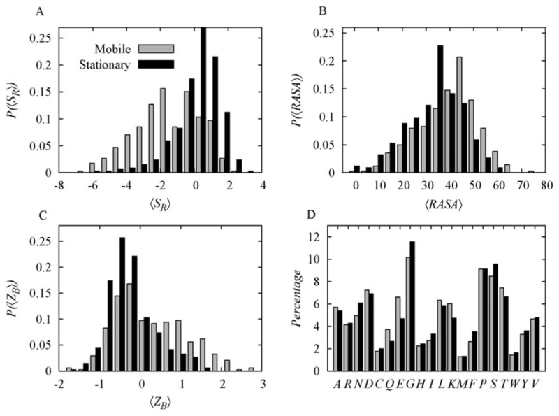
A. 〈S_R〉 separation between mobile and stationary loops (p-value = 2.2 × 10⁻³⁵). B. 〈RASA〉 separation between mobile and static stationary loops (p-value = 1.63 × 10⁻¹⁷). C. 〈Z_B〉 separation between mobile and stationary loops (p-value = 1.6 × 10⁻⁸). D. 〈Z_B〉 Residual composition comparison analysis between mobile loops and stationary loops (p-value = 0.47). All the p-values were calculated by the Wilcoxon rank-sum test.

Since the features also correlate amongst themselves, the performance of the SVM cannot simply be the sum of the correlations of the features with 〈Δ〉. The relative importance of the features in the SVM can be assessed using the f-score²⁷, which can quantitatively rank the discriminative power: a feature with higher f-score has better discriminative power. 〈S_R〉 has the highest f-score of 0.5, which is followed by 〈Z_B〉 with an f-score of 0.24 and 〈RASA〉 with 0.16. This indicates that all three features contribute substantially to the performance of the SVM. The order based on f-score is the same as the order based on correlation with 〈Δ〉 (Table 1). Nonetheless, although 〈S_R〉 and 〈Z_B〉 have similar (absolute) correlation coefficients, their f-scores differ more than a factor 2, reflecting the dependence between these two features.

Flexibility Prediction with SVM

With 〈S_R〉, 〈RASA〉 and 〈Z_B〉 as features, we tested the SVM performance with the four kernel functions in LIBSVM. The prediction accuracies for the BM2 loops, using the 4-fold cross validation as described in the Methods, are 72.1%, 71.1%, 75.3%, and 68.9% for the linear, polynomial, radial basis, and sigmoid kernel functions, respectively. Since the radial basis clearly performed best, we used it for the remaining analyses and predictions in this section. The discriminant score was used to calculate a receiver operating characteristic (ROC) curve and the area under the curve (AUC) value. The average AUC was 0.79 with a standard deviation of 0.03. The averaged ROC curve is shown in Figure 2 (in black), indicating that the SVM predicts the mobility of loops considerably better than random (AUC = 0.5). It is interesting to note that the first 16 predictions were all false positives, as indicated by the horizontal section at the beginning of the ROC curve. These stationary loops all have unfavorable backbone dihedral angles; their 〈S_R〉 are lower than −2 (the average for stationary loops is 0.7), which caused them to be incorrectly predicted as flexible.

Figure 2.

SVM loop-level flexibility prediction accuracy for various levels of confidence cutoffs. The AUC of random prediction is 0.5. The AUC is 0.79 with default cutoff of 0.5. Average ROC curves with confidence cutoffs at 0.6 with 154 loops, 0.7 with 126 loops, and 0.8 with 64 loops are also shown, and they correspond to AUC of 0.80, 0.81, and 0.83 respectively.

As a second assessment of the SVM, we define the accuracy of a prediction as the number of correct predictions (true positives + true negatives) divided by the total number of predictions (true negatives + false negatives + true positives + true negatives):

$$\mathit{accuracy}=\frac{TP+TN}{TN+FN+TP+FP}$$ (4)

With the default discriminant score cutoff of 0.5 for the SVM, we achieved an accuracy of 75.3%, much higher than the baseline accuracy of 50%.

The SVM also reports a quantitative measure for the confidence of its predictions, referred to as the confidence probability. The confidence probability allows a confidence cutoff to be set such that predictions are accepted only when the confidence probability is higher than the cutoff. Indeed, the accuracy and AUC both increase when the predictions are restricted to higher confidence probability cutoffs. The prediction accuracy improves as a higher confident cutoff is applied, as is shown in Figure 2. For example, a confidence probability cutoff of 0.7 yields an accuracy of 80.5% and AUC of 0.81.

We also investigated the difference in performance of the SVM between interfacial loops and non-interfacial loops. We separated the 848 surface loops into two classes, 237 interfacial loops and 611 non-interfacial loops, and followed the training and testing procedures described in the methods for these two groups separately. The AUC is 0.71 ± 0.01 for the interfacial loops and 0.80 ± 0.01 for the non-interfacial loops, indicating that the predictability of SVM is affected by the binding partner proteins, which suggests that protein surface loop mobility is also affected by the binding partner proteins. Furthermore, we trained a new SVM using the same three features to distinguish between interfacial and non-interfacial loops. For this test, we randomly selected 75% of interfacial loops and 75% of non-interfacial loops for training and the rest of 25% were used for testing. The AUC was 0.55 ± 0.01 and the average prediction accuracy was 63% ± 2.2%. This is only slightly better than random (AUC = 0.5 and accuracy = 61%), indicating that the features we used are not promising in the prediction of protein-protein binding interface.

In addition to use the SVM to predict the mobility of entire loops, we also attempted to predict the conformational change of individual residues. Such knowledge would allow one to selectively search the backbone conformational space in protein-protein docking applications. We restricted the dataset to the 3482 residues in the 339 mobile loops, classified as mobile (Δ_i > 30, 2146 residues) or stationary (Δ_i ≤ 30, 1335 residues). Using the SVM with the residue-specific features S_R, RASA and Z_B, we performed 10 repeated tests by randomly picking 75% loops in the mobile set and 75% loops in the stationary set for training, and the rest of 25% for testing. Our average accuracy was 68% ± 1.8 % (compared with the baseline 61.3%) and average AUC was of 0.72 ± 0.04 (compared with the baseline 0.5). We also tested hydrophobicity and molecular weight of each residue as one of the SVM features, but their inclusions did not improve the prediction accuracy or AUC.

Validation test on an independent dataset

As an independent test, we applied the SVM to the unbound structures that were newly added to Benchmark 3.0²⁸ and Benchmark 4.0²⁹ (BM3+BM4 includes 149 unbound structures from which 512 loops were extracted). Training with the loops of BM2 and using the radial basis kernel, the prediction accuracy for the independent set BM3+BM4 is 70.5% compared with 75.3% for the BM2 loops alone using 4-fold cross-validation. This moderate decrease in performance is likely due to the BM3+BM4 loops being harder to predict: when we train and test on BM3+BM4 loops, using 4-fold cross-validation and the radial basis kernel, we obtain an accuracy of 69.7%, which represents a similar decrease in performance.

Whereas we observed a 6% difference in performance between the best and worst performing kernel functions for 4-fold cross-validation on the BM2 loops, this difference is reduced to 3% when testing using the BM3+BM4 loops. We obtained accuracies of 69.1%, 71.1%, 70.5%, and 69.2% for linear, polynomial, radial basis, and sigmoid, respectively (Supplementary table 4). Note that here the radial basis is the second best performing kernel function. The differences among the four kernels, however, are small.

Application to the Ras superfamily of proteins

The Ras superfamily is a well known family of molecular switches in signal transduction that control cell growth and differentiation by alternating between the activated (GTP bound) and inactivated (GDP-bound) forms.^30–32 The docking benchmark version 2.0 contains 11 complexes that involve members from the Ras superfamily, and here we use this set to further illustrate the behavior and performance of our method for loop flexibility prediction. We first give a detailed analysis of the H-Ras protein binding to RasGAP, followed by comparison with other proteins from the Ras superfamily: Ras, Ran, Rac and Cdc42.

H-Ras forms a complex with the GTPase activating protein RasGAP. The Unbound H-Ras protein is the activated form, bound with a GTP analog GDPCP, and the H-Ras protein bound to RasGAP is in the inactivated form with GDP.³⁰ Figures 3 and 4 illustrate the conformational changes of these loops upon binding RasGAP. Switch I (loop 1) and Switch II (loop 2) are involved in the binding process, and indeed show large differences between the bound and unbound form. Loop 4 is not in the interface, but does show modest differences between the bound and unbound forms. Loops 3 and 5 are stationary. Figure 4 shows the S_R, RASA, and Z_B features for the unbound structure, as well as the measure for loop mobility, Δ. S_R shows highly unlikely backbone conformations for Switch I and Switch II, with 4 and 6 instances of S_R = S_Rmin for switch I and switch II respectively, and high Z_B values. These values indicate a high probability of these loops being flexible, and are consistent with the observed Δ’s. Loop 4 is classified as a mobile loop, although the RMSD calculation after structural alignment is low (0.55 Å). The motion of this loop corresponds to the inversion of two consecutive backbone dihedrals, which results in large Δ but small RMSD.

Figure 3.

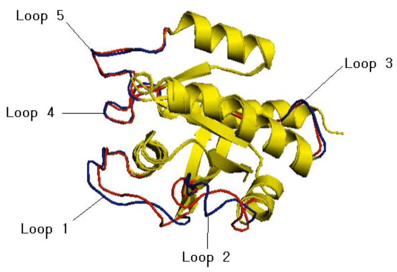
Superimposed unbound form (loops in red, PDB code 6Q21, chain D) and bound form (loops in blue, PDB code 1WQ1 chain R) of H-Ras. Figure generated using PyMOL (www.pymol.org). loop 1 (switch I: residue number 30–38), loop 2 (switch II: residue number 60–67), loop 3 (residue number 105–110), loop 4 (residue number 117–126) and loop 5 (residue number 145–151. The residue numbers listed refer to the numbering of the unbound structure.

Figure 4.

Conformational change and values of the features used for the SVM of H-Ras complexes with Ras GAP. Loop 1 and loop 2 correspond to Switch I and Switch II, respectively.

We trained an SVM as described in the previous section, using the set of loops extracted from BM2 for training, excluding all loops from the Ras superfamily. We then applied the SVM to the loops of all proteins from the Ras superfamily in our database. The SVM correctly predicts H-Ras loops 1, 2 and 4 to be mobile, and loops 3 and 5 to be stationary.

We investigated the features at the residue level in detail to gain a better understanding of the mobility of switch I and switch II. Switch I is composed of 9 residues (Supplementary table 2), 4 of which have S_R = S_Rmin in the unbound protein (shown in bold): D-E-Y-D-P-T-I-E-D. Upon binding, the following changes in Ramachandran angles Δ are found: 30D:174, 31E:154, 33D:175 and 35T:241. Given the overall loop motion, it is perhaps not surprising to note that some residues adjacent to these 4 residues also show a large degree of motion upon binding. Indeed, the adjacent residues with S_R values 32Y:0.65, 36I:2.82 have Δ values of 32Y:149, 36I:169. However, 34P shows a Δ of only 31 degrees, despite being flanked by two residues with S_R = S_Rmin. This is caused by the rigidity provided by Proline’s native backbone restriction. The switch II loop is composed of 8 residues, of which 6 residues have S_R = S_Rmin: (G-Q-E-E-Y-S-A-M). Again, most of these residues show large values for Δ, as well as those residues flanked by residues with S_R = S_Rmin. This observation, that mobile loops may contain some residues of which S_R does not suggest loop motion, is consistent with the superior predictive power of loop-averaged features over residue-level features for loop motion.

We applied the SVM to the remaining Ras proteins from docking benchmark 2.0. Table 2 presents the results on Switch I and Switch II, since only these loops are involved in the binding process. The SVM predicts the flexibility of 92.8% of the given Ras superfamily loops correctly, which is higher than the 75.3% prediction accuracy using the entire set of loops, as described in the previous sections. Interestingly, the mobility of Switch II of Ran depends on the binding partner: with RCC1 the loop is mobile, while it is stationary with nuclear transport factor 2. The SVM prediction, however, is based solely on the unbound structure of Ran, which therefore results in one wrong prediction. Also for H-Ras we have two complexes. But in those cases, we assigned two different unbound structures for the Ras protein when we originally constructed the docking benchmark 2.0, due to the different GTP analogs in the structures. One unbound H-Ras structure (PDB code 821P) binds GTN. Its Switch I is classified as a stationary loop when compared with both complex structures (PDB code 1WQ1 and 1HE8), and our SVM correctly predicted so, based on the high S_R scores (0.94±1.73) and low Z_B values (−0.17±0.49) for the residues in this loop. The other unbound Ras structure (6Q21) binds GCP. Its Switch I is classified as a flexible loop when compared with both complex structures, and our SVM also correctly predicted so, based on the much lower S_R scores (−1.82±5.86) and higher Z_B values (1.47±0.49) for the residues in this loop. The two different unbound Ras structures have the same protein sequence but different cofactors, indicating that cofactors can affect the flexibility of protein loops significantly, and that this is accurately recognized by our SVM.

Table 2.

SVM predictions for Switch I and Switch II flexibility of the Ras superfamily proteins.

Complex		Switch I			Switch II
Ras protein	Binding Partner	Mobile?	Prediction	Interface?	Mobile?	Prediction	Interface?
H-Ras	Ras GAP	Yes	Correct	Yes	Yes	Correct	Yes
H-Ras	PIP3 Kinase	No	Correct	Yes	Yes	Correct	Yes
Rac	p67 Phox	Yes	Correct	Yes	No	Correct	No
Rac	Pseudomonas toxin GAP domain	Yes	Correct	Yes	No	Correct	Yes
Rac	Arfaptin	Yes	Correct	Yes	No	Correct	No
Ran	RCC1	Not a loop	N/A	No	Yes	Correct	Yes
Ran	Nuclear transport factor 2	Not a loop	N/A	No	No	Incorrect	No
CDC42	CDC42 GAP	Yes	Correct	Yes	No	Correct	Yes

Finally, we performed prediction on the binding partners of the Ras superfamily proteins. There are a total of 43 surface loops, including 18 mobile loops and 21 stationary loops (4 loops are classified undefined). 14 out of 18 mobile loops were correctly predicted and 15 out of 21 stationary loops were correctly predicted. This corresponds to a prediction accuracy of 74.4%, which is similar to the prediction accuracy of the entire set of proteins. Supplementary table 3 summarizes the SVM prediction results for Ras protein binding partners.

Conclusions

The most recent evaluation report on the 4th CAPRI showed that protein-protein docking is an active research field.³³ The current rigid-body docking methods have a limited performance on blind docking cases that are involved with conformational changes.^34–36 In order to include loop flexibility in protein-protein docking algorithms in a computationally efficient way, we developed a machine learning algorithm based on SVM to predict which loops on a protein surface will change conformation upon protein-protein binding. Three features of the unbound protein, 〈S_R〉, 〈RASA〉, and 〈Z_B〉, led to an effective SVM with high accuracy: we obtained a prediction accuracy of 75.3% using cross–validation, and 70.5% when tested on an independent dataset. The three features were not as effective in discriminating loops in binding interface from other surface loops. Thus, our method can be combined with interface prediction methods, such as the PINUP³⁷ and ACF³⁶ methods, to further increase the tractability of flexible protein-protein docking.

References

- 1.Lensink MF, Mendez R, Wodak SJ. Docking and scoring protein complexes: CAPRI 3rd Edition. Proteins. 2007;69(4):704–718. doi: 10.1002/prot.21804. [DOI] [PubMed] [Google Scholar]
- 2.Lensink MF, Wodak SJ. Blind predictions of protein interfaces by docking calculations in CAPRI. Proteins. 78(15):3085–3095. doi: 10.1002/prot.22850. [DOI] [PubMed] [Google Scholar]
- 3.Dunbrack RL, Jr, Karplus M. Backbone-dependent rotamer library for proteins. Application to side-chain prediction. J Mol Biol. 1993;230(2):543–574. doi: 10.1006/jmbi.1993.1170. [DOI] [PubMed] [Google Scholar]
- 4.Bower MJ, Cohen FE, Dunbrack RL., Jr Prediction of protein side-chain rotamers from a backbone-dependent rotamer library: a new homology modeling tool. J Mol Biol. 1997;267(5):1268–1282. doi: 10.1006/jmbi.1997.0926. [DOI] [PubMed] [Google Scholar]
- 5.Pal D, Chakrabarti P. On residues in the disallowed region of the Ramachandran map. Biopolymers. 2002;63(3):195–206. doi: 10.1002/bip.10051. [DOI] [PubMed] [Google Scholar]
- 6.Zhang CT, Zhang R. Skewed distribution of protein secondary structure contents over the conformational triangle. Protein Eng. 1999;12(10):807–810. doi: 10.1093/protein/12.10.807. [DOI] [PubMed] [Google Scholar]
- 7.Lo Conte L, Chothia C, Janin J. The atomic structure of protein-protein recognition sites. J Mol Biol. 1999;285(5):2177–2198. doi: 10.1006/jmbi.1998.2439. [DOI] [PubMed] [Google Scholar]
- 8.Bonvin AM. Flexible protein-protein docking. Curr Opin Struct Biol. 2006;16(2):194–200. doi: 10.1016/j.sbi.2006.02.002. [DOI] [PubMed] [Google Scholar]
- 9.Kuznetsov IB. Ordered conformational change in the protein backbone: Prediction of conformationally variable positions from sequence and low-resolution structural data. Proteins. 2008 doi: 10.1002/prot.21899. [DOI] [PubMed] [Google Scholar]
- 10.Andrusier N, Mashiach E, Nussinov R, Wolfson HJ. Principles of flexible protein-protein docking. Proteins. 2008;73(2):271–289. doi: 10.1002/prot.22170. [DOI] [PMC free article] [PubMed] [Google Scholar]
- 11.Wang C, Bradley P, Baker D. Protein-protein docking with backbone flexibility. J Mol Biol. 2007;373(2):503–519. doi: 10.1016/j.jmb.2007.07.050. [DOI] [PubMed] [Google Scholar]
- 12.Mashiach E, Nussinov R, Wolfson HJ. FiberDock: Flexible induced-fit backbone refinement in molecular docking. Proteins. 78(6):1503–1519. doi: 10.1002/prot.22668. [DOI] [PMC free article] [PubMed] [Google Scholar]
- 13.Bastard K, Prevost C, Zacharias M. Accounting for loop flexibility during protein-protein docking. Proteins. 2006;62(4):956–969. doi: 10.1002/prot.20770. [DOI] [PubMed] [Google Scholar]
- 14.Noble WS. What is a support vector machine? Nat Biotechnol. 2006;24(12):1565–1567. doi: 10.1038/nbt1206-1565. [DOI] [PubMed] [Google Scholar]
- 15.Mintseris J, Wiehe K, Pierce B, Anderson R, Chen R, Janin J, Weng Z. Protein-Protein Docking Benchmark 2. 0: an update. Proteins. 2005;60(2):214–216. doi: 10.1002/prot.20560. [DOI] [PubMed] [Google Scholar]
- 16.Wang G, Arthur JW, Dundbrack S2C: A database correlating sequence and atomic coordinate numbering in the Protein Data Bank. 2002 http://www.fccc.edu/research/labs/dubrack/s2c.
- 17.Frishman D, Argos P. Knowledge-based protein secondary structure assignment. Proteins. 1995;23(4):566–579. doi: 10.1002/prot.340230412. [DOI] [PubMed] [Google Scholar]
- 18.Hubbard SJ, Thronton JM. NACCESS 2.1.1. 1993. [Google Scholar]
- 19.Word J. All-atom small-probe contact surface analysis: an information-rich description of molecular goodness-of-fit. Durham: Duke University; 2000. p. 274. [Google Scholar]
- 20.Chih-Chung C, Chih-Jen L. A library for support vector machines. 2001. [Google Scholar]
- 21.Hubbard SJ, Campbell SF, Thornton JM. Molecular recognition. Conformational analysis of limited proteolytic sites and serine proteinase protein inhibitors. J Mol Biol. 1991;220(2):507–530. doi: 10.1016/0022-2836(91)90027-4. [DOI] [PubMed] [Google Scholar]
- 22.Lovell SC, Davis IW, Arendall WB, 3rd, de Bakker PI, Word JM, Prisant MG, Richardson JS, Richardson DC. Structure validation by Calpha geometry: phi,psi and Cbeta deviation. Proteins. 2003;50(3):437–450. doi: 10.1002/prot.10286. [DOI] [PubMed] [Google Scholar]
- 23.Smith LJ, Bolin KA, Schwalbe H, MacArthur MW, Thornton JM, Dobson CM. Analysis of main chain torsion angles in proteins: prediction of NMR coupling constants for native and random coil conformations. J Mol Biol. 1996;255(3):494–506. doi: 10.1006/jmbi.1996.0041. [DOI] [PubMed] [Google Scholar]
- 24.Anderson RJ, Weng Z, Campbell RK, Jiang X. Main-chain conformational tendencies of amino acids. Proteins. 2005;60(4):679–689. doi: 10.1002/prot.20530. [DOI] [PubMed] [Google Scholar]
- 25.Breiman L, Schapire E. Random forests. 2001. pp. 5–23. [Google Scholar]
- 26.Liaw A, Wiener M. Classification and Regression by randomForest. R News. 2002;2:18–22. [Google Scholar]
- 27.Chen YW, Lin CJ. Combining {SVM}s with various feature selection strategies. In: Guyon ISG, Nikravesh M, Zadeh L, editors. Feature extraction, foundations and applications. Springer; 2006. [Google Scholar]
- 28.Hwang H, Pierce B, Mintseris J, Janin J, Weng Z. Protein-protein docking benchmark version 3. 0. Proteins. 2008;73(3):705–709. doi: 10.1002/prot.22106. [DOI] [PMC free article] [PubMed] [Google Scholar]
- 29.Hwang H, Vreven T, Janin J, Weng Z. Protein-protein docking benchmark version 4.0. Proteins. 78(15):3111–3114. doi: 10.1002/prot.22830. [DOI] [PMC free article] [PubMed] [Google Scholar]
- 30.Milburn MV, Tong L, deVos AM, Brunger A, Yamaizumi Z, Nishimura S, Kim SH. Molecular switch for signal transduction: structural differences between active and inactive forms of protooncogenic ras proteins. Science. 1990;247(4945):939–945. doi: 10.1126/science.2406906. [DOI] [PubMed] [Google Scholar]
- 31.Scheffzek K, Ahmadian MR, Kabsch W, Wiesmuller L, Lautwein A, Schmitz F, Wittinghofer A. The Ras-RasGAP complex: structural basis for GTPase activation and its loss in oncogenic Ras mutants. Science. 1997;277(5324):333–338. doi: 10.1126/science.277.5324.333. [DOI] [PubMed] [Google Scholar]
- 32.Ehrhardt A, Ehrhardt GR, Guo X, Schrader JW. Ras and relatives--job sharing and networking keep an old family together. Exp Hematol. 2002;30(10):1089–1106. doi: 10.1016/s0301-472x(02)00904-9. [DOI] [PubMed] [Google Scholar]
- 33.Lensink MF, Wodak SJ. Docking and scoring protein interactions: CAPRI 2009. Proteins. 78(15):3073–3084. doi: 10.1002/prot.22818. [DOI] [PubMed] [Google Scholar]
- 34.Wiehe K, Pierce B, Tong WW, Hwang H, Mintseris J, Weng Z. The performance ofZDOCK and ZRANK in rounds 6–11 of CAPRI. Proteins. 2007;69(4):719–725. doi: 10.1002/prot.21747. [DOI] [PubMed] [Google Scholar]
- 35.Wiehe K, Pierce B, Mintseris J, Tong WW, Anderson R, Chen R, Weng Z. ZDOCK and RDOCK performance in CAPRI rounds 3, 4, and 5. Proteins. 2005;60(2):207–213. doi: 10.1002/prot.20559. [DOI] [PubMed] [Google Scholar]
- 36.Hwang H, Vreven T, Pierce BG, Hung JH, Weng Z. Performance of ZDOCK and ZRANK in CAPRI rounds 13–19. Proteins. 78(15):3104–3110. doi: 10.1002/prot.22764. [DOI] [PMC free article] [PubMed] [Google Scholar]
- 37.Liang S, Zhang C, Liu S, Zhou Y. Protein binding site prediction using an empirical scoring function. Nucleic Acids Res. 2006;34(13):3698–3707. doi: 10.1093/nar/gkl454. [DOI] [PMC free article] [PubMed] [Google Scholar]
Associated Data
This section collects any data citations, data availability statements, or supplementary materials included in this article.