Venous Oxygenation Mapping using Velocity-Selective Excitation and Arterial Nulling (VSEAN)

Abstract

A new MRI technique to map the oxygenation of venous blood is presented. The method uses velocity-selective excitation and arterial nulling pulses, combined with phase sensitive signal detection to isolate the venous blood signal. The T₂ of this signal along with a T₂-Y calibration curve yields estimates of venous oxygenation in situ. Results from phantoms and healthy human subjects under normoxic and hypoxic conditions are shown, and venous saturation levels estimated from both sagittal sinus and grey matter based ROIs are compared to the related techniques TRUST and QUIXOTIC. In addition, combined with an additional scan without arterial nulling pulses, the oxygen saturation level on arterial side can also be estimated.

Introduction

After stroke, in hypoperfused but potentially salvable regions referred as the ischemic penumbra, the brain tissue is perfused at a level where its function is impaired but morphological integrity remains (1). This hemodynamic state is characterized by reduced cerebral blood flow with increased Oxygen Extraction Fraction (OEF) to maintain vital oxygen metabolism (2). The penumbra was originally identified and defined as high OEF regions by Positron Emission Tomography (PET) imaging in 1979 (3). The mismatched regions from Diffusion Weighted Imaging (DWI) and Perfusion Weighted Imaging (PWI) are widely used as a practical surrogate to identify the penumbra that may be amenable to therapies in acute and ischemic stroke due to its relatively easy accessibility compared to PET. However, recent studies comparing DWI/PWI with PET (4–7) suggest that the MRI DWI-PWI mismatched regions cannot clearly differentiate true penumbra from oligemia, and the amount of tissue at risk is often overestimated from DWI-PWI mismatch. This provides motivation for returning to OEF as a better means of identifying the true penumbra.

In studies of brain function, the uncoupling of flow and oxygen metabolism gives rise to Blood Oxygenation Level Dependent (BOLD) effect (8). However, due to the complex dynamics of blood flow, blood volume, oxygen metabolism changes, etc., researchers are looking into more direct ways of measuring cerebral metabolic rate of O₂ (CMRO₂) noninvasively, such as calibrated (9) or quantitative BOLD (qBOLD) (10–12).

CMRO₂ can be calculated from OEF, CBF (cerebral blood flow) and arterial oxygen content (CaO₂): CMRO₂ = CaO₂*CBF*OEF, where OEF can be estimated from arterial and venous blood oxygenation difference. Research focusing on measurement of blood oxygenation with MRI includes: measuring the susceptibility caused by deoxygenated hemoglobin and converting it into venous oxygenation (13–15); measuring R₂′ (10,11) or ΔR₂′ (12) and estimating venous oxygenation through the qBOLD model (16,17); and measuring blood T₂/T₂* and converting it into oxygenation level through a model or calibration curve (18–23). These methods have their own challenges and limitations: methods based on susceptibility are limited to relatively large and straight vessels that are fully resolved by the imaging process; the qBOLD method is suitable for in situ measurement, but the model is complicated with a large number of parameters to fit (10,11), and high signal-to-noise ratio (SNR) is necessary to produce good fitting results (24), or it requires injection of intravascular contrast agent (12); methods based on T₂ measurement can be applied both in situ or in large vessels, but a good separation of blood from surrounding tissues is critical to avoid partial volume effects.

Among the T₂-based methods, experiments were successfully carried out in large vessels (18,21) and the partial volume effect was further reduced by using magnetization preparation and subtraction methods such as in TRUST (25). However, spatial information is largely lost in measurements from big vessels; and measurements from local draining veins, or in situ are desired (19,20) where the partial volume effect is most challenging.

Recently the QUIXOTIC method introduced by Bolar et al (26,27) provides insight into separating the blood and the tissue signal. It uses a velocity-selective (VS) spin labeling technique to separate accelerating venous blood from decelerating arterial blood and static tissue. However, since the flow-sensitive gradients are turned on in the tag condition but not in the control condition, the signal difference from diffusion attenuation, especially that from cerebrospinal fluid (CSF), may contaminate the venous signal of interest (27), and there may be interference from eddy current effects. In addition, to suppress the arterial signal, a global inversion pulse is applied which also attenuates the signal of venous blood and brain tissue, from which the venous signal originates and the subtraction scheme has relatively low temporal efficiency.

In this study, a new technique referred as Velocity-Selective Excitation with Arterial Nulling (VSEAN) (28), is demonstrated to help address these issues with a focus on isolating the venous blood signal and conducting T₂ measurements. The modeling and calibration involved in converting T₂ values to blood oxygen saturation has been investigating by others (23,29–31), and is outside of the scope of this study.

Theory

Nulling of arterial blood

To accurately estimate the venous oxygenation using T₂ based methods, the venous blood signal has to be separated clearly from other signal sources such as the brain tissue, CSF and arterial blood. To remove the arterial blood signal, a slab-selective inversion pulse is applied below the imaging plane, and a delay time TI, which is set to coincide with the null point of blood longitudinal magnetization (M_z), allows for the inverted bolus of arterial blood to travel to the imaging plane. At the null point, a portion of the bolus occupies the arterial side of the vasculature and thus does not contribute to the observed signal. Another portion may enter capillaries or exchange with tissue water, but would not be excited by the velocity-selective excitation (VSE, see below). A third portion may enter the venous circulation, but this portion is likely to be negligible due to fast exchange between blood and tissue water pools (32,33), and the arterial and capillary transit times. Since the inversion pulse is slab-selective, the spins of tissue and venous blood in the imaging slice is unperturbed by the inversion, providing stronger venous signal relative to that of QUIXOTIC (Figure 1).

FIG. 1.

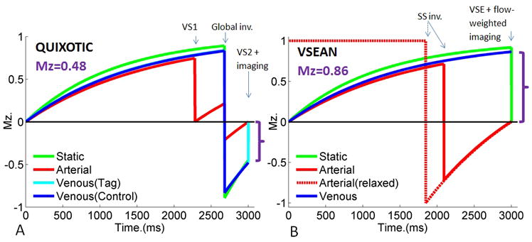
Simulated magnetization evolution of venous signal using A) QUIXOTIC, B) VSEAN with T_1arterial=1664ms, T_1venous=1500ms, T_1tissue=1200ms and TR=3s. Magnetizations indicated by purple brackets show the magnitude of the QUIXOTIC and VSEAN signals, respectively.

Velocity-Selective Excitation (VSE)

At the null point of arterial blood, a VSE pulse module is applied to excite the moving spins, without generating signal from static and slow flowing spins, including brain tissue, CSF, and the blood in capillaries. Since the static tissue signal is usually much stronger than the blood signal of interest, an efficient suppression of the static tissue is critical for in situ measurements. With conventional VS pulses, the moving spins that accumulate nπ phase are tipped back to the longitudinal axis, generating a cosine-shaped M_z response with respect to velocity: M_z=M₀cos(βv), referred as “cos” modulation (Figure 2), where β is the flow moment controlled by flow-weighting gradients. With an extra ±π/2 phase added to the last tip-up portion in VS module (34), the moving spins that accumulate 2nπ±π/2 phase are tipped back to the longitudinal axis instead, leaving the spins that accumulate nπ phase, including the static tissue, on the transverse plane to be destroyed by a strong gradient spoiler, therefore a sine-shaped M_z profile is generated: M_z=M₀sin(βv), referred as “sin” modulation. This modification can be made on VS pulses using BIR4-based (34), dual-sech (35) or hard pulses (36), in this study we chose BIR4-based pulses for both B₀ and B₁ insensitivity (37). The VSE pulse train and spin evolution process are illustrated in Figure 2. We define the lowest velocity that generates π/2 phase shift as v_e for convenience.

FIG. 2.

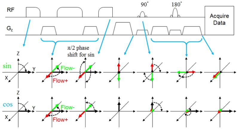
Illustration of the sequence (only VSE and imaging parts) and spin evolution diagram in VSEAN. Red and green arrows depict spins that undergo ±π/2 phase shift due to flow through velocity encoding gradients. Black arrows depict static spins. Note that for “sin” modulation, flowing spins in both directions finish aligned along +X, while under “cos” modulation, static spins are aligned along +Y.

Note that spins moving in opposite directions will accumulate phases of 2nπ±π/2, and will be tipped onto +Z or −Z axis accordingly, and their signals tend to cancel if they are in the same voxel. In addition, the steep velocity dependency around zero velocity makes it sensitive to slow motion. To avoid these problems, another VSE module can be applied to generate a sine-squared profile: M_z= M₀sin²(βv) which has a flat response around zero velocity, and should therefore be robust against slow motion. In addition, the phases of spins that are moving in opposite directions will have the same sign and thus avoid signal cancellation. However, the “sin²”excitation signal is attenuated, given a uniform velocity distribution, it generates π/4=0.785 of the signal with “sin” excitation.

Flow Signal Separation by Projection

Instead of applying the same “sin” modulated VSE pulse module twice, the second module is incorporated into image acquisition by adding flow-weighting gradients with the same flow moment as in the VSE preparation pulses. This reduces signal loss due to T₂ decay as well as RF power. More importantly, the π/2 phase difference between the static and moving signals with desired velocity is preserved (shown in Figure 2), thereby allowing the separation of the moving signal from residual static signal. First, a reference phase for static tissue was estimated from a “cos” modulated signal where the static tissue signal is dominant. The “sin” modulated signal is then projected onto this phase reference axis, and separated into two components: the residual static tissue signal aligned with the reference axis, a “real” component; and the flow signal of interest with a π/2 phase shift, the “imaginary” component, which has a net sin² dependence on velocity as described above. In principle, the reference phase images can be acquired with no VSE preparation at all, however, by using the “cos” modulated VSE pulse train, the gradients are exactly the same as in the “sin” modulated VSE pulse train, and the method should be robust against eddy current effects.

T₂ measurement and Oxygenation Estimation

The T₂ measurement of venous blood and translation to oxygen saturation is independent of the venous signal separation process. There are several methods available: 1) T₂ preparation; 2) multiple single-echo spin-echo (SE) acquisitions; and 3) multi-echo SE acquisition. The T₂ preparation method is in principle insensitive to flow effect, but the temporal efficiency and resolution is relatively low, and signal fluctuations across TR periods may introduce errors. The multiple single-echo SE method has the same issues, and it could be affected by flow effects. The multi-echo SE acquisition method provides better temporal efficiency and robustness against fluctuations across TR’s, but it may be affected by flow effects and stimulated echoes. In this study, we used T₂ preparation method due to its simplicity and robustness in presence of flow, but continue to explore multi-echo SE methods for their high temporal efficiency. The measured T₂ values were then translated to blood oxygen saturation via a T₂-Y calibration curve acquired from bovine blood sample in vitro at 3T (29), where Y is the blood oxygen saturation.

Pulse sequence

The layout of the VSEAN sequence is shown in Figure 3.

FIG. 3.

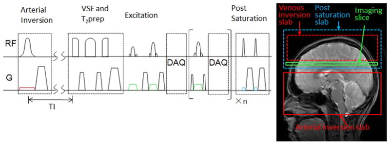
VSEAN sequence diagram and tagging scheme.

Arterial nulling

A slab-selective hyperbolic secant pulse (38) is used to invert a bolus of arterial blood below the imaging plane, followed by a gradient spoiler to destroy residual transverse magnetization and a delay time TI. In this study we used PICORE-type (39) preparation: a slab selective pulse is referred to as an Arterial-Nulling (AN) experiment; and a nonselective off-resonance pulse (the PICORE control) is referred to as a non-Arterial-Nulling (non-AN) experiment. The latter compensates for Magnetization Transfer (MT) and slice profile effects, and allows for separation of arterial and venous components. If one wants to reduce the contribution from the venous blood above the imaging slice, preparations such as EPISTAR (40), or FAIR (41,42) can be used.

Velocity-selective excitation

A BIR4-based VSE pulse module (34) is applied at the null point of arterial blood, with flow-weighting gradients between the RF pulses. The parameters (37) of the BIR-4 pulse are: pulse length 6ms; ω_max=42.52KHz; zeta=43.58; tan(κ)=69.65; and two gaps of 1–8 milliseconds follow the gradients to reduce possible interference between eddy currents and RF pulses. The last BIR1 subpulse has 0 or ±π/2 phase shift in addition to the original phase to generate “cos” or “sin” modulation accordingly. In principle either +π/2 or −π/2 phase shift should work. However, in our implementation, −π/2 phase shift gave better static spin suppression and was used in this study.

T₂ preparation (T₂prep)

We modified the original BIR4-based T₂ preparation pulses (43) by merging it into the VSE module: two controllable gaps were inserted between the first and last BIR1 subpulses and the flow-weighting gradient to generate desired T₂-weightings without perturbing the flow-weighting gradients. The excitation pulses are applied immediately after the spoilers at the end of this VSE/T₂prep module to minimize the T₁ recovery of the static tissue signal. This VSE/T₂prep combined design also reduces RF power. The scan repetition time was fixed in this study, so the spins experienced different T₁ recovery times at different effective echo times (eTE’s). The error from neglecting this effect was found by simulation to be less than 0.6%.

Image acquisition

A slice-selective excitation pulse is followed by refocusing pulses to generate spin echoes. In this study, we used sinc and dual-sech refocusing pulses in different experiments, the former for its short echo time and the latter for its B₁ insensitivity and better slice profile (44). The flow-weighting gradients are around the first refocusing pulse.

Post-saturation pulses

After the image acquisition, a set of saturation pulses are applied to reset the spins for the next TR, either locally or “globally”. In principle, a global non-selective saturation pulse could reset the magnetization of all spins, thus ensuring a well-characterized spin history, independent of inflow into the inversion slab. However, in a typical whole body scanner, the transmit RF coil extends only to the upper part of the torso, and our measurements indicate that after non-selective saturation, unperturbed blood reaches the brain in approximately 1s. Thus, given the timing of our pulse sequence, the use of non-selective saturation would confound the magnetization history of arterial blood due to mixing of saturated and fully-relaxed blood, leaving the null point poorly-defined. In this study the saturation pulses were applied locally, above the arterial inversion slab, including the imaging slice and the brain tissue above. By applying the saturation pulses locally, fully-relaxed arterial blood flows into the inversion slab. If the inversion slab is refreshed with relaxed blood prior to inversion, this provides a well-defined null point, and also allows for the use of a longer TI, in turn allowing more time for arterial filling by the inverted blood. This condition is met if the inversion slab is refreshed in a time (TR-TI), which in our experiment is greater than 1.5s, and we believe that this condition is well met in our experiments. Figure 1B shows the arterial magnetization for blood that is saturated (solid red) and relaxes (dashed red) prior to inversion. Our experiment follows the dashed red curve, while for non-selective saturation the net magnetization is somewhere between the red solid and dashed curves.

Experimental setup, data collection and processing

All experiments were performed on a GE Discovery MR750 3T system, using a commercial 8-channel RF coil. Images were complex-reconstructed offline with homemade software, and processed in Matlab (Mathworks, Inc.). For VSEAN data, the signal projection procedure was applied individually for each channel after complex-reconstruction and then combined together: the phase associated with the coil itself is the same for “cos” and “sin” modulated data, and is cancelled after the projection process, so the extracted signals from different coils are in phase with signs, allowing directly summing up together weighted by the coil sensitivities estimated from the “cos” modulated data, which has high SNR. The noise is kept zero-mean since the sign of signal is preserved in combination, in contrast with the Sum of Square (SOS) method. SOS reconstruction was used in QUIXOTIC and TRUST data analysis, where the nonzero means of the noise were removed after subtraction.

When analyzing regions of interest (ROI’s), the T₂ values were calculated pixel-wise. Noisy pixels yielding T₂<0, or T₂>300ms in the flow phantom experiments, and T₂<0 or T₂>150ms in human experiments were discarded. The mean and standard deviation (STD) were then calculated from all the T₂ values. This was referred as “ROI mean±STD” in Table 1 and used to calculate the mean ROI T₂ values in Table 2. The oxygen saturation after T₂-Y conversion was also reported. In the flow phantom experiments, a single T₂ value was also fitted after averaging the signal intensities first in each ROI, for the sample should have identical T₂ value in each ROI. This is referred as “average and fit” in Table 1.

Table 1.

T₂ values measured in flow phantom experiments.

T2 (ms)	ROI	1	2	3	4	5
Stationary	Average and fit	245.2	243.9	234.7	166.4	239.5
	ROI mean±SD	245.5±5.2	243.5±4.0	233.3±3.7	166.1±3.1	239.2±3.8
Circulating	Average and fit	239.5	244.7	219.5	156.8	241.1
	ROI mean±SD	238.6±5.1	242.5±4.9	218.3±8.5	156.8±3.5	241.0±3.9
Circulating w/VSE	Average and fit	233.4	226.3	215.5	N/A	N/A
	ROI mean±SD	233.4±9.4	226.4±10.0	216.2±10.6	N/A	N/A

Table 2.

T₂ values and oxygenation levels measured under normoxia. VSEAN signal intensities in GM are also listed. All numbers are expressed as mean±SD.

Sub. Sex		VSEAN					QUIXOTIC				TRUST
	ROI	GM/WB			SS		GM/WB		SS		SS
		Sig. (%)	T2 (ms)	O2 (%)	T2 (ms)	O2 (%)	T2 (ms)	O2 (%)	T2 (ms)	O2 (%)	T2 (ms)	O2 (%)
1 M	A	0.29±0.15	60.4±25.0	78.3±15.1
	A&V	0.77±0.57	39.1±14.8	65.9±13.2	43.4±6.8	71.9±5.0
	V	0.48±0.53	33.1±18.3	57.1±19.1	41.5±8.0	70.3±5.9	66.2±29.3	80.9±14.3	40.5±13.6	68.4±8.6
2 M	A	0.23±0.24	61.6±31.3	77.2±18.2
	A&V	1.43±1.14	42.4±13.5	69.0±12.9	41.2±5.7	70.4±4.7
	V	1.20±0.99	36.5±14.0	62.6±16.4	37.5±3.8	67.5±3.4	57.2±27.1	76.4±15.0	43.4±13.2	71.3±6.1
3 F	A	0.27±0.16	41.4±21.9	64.5±19.9
	A&V	1.06±0.61	37.1±13.3	64.4±12.6	42.6±13.5	70.0±8.9
	V	0.79±0.56	36.6±16.4	62.2±17.1	38.8±12.6	66.5±10.8	56.3±28.4	74.9±17.1	35.6±9.7	64.6±7.7	34.4±9.6	63.2±8.8
4 M	A	0.17±0.20	59.2±32.7	74.4±21.4
	A&V	1.06±0.78	41.1±17.4	66.6±15.4	38.4±7.8	67.6±6.3
	V	0.89±0.81	35.0±16.1	60.0±18.0	34.9±6.4	64.4±6.5	58.1±29.6	75.3±18.7	34.3±9.9	62.6±11.0	36.8±9.7	64.8±12.3
Mean T2 (ms)	A		55.7±9.6
	V		35.3±1.6		37.6±2.8		59.4±4.6*		38.5±4.2		35.6±1.7

^*T₂ values measured from GM by QUIXOTIC are significantly higher than that by VSEAN (p=0.004).

Experiments using a stationary phantom

The VSE pulse modules were first tested on a stationary gel phantom. The imaging parameters were: FOV=200*200mm, slice thickness=8mm, resolution 64*64, single-slice single SE with spatial-spectral excitation and a sinc 180° refocusing pulse, single-shot spiral readout, v_e set to 2cm/s in the slice-select direction, TE/TR= 18ms/1s, 2 dummy scans followed by 10 acquisitions, the first 4 were “cos” modulated and the rest “sin” modulated, scan time 12s. For comparison, QUIXOTIC data was also collected: the imaging and preparation pulse parameters were the same, no global inversion pulse, only the VS2 module (26) right before the imaging was applied.

The images were averaged across TR’s first. For VSEAN data, the residual “static” and the “moving” signals were extracted as “real” and “imaginary” components accordingly; for QUIXOTIC data, the “moving” signal was calculated from subtraction between the “control” and “tag” images.

Experiments using a rotating phantom

A spherical gel phantom was fixed in a cylindrical plastic case connected by a long rod to a stepper motor in the console room, which can induce controlled rotation about the scanner axis. After a localizer scan, the diameter (D) of the phantom was measured, and the maximum velocity on the edge of the phantom to be v_max=8cm/s, giving an in-plane rotating velocity at radius r of v(r)=2*v_max*r/D. The VSE pulse train was tested with global post-saturation and imaging parameters: axial scan, FOV=200*200mm, 8mm slice thickness, single-slice single SE with sinc 90° and 180° pulses, TE/TR=12ms/3s, 64*64 resolution, single-shot spiral readout, flow-weighting gradients along the A/P direction with v_e=2cm/s, 12 repetitions and 36s for each experiments. For the following 6 experiments, the phantom was stationary in experiments 1 and 2, and rotating through experiments 3–6: 1) no VSE, no flow-weighting gradients in imaging; 2) VSE with “cos” modulation, with flow-weighting gradients in imaging; 3) no VSE, with flow-weighting gradients in imaging; 4) VSE with “cos” modulation, no flow-weighting gradients in imaging; 5) VSE with “sin” modulation, no flow-weighting gradients in imaging; 6) VSE with “sin” modulation, with flow-weighting gradients in imaging.

The images in experiment 1 were used as a phase reference for experiment 3, and those in experiment 2 for experiments 4–6. The magnitude of the images was normalized to their reference scans, and the “static” and “moving” signals were extracted as “real” and “imaginary” components. The data along a horizontal line passing through the center of the phantom gave the VSE profile.

Experiments using a flow phantom

In this experiment, copper sulfate doped water was circulated through a set of plastic hoses connected to a dialyzer (Optiflux F160NR, Fresenius Medical Care), with the flow rate adjusted by a valve. A “U”-loop section of the hose was fixed on top of the dialyzer and a syringe filled with the same solution without flow was also in the FOV. A cross-section image is shown in Figure 6A, with ROI’s shown in Figure 6G: ROI 1 and 2 the big hose, ROI 3 the small hose, ROI 4 the dialyzer, and ROI 5 the syringe. T₂ maps of the phantom were acquired using a BIR4 T₂ preparation pulse under both stationary and circulating conditions; and two sets of VSEAN data were also collected: 1) no flow with “cos” modulated VSE/T₂prep pulse as a reference scan, 6 repetitions and 12s each; and 2) flowing water with “sin” modulated VSE/T₂prep pulse, 18 repetitions and 36s each. The imaging parameters were: FOV=100mm*100mm, slice thickness=8mm, single-slice single echo SE with spatial-spectral excitation and a sinc 180° refocusing pulse, spiral readout with resolution 64*64, TE/TR =18ms/2s, three eTE’s 10/30/70ms in BIR4 T₂prep experiments, 30/50/90ms in VSE/T₂prep experiments, v_e=2cm/s in the slice-select direction. A velocity map in the same plane was collected using a conventional phase contrast sequence with VENC=8cm/s.

FIG. 6.

A. “cos” modulated reference image (magnitude, a.u.); B. Predicted (from A and D) “sin” modulated real components (a.u.); C. Predicted “sin” modulated, imaginary components (a.u.); note that the noise outside the phantom was removed due to the mask used on velocity map; D. Velocity map (cm/s); E. Measured “sin” modulated real components (a.u.); F. Measured “sin” modulated, imaginary components (a.u.); note that this component is rectified across positive and negative flow directions, as expected for a sin² velocity dependence, and both the real and imaginary components closely matched the predicted signal pattern; G. T₂ maps when the phantom was stationary (ms), ROI’s labeled; H. T₂ maps when the phantom was circulating (ms); I. T₂ maps measured with VSE (ms).

The velocity map of the phantom was calculated from the phase difference map and then masked by the magnitude image. We noticed that the measured average velocity in the static syringe was slightly non-zero, presumably due to gradient imperfections, and this value was subtracted from the entire velocity map. Predicted maps of the real and imaginary components of “sin” modulated signal were calculated as follows. The magnitude image of the “cos” modulated signal (stationary) was oversampled and registered to the velocity map, then multiplied with the theoretical velocity excitation profile to give the “real” (sin(π*v/4)cos(π*v/4)) and “imaginary” (sin²(π*v/4)) components. T₂ maps of the flow phantom were calculated by exponential fitting, and average T₂ values were calculated for the ROI’s.

Healthy human volunteer experiments under normoxia

5 healthy human volunteers (4 males, 1 female, age 25–47) were scanned under an IRB-approved protocol. The imaging parameters were: FOV=200mm*200mm, slice thickness=8mm, single-slice SE with spatial-spectral excitation and two slice-selective hyperbolic secant refocusing pulses, single-shot spiral readout with original resolution 32*32, re-gridded to 64*64, TR/TE =3s/28ms, VSE/T₂prep with eTE’s 20/40/80ms, v_e=2cm/s in the slice-select direction, arterial inversion slab thickness 200mm, 25mm below the imaging plane, TI=1150ms assuming T_1b=1664ms (45), slice-selective post-saturation pulses, 2 dummy scans followed by 126 acquisitions including 6 “cos” modulated reference scans at the beginning, scan time 6min 18sec. VSEAN data with AN and non-AN were collected on each subject. Grey Matter masks were acquired using double-inversion prepared sequence with the same resolution except for subject 1, for whom this image was not acquired, and a grey matter mask was calculated from non-AN VSEAN images.

Arterial components were extracted by subtracting the AN data from the non-AN data, and T₂ maps from arterial-only, arterial-and-venous, and venous-only data were calculated. Two ROI’s were chosen to analyze: 1) Grey Matter (GM); and 2) sagittal sinus (SS), shown in Figure 8C. T₂ values in the ROI’s were converted into blood oxygenation levels via a T₂-Y calibration model at 3Tprovided in ref. (29): T₂⁻¹(s⁻¹) = 8.3+33.6*(1−Y)+71.9*(1−Y)², where a similar T₂ measurement was performed by varying the echo times without changing the number of RF pulses and a hematocrit (Hct) of 0.44 was assumed for all subjects.

FIG. 8.

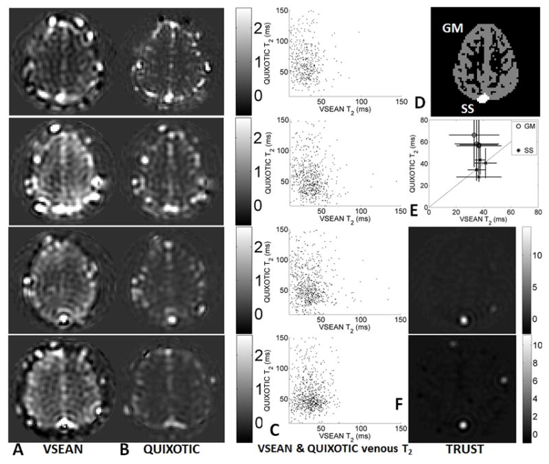
A. VSEAN, B. QUIXOTIC, and F. TRUST images at eTE=20ms, acquired under normoxic conditions on subjects 1–4 (top to bottom, TRUST data only on subjects 3 and 4); C. Scatter plots showing the pixel-wise comparison of T₂’s measured from Gray Matter ROI for each subject; D. representative ROI’s of Gray Matter and Sagittal Sinus used in analysis; E. comparison of means and STD’s of T2 values measured using VSEAN and QUIXOTIC with the unity line shown diagonally, and the STD’s of VSEAN T2 shown horizontally and QUIXOTIC vertically.

For comparison, QUIXOTIC data was collected on subjects 1, 2, 3, and 4, and TRUST data on subject 3 and 4. The imaging parameters were the same as in VSEAN unless noted otherwise. The QUIXOTIC data acquired on subject 1 had initial resolution 48*48 instead of 32*32. Other tagging parameters are listed below.

QUIXOTIC

Two VS preparation modules were used, with v_cut=2cm/s in the slice-select direction. The first one was 722ms before image acquisition, followed by a global inversion pulse 400ms later, and the second VS module was immediately before the imaging excitation pulse (26,27). The second VS module was a VSE/T₂prep module, the flow-weighting gradients were turned on and off under tag and control conditions accordingly, the same eTE’s were used as in VSEAN experiments, 120 acquisitions after 2 dummy scans, scan time 6min 6sec.

TRUST

The thickness of inversion slab was set to 50mm, 25mm above the imaging plane, with TI 1200ms (25). A BIR4-based T₂ preparation module was used with the same eTE’s, TR/TE=8s/26ms, and 36 repetitions were acquired without dummy acquisitions, scan time 4min 48sec.

QUIXOTIC and TRUST images were obtained by subtracting the “tag” and “control” images after averaging. T₂ values were then calculated the same way as in VSEAN. GM and SS ROI analyses were performed on QUIXOTIC data, and SS on TRUST.

Venous T₂ measurements under hypoxia

Subjects 2 and 5 were scanned using VSEAN during normoxia and during a hypoxia challenge. Arterial O₂ saturation levels were monitored by a pulse oximeter on subject’s finger (MRI 3150 Physiological Monitor, Invivo Research) throughout the experiments. During the normoxia scans, normal air (20.9% O₂, rest N₂) was delivered to subjects through a mask. The gas was switched to a hypoxic mixture (12.4% O₂, rest N₂) from a rubber balloon during the hypoxia scans. The hypoxia VSEAN scans started 10–15 min’s after switching the gas when the arterial O₂ saturation level stabilized below 90%. A non-AN scan was performed first, followed by AN scan. The imaging parameters were the same as in other VSEAN scans, except that the repetitions were 96, 4min 48sec each, for subject 5, including 6 “cos” modulated repetitions.

Results

Experiments using a stationary phantom

As shown in Figure 4, the signal from stationary spins was suppressed after “sin” modulated VSE. The residual static signal (“real” component) was neatly separated from the moving signal (“imaginary” component) after projection, which was kept around the noise level. The residual signal in QUIXOTIC (not shown here) after subtraction was well above noise level. However, after increasing the gaps (~6–8ms) after the flow-weighting gradients, the residuals were reduced to similar level as in the VSE experiment after T₂ decay correction. This suggested that the subtraction error observed in the QUIXOTIC experiment could be mainly from eddy current effects. The error due to diffusion attenuation was not observed in QUIXOTIC experiment on this phantom. In comparison, increasing the gaps in the VSE pulse train only improved the residual static tissue signal suppression before projection; and no effect was observed on the “imaginary” component after projection.

FIG. 4.

VSE data collected on a stationary gel phantom (a.u.). A. “cos” modulated, magnitude image; B. “sin” modulated, “real” component; C. “sin” modulated, “imaginary” component. The root mean square (RMS) signal in the “sin” modulated imaginary component is 0.2% of the fully relaxed signal.

Experiments using a rotating phantom

Measured velocity excitation properties of different components in the VSE pulse train are shown in Figure 5. Flow weighting in the imaging sequence alone (Figure 5A) and a VSE module alone (Figure 5B) both gave sinusoidal and cosinusoidal components as expected. A clear sin²-shaped velocity excitation profile was observed in the imaginary component using “sin” modulated VSE and flow-weighting gradients in imaging, matched well with the prediction (Figure 5C) and the excitation response was flat and close to zero at zero velocity as expected.

FIG. 5.

Velocity excitation profile measured in a rotating gel phantom. A. Real and imaginary components with flow weighting in imaging only; B. Real components with only “cos” modulation and only “sin” modulation, the imaginary components of both “cos” and “sin” modulation were close to zero and are not shown here; C. Real and imaginary components with “sin” modulation and flow weighting in imaging, resulting in a sin² dependence for the imaginary component, which closely matched an ideal sin² curve (see text).

Experiments using a flow phantom

A velocity map, VSEAN images, and T₂ maps are shown in Figure 6. The maximal velocity in ROI’s 1, 2, and 3 were 2.1cm/s, −2.1cm/s, and 7.5cm/s, and the averaged velocity in ROI 4 was −0.18cm/s. As shown in Figure 6E and F, the actually measured signal from static spins in ROI 5 was almost completely suppressed by the “sin” modulated VSE pulse train, while the fast, intermediate and slow flows were preserved, and they matched very well with the predicted signal patterns shown in Figure 6B and C, which were calculated from the magnitude image Figure 6A and the predicted velocity excitation profile generated from the velocity map Figure 6D. These also matched well with the velocity excitation profile measured in the rotating phantom experiment. The results of ROI analysis are summarized in Table 1. The T₂ values measured in high SNR ROI’s were similar, however, slightly decreased T₂ values (<10%) were observed in the fast flow ROI while circulating, presumably due to unstable flow there. And the T₂ fitting in ROI 4 was noisy due to low SNR.

Healthy human volunteer experiments under normoxia

Figure 7 shows arterial-and-venous weighted, venous weighted and arterial weighted VSEAN images acquired from subject 1 at different eTE’s, normalized by the averaged brain tissue signal estimated from reference scans and expressed as percentage maps, as well as T₂ maps calculated from each data set. VSEAN, QUIXOTIC and TRUST data at the lowest eTE from subjects 1–4 are shown in Figure 8A, B and F. The representative ROI’s are shown in Figure 8D, the ROI analysis of signal intensities and T₂ values are summarized in Table 2, and also shown in Figure 8E, and a pixel-wise comparison on the GM T₂ values measured by VSEAN and QUIXOTIC for each subject were shown as scatter plots in Figure 8C. For the VSEAN data, the arterial component was weaker than venous component on all scanned volunteers. Given the velocity sensitivity range (v_e=2cm/s) in this study, and the fact that the arterial blood decelerates quickly from relatively high velocities while the venous blood slowly accelerates to moderate velocities, it is possible that less arterial blood distributes within this velocity range than the venous blood; another possibility could be that some of the inverted arterial blood was replaced by fresh blood in this velocity range therefore only a subset of available arterial signal was detected, or a combination of both.

FIG. 7.

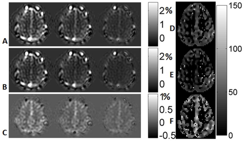
A. non-AN VSEAN images at different eTE’s (arterial and venous, normalized and windowed from −0.5% to 2.5%, see text); B. AN VSEAN images (venous, the display range from −0.5% to 2.5%); C. difference images of A–B, (arterial, −0.5% to 1.1%); D. T₂ map calculated from A (arterial and venous, ms); E. T₂ map calculated from B (venous, ms); F. T₂ map calculated from C (arterial, ms).

As shown in Figure 8, the VSEAN signal was higher than the QUIXOTIC signal, especially on subject 4. In addition to the higher SNR efficiency in theory (Figure 1), another reason could be that QUIXOTIC and VSEAN measured different populations of venous blood: QUIXOTIC assumes that the venous blood is accelerating, thus it detects only the portion that accelerates above v_cut (2cm/s), while VSEAN measures venous blood mainly in the velocity range 0–4 cm/s. So it is possible that the QUIXOTIC sampled only a portion of the venous blood that VSEAN captured.

It is notable that the VSEAN signals (arterial and venous) are related to but not proportional to cerebral blood volumes (CBVs), because these signals are modulated by a sin²-shaped velocity excitation profile. The arterial VSEAN signal may be further reduced by incomplete inversion of the arterial blood pool. Nevertheless, these signals provide rough estimates of the arterial, venous and total CBVs, and they are in the expected range, less than 3% in the brain tissue (Figures 7, 8 and Table 2).

To quantitatively assess if the mean venous T₂ values in SS across subjects are consistent using VSEAN, QUIXOTIC and TRUST, a one-way ANOVA was performed. No significant difference was found (p=0.61, F=0.52, doff=2, total sample size=10, post-hoc power>0.73 using the statistical software package G*power 3.1.3 (46)). However, the T₂ values from GM using QUIXOTIC were higher than all other measurements including QUIXOTIC in SS, a same trend was found when comparing QUIXOTIC in GM and TRUST in SS in ref.(27). A paired t-test was performed on the mean GM venous T₂ values across subjects measured by VSEAN and QUIXOTIC, and showed that T₂ values measured by QUIXOTIC were significantly higher than those by VSEAN (t(3)=7.87, p=0.004, post hoc power>0.78). The higher T₂ values in the GM ROI by QUIXOTIC could be due to CSF contamination from diffusion attenuation, or subtraction error from eddy current effects for the reasons discussed above.

For VSEAN measurement, the T₂ values calculated from the arterial, arterial and venous, venous components followed a descending trend as expected. The mean venous T₂ values measured in the SS were close to those measured in the GM ROI, except in subject 1 where the mean T₂ value in the SS ROI was higher.

The venous T₂ value measured in the GM/whole brain was 35.3±1.6ms (mean±SD) and 37.6±2.8ms in the SS across subjects 1–4 under normal condition. Although the T₂ fitting of the arterial components was noisier than that of the venous components due to lower SNR, higher arterial T₂ values (55.7±9.6ms) were observed with a difference of 20.4ms on the group means, except that on subject 3 where a lower than group mean arterial T₂ value was observed.

The mean oxygenation levels measured in the SS were 67.2±2.5% (n=4) by VSEAN, 66.7±3.9% (n=4) by QUIXOTIC, and 64.0±1.1% (n=2) by TRUST, which are consistent with another study using TRUST (64.8 ±6.3% (n=24) (25)). The mean oxygenation level measured in the GM was 60.5±2.5% (n=4) by VSEAN, which is comparable with literature values: 1) 61.7±5.3% using qBOLD (n=9, GM and WM, calculated using Y_a=100% and OEF=38.3±5.3%) (10); and 2) 62% using PET (n=24, GM, calculated from Y_a=100% and OEF=38%) (47). In contrast, the mean GM oxygenation level measured by QUIXOTIC was76.9±2.8% (n=4), which is significantly higher (t(3)=6.50, p=0.007, post hoc power>0.75) than VSEAN.

Venous T₂ measurements under hypoxia

During the normoxia scans, the arterial O₂ saturation levels were 98% for both subjects 2 and 5; in the hypoxia scans, the saturation levels on subject 2 were between 84–86% during non-AN scan and 82–84% during AN scan; the saturation levels on subject 5 were between 86–88% in both AN and non-AN scans. The average changes of arterial O₂ saturation were 14% for subject 2 and 11% for subject 5.

Abnormal signal variations near the center of the brain were observed in subjects 2 and 5 (images not shown), but the high SNR signals in SS ROI seemed not to be affected, so only the SS ROI was used for both subjects 2 and 5 when comparing the normoxic and hypoxic experimental results.

The results of SS ROI analysis are listed in Table 3. A change of T₂ was detected, corresponding to an oxygenation change. The smaller venous oxygenation change in subject 5 was also reflected in the VSEAN results. The O₂ saturation changes measured by VSEAN (on the venous side) was smaller than that measured by oximeter (on the arterial side), this could be due to increased blood flow during acute hypoxia (48) which reduced the oxygenation change.

Table 3.

T₂ values and oxygenation levels measured under normoxic and hypoxic conditions.

Subject Sex		Normoxia		Hypoxia
	ROI	SS		SS
		T2 (ms)	O2 (%)	T2 (ms)	O2 (%)
2 M	A&V	41.8±5.0	70.9±3.7	29.7±1.8	59.4±2.1
	V	37.8±3.2	67.8±2.8	29.2±2.8	58.7±3.3
5 M	A&V	45.5±5.8	73.5±3.8	38.1±6.9	67.6±5.5
	V	45.7±5.1	73.8±3.2	38.8±6.3	68.3±5.0

On both subjects 2 and 5, decreased VSEAN signals were observed during the hypoxia scans compared to the normoxia scans at the same eTE. This was mainly due to signal decay with lowered T₂ during hypoxia. Another factor that may affect the magnitude of the VSEAN signal is that the blood flow change during hypoxia might shift its velocity distribution, causing a change in the amount of flowing spins under observation. However, a decreased VSEAN signal should not bias the T₂ values, though its accuracy may be affected by decreased SNR.

Discussion

The central features of the proposed VSEAN sequence were successfully demonstrated in phantom and human volunteer experiments, including static tissue suppression, velocity-selective excitation, arterial nulling and T₂ and oxygenation estimation. With a strictly positive sin²-shaped velocity excitation profile, VSEAN technique is immune to signal cancellation from flows in opposite directions. Flow geometry will affect the amplitude of the VSEAN signal, but in theory should not bias the T₂ measurement. However, the flow phantom studies indicated a minor trend of T₂ value lowering when the sample was moving and the VSEAN signal was very low. This may be caused by noise introduced by unstable flows in the phantom, or because the eTE’s (10/30/70ms or 30/50/90ms) used here were not optimal to measure the sample with such long T₂ (~240ms), or flow effects. Fortunately, this effect would be less significant when measuring the blood T₂ (<120ms). Nevertheless, this bias should be investigated more carefully in the future.

The velocity sensitivity of VSE pulse train and the contribution of blood from different sizes of vessels can be adjusted by changing the flow-weighting gradients. Analogous to the consideration of v_cut in VSASL experiment (49), lower v_e will bring the measurement closer to the tissue with improved localization but may cause signal reduction. In this study, the chosen v_e of 2cm/scorresponds to venules/veins of diameters ranging from 100μm to 200μm in human retina (50). However, one would expect the mean velocities in venules/veins of the same size to be lower, as found by other studies on small animals, in the range of 0.8–1.8cm/s (hamster) (51), 0.3–0.5cm/s (cat sartorius muscle) (52). These results from small animals may not be directly applicable to the human brain. However, they suggest that lower v_e may be used in future experiments to optimize the SNR, which depends on the velocity distribution of the venous or arterial population of interest, and also to improve the localization of the VSEAN signal to tissue. The contribution from CSF was found to be negligible since the T₂ values were not biased towards that of CSF. However, lower v_e may generate a stronger signal from CSF, as the velocity of CSF on the surface of the brain is as high as 1.26cm/s in the anterior cranial subarachnoid space (SAS) or 0.28cm/s in the posterior cranial SAS within a cardiac cycle (53).

It is notable that in contrast to the VSASL experiment, there is not enough time between the VSE pulse train and the image acquisition for the blood at various velocities to mix, thus the sin²-shaped velocity excitation profile will largely remain, and higher harmonics (e.g., v=3v_e, 5v_e, …) will also contribute to the total signal (Figure 6). This provides the opportunity to observe the VSEAN signals in large vessels at the same time (Figure 7 & 8). In brain tissue, the contribution from higher harmonics may not be significant due to the relatively narrow velocity distribution range on the venous side.

In order to eliminate the arterial contribution to the venous weighted signal, the nulled arterial blood should occupy the vessels with the velocity range of interest. This requires that at the time of imaging: 1) the leading edge of the inverted arterial bolus decelerates below v_e; and 2) the tail of the bolus has not yet entered the slice of interest. The former depends on the arterial transit time (ATT), i.e., the time for the inverted arterial blood to travel to arterioles or the arterial side of the capillaries, so that TI>ATT; while the latter depends on both the arterial transit time and the temporal width of the inverted arterial bolus, τ, so that TI<ATT+τ. A 20mm gap between the inversion slab and the imaging slab yields an ATT of about 630ms (54). In this study, we estimated an ATT of about 700ms with the 25mm gap used. With an inversion slab thickness of 200mm, τ should be above 800ms, since a typical inversion slab thickness of 100mm yields a τ of 600ms (55), so the TI 1150mm in this study should satisfy both TI>ATT and TI<ATT+τ. However, if the ATT increases significantly such that it exceeds the null point of arterial blood, e.g., under diseased conditions, this could bias the VSEAN measurement towards arterial side. On the other hand, ATT in QUIXOTIC is short and less likely to change under diseased conditions, though it has lower SNR and potential diffusion and eddy current issues as discussed before. Thus, combining these two techniques together may provide a solution in the presence of prolonged ATT, i.e., combining the VS modules from QUIXOTIC for insensitivity to ATT with “cos/sin” modulation and signal projection from VSEAN for venous signal isolation.

In this study, T₂ preparation was used to measure the T₂ values. Multi-echo SE measurement provides higher temporal resolution and efficiency and is less sensitive to fluctuations across TR’s. However, the accuracy of the T₂ measurement may be compromised by artifacts from flow through the multi-echo imaging gradients, even echo refocusing effects (20,56), and wash-out effects across slice-selective refocusing pulses. Nevertheless, because of the higher temporal and SNR efficiency, multi-echo approaches to T₂ measurement are an ongoing subject of study in our laboratory.

It is notable that the measured arterial T₂ values in this study were lower than those measured in big vessels (23), but in good agreement with the trend found in ref. (32,33), that the arterial T₂ decreases as the arterial blood travels to smaller arteries and arterioles or even in capillaries due to the fast water exchange with tissues. As for the venous-weighted signal, when T₂-prep pulses were applied, water traveled downstream in venules where the fast water exchange was less likely to occur, possibly resulting in more reasonable T₂ values. Though lowered hematocrit in small vessels (57,58) is expected to raise the T₂ values (29,59), this was not observed in our experiments or was overwhelmed by the influence of fast water exchange.

The T₂ values measured with BIR4-based VSE/T₂prep module with variable gaps (VG) were lower than those measured using variable numbers (VN) of refocusing pulses (23,25). There may be at least two reasons for this. First, according to the Luz-Meiboom model (60), the apparent T₂ depends on the repetition rate of refocusing pulses in the presence of proton exchange between sites. With the VN method, the refocusing rate is kept constant, while with the VG method the rate decreases. Second, in VN method, spins experience more T_1ρ relaxation and less T₂ decay during the refocusing pulses in ΔeTE, while in the VG method, spins experience pure T₂ decay during ΔeTE. Among the available calibration models from the literature, the one given in ref. (29) used the VG method, and was the most suitable for this study. However, the sequence to acquire the T₂ values in this study was not exactly the same as in ref. (29), and may still result in inaccurate estimate of oxygenation level, as suggested from the arterial T₂-Y measurement in this study. Therefore a calibration curve acquired using the same BIR4-based VSE/T₂prep would be preferred to give a better estimate of oxygenation measured by VSEAN, or a more careful study should be carried out to characterize the behavior of the pulse when the flow signal is very low.

It is also notable that the arterial O₂ saturation levels in GM were lower than one would expect, especially in subject 3. Possible reasons include: 1) lower T₂ due to fast water exchange resulting in lower apparent O₂ saturation levels; 2) actual oxygen loss along the vascular tree might occur earlier in the arterioles (61,62), e.g., the maximum oxygen saturation in arterioles could be as low as 89.6±6.0% (51), or the measurement was biased toward the capillary side rather than to the arteriole side when the post-labeling delay was long; 3) low SNR; and 4) possible bias to the O₂ saturation introduced by errors in the T₂-Y calibration curve.

The detection and separation of venous and arterial signal in the GM and SS was demonstrated in this study. As noted in Figure 8, the VSEAN technique can be applied on other vessels or tissues, e.g., the vessels on the scalp to monitor the metabolic rate of the scalp, or the vessels of the neck to simultaneously measure the arterial and venous oxygenation, and thereby the metabolic rate of the whole brain.

Currently, the VSEAN technique is limited to single-slice acquisition due to the single nulling point of arterial blood. To increase coverage, this technique is amenable to 3D acquisition.

Conclusions

The new VSEAN technique was demonstrated to efficiently isolate flow signals from static signals in phantoms, and venous-weighted signals from surrounding static tissue in both small and big veins in human volunteers. T₂ and oxygenation mapping of both venous and arterial blood in the brain was shown, as well as successful detection of the change of T₂ and oxygenation during a hypoxia challenge. Compared to the QUIXOTIC technique, the SNR, temporal efficiency and insensitivity to slow motion are improved, and contamination from diffusion attenuation is eliminated.

References

- 1.Astrup J, Siesjo BK, Symon L. Thresholds in cerebral ischemia - the ischemic penumbra. Stroke. 1981;12(6):723–725. doi: 10.1161/01.str.12.6.723. [DOI] [PubMed] [Google Scholar]
- 2.Baron JC, Bousser MG, Rey A, Guillard A, Comar D, Castaigne P. Reversal of focal “misery-perfusion syndrome” by extra-intracranial arterial bypass in hemodynamic cerebral ischemia. A case study with 15O positron emission tomography. Stroke. 1981;12(4):454–459. doi: 10.1161/01.str.12.4.454. [DOI] [PubMed] [Google Scholar]
- 3.Baron JC. Mapping the ischaemic penumbra with PET: implications for acute stroke treatment. Cerebrovasc Dis. 1999;9(4):193–201. doi: 10.1159/000015955. [DOI] [PubMed] [Google Scholar]
- 4.Guadagno JV, Warburton EA, Aigbirhio FI, Smielewski P, Fryer TD, Harding S, Price CJ, Gillard JH, Carpenter TA, Baron J-C. Does the Acute Diffusion-Weighted Imaging Lesion Represent Penumbra as Well as Core? A Combined Quantitative PET/MRI Voxel-Based Study. J Cereb Blood Flow Metab. 2004:1249–1254. doi: 10.1097/01.WCB.0000141557.32867.6B. [DOI] [PubMed] [Google Scholar]
- 5.Sobesky J, Weber OZ, Lehnhardt FG, Hesselmann V, Neveling M, Jacobs A, Heiss WD. Does the Mismatch Match the Penumbra?: Magnetic Resonance Imaging and Positron Emission Tomography in Early Ischemic Stroke. Stroke. 2005;36(5):980–985. doi: 10.1161/01.STR.0000160751.79241.a3. [DOI] [PubMed] [Google Scholar]
- 6.Abate MG, Trivedi M, Fryer TD, Smielewski P, Chatfield DA, Williams GB, Aigbirhio F, Carpenter TA, Pickard JD, Menon DK, Coles JP. Early Derangements in Oxygen and Glucose Metabolism Following Head Injury: The Ischemic Penumbra and Pathophysiological Heterogeneity. Neurocrit Care. 2008;9(3):319–325. doi: 10.1007/s12028-008-9119-2. [DOI] [PubMed] [Google Scholar]
- 7.Heiss WD. Identifying Thresholds for Penumbra and Irreversible Tissue Damage. Stroke. 2004;35(11_suppl_1):2671–2674. doi: 10.1161/01.STR.0000143329.81997.8a. [DOI] [PubMed] [Google Scholar]
- 8.Ogawa S, Lee T-M. Magnetic resonance imaging of blood vessels at high fields: in vivo and in vitro measurements and image simulation. Magn Reson Med. 1990;16:9–18. doi: 10.1002/mrm.1910160103. [DOI] [PubMed] [Google Scholar]
- 9.Davis TL, Kwong KK, Weisskoff RM, Rosen BR. Calibrated functional MRI: mapping the dynamics of oxidative metabolism. Proc Natl Acad Sci USA. 1998;95:1834–1839. doi: 10.1073/pnas.95.4.1834. [DOI] [PMC free article] [PubMed] [Google Scholar]
- 10.He X, Yablonskiy DA. Quantitative BOLD: Mapping of human cerebral deoxygenated blood volume and oxygen extraction fraction: Default state. Magn Reson Med. 2007;57(1):115–126. doi: 10.1002/mrm.21108. [DOI] [PMC free article] [PubMed] [Google Scholar]
- 11.Yablonskiy DA, Haacke EM. Theory of Nmr Signal Behavior in Magnetically Inhomogeneous Tissues - the Static Dephasing Regime. Magn Reson Med. 1994;32(6):749–763. doi: 10.1002/mrm.1910320610. [DOI] [PubMed] [Google Scholar]
- 12.Christen T, Lemasson B, Pannetier N, Farion R, Segebarth C, Remy C, Barbier EL. Evaluation of a quantitative blood oxygenation level-dependent (qBOLD) approach to map local blood oxygen saturation. NMR Biomed. 2011;24(4):393–403. doi: 10.1002/nbm.1603. [DOI] [PubMed] [Google Scholar]
- 13.Jain V, Langham MC, Wehrli FW. MRI estimation of global brain oxygen consumption rate. J Cereb Blood Flow Metab. 2010;30(9):1598–1607. doi: 10.1038/jcbfm.2010.49. [DOI] [PMC free article] [PubMed] [Google Scholar]
- 14.Fernández-Seara MA, Techawiboonwong A, Detre JA, Wehrli FW. MR susceptometry for measuring global brain oxygen extraction. Magn Reson Med. 2006;55(5):967–973. doi: 10.1002/mrm.20892. [DOI] [PubMed] [Google Scholar]
- 15.Haacke EM, Lai S, Reichenbach JR, Kuppusamy K, Hoogenraad FGC, Takeichi H, Lin WL. In vivo measurement of blood oxygen saturation using magnetic resonance imaging: A direct validation of the blood oxygen level-dependent concept in functional brain imaging. Hum Brain Mapp. 1997;5(5):341–346. doi: 10.1002/(SICI)1097-0193(1997)5:5<341::AID-HBM2>3.0.CO;2-3. [DOI] [PubMed] [Google Scholar]
- 16.Lu HZ, van Zijl PCM. Experimental measurement of extravascular parenchymal BOLD effects and tissue oxygen extraction fractions using multi-echo VASO fMRI at 1.5 and 3.0 T. Magn Reson Med. 2005;53(4):808–816. doi: 10.1002/mrm.20379. [DOI] [PubMed] [Google Scholar]
- 17.An HY, Lin WL. Quantitative measurements of cerebral blood oxygen saturation using magnetic resonance imaging. J Cereb Blood Flow Metab. 2000;20(8):1225–1236. doi: 10.1097/00004647-200008000-00008. [DOI] [PMC free article] [PubMed] [Google Scholar]
- 18.Foltz WD, Merchant N, Downar R, Stainsby TA, Wright GA. Coronary venous oximetry using MRI. Magn Reson Med. 1999;42(5):837–848. doi: 10.1002/(sici)1522-2594(199911)42:5<837::aid-mrm3>3.0.co;2-8. [DOI] [PubMed] [Google Scholar]
- 19.Oja JM, Gillen JS, Kauppinen RA, Kraut M, van Zijl PC. Determination of oxygen extraction ratios by magnetic resonance imaging. J Cereb Blood Flow Metab. 1999;19(12):1289–1295. doi: 10.1097/00004647-199912000-00001. [DOI] [PubMed] [Google Scholar]
- 20.Golay X, Silvennoinen MJ, Zhou J, Clingman CS, Kauppinen RA, Pekar JJ, van Zij PC. Measurement of tissue oxygen extraction ratios from venous blood T(2): increased precision and validation of principle. Magn Reson Med. 2001;46(2):282–291. doi: 10.1002/mrm.1189. [DOI] [PubMed] [Google Scholar]
- 21.Wright GA, Hu BS, Macovski A. Estimating Oxygen Saturation of Blood In vivo with MR Imaging at 1.5T. J Magn Reson Im. 1991;1(3):275–283. doi: 10.1002/jmri.1880010303. [DOI] [PubMed] [Google Scholar]
- 22.Chien D, Levin DL, Anderson CM. MR gradient echo imaging of intravascular blood oxygenation: T2* determination in the presence of flow. Magn Reson Med. 1994;32(4):540–545. doi: 10.1002/mrm.1910320419. [DOI] [PubMed] [Google Scholar]
- 23.Lee T, Stainsby JA, Hong J, Han E, Brittain J, Wright GA. Blood Relaxation Properties at 3T --Effects of Blood Oxygen Saturation. Proceedings of the 11th Annual Meeting of ISMRM; Toronto, Ontario, Canada. 2003. p. 131. [Google Scholar]
- 24.Yablonskiy DA. Quantitation of intrinsic magnetic susceptibility-related effects in a tissue matrix. Phantom study Magn Reson Med. 1998;39(3):417–428. doi: 10.1002/mrm.1910390312. [DOI] [PubMed] [Google Scholar]
- 25.Lu HZ, Ge YL. Quantitative evaluation of oxygenation in venous vessels using T2-Relaxation-Under-Spin-Tagging MRI. Magn Reson Med. 2008;60(2):357–363. doi: 10.1002/mrm.21627. [DOI] [PMC free article] [PubMed] [Google Scholar]
- 26.Bolar DS, Rosen BR, Sorensen AG, Adalsteinsson E. QUantitative Imaging of eXtraction of Oxygen and TIssue Consumption (QUIXOTIC) using velocity selective spin labeling. Proceedings of the 17th Annual Meeting of ISMRM; Honolulu, Hawai’i, USA. 2009. p. 628. [DOI] [PMC free article] [PubMed] [Google Scholar]
- 27.Bolar DS. PhD Thesis. Cambridge: Massachusetts Institute of Technology; 2010. Magnetic resonance imaging of the cerebral metabolic rate of oxygen (CMRO2) [Google Scholar]
- 28.Guo J, Wong EC. Imaging of Oxygen Extraction Fraction Using Velocity Selective Excitation with Arterial Nulling (VSEAN). Proceedings of the 18th Annual Meeting of ISMRM; Stockholm, Sweden. 2010. p. 4057. [Google Scholar]
- 29.Zhao JM, Clingman CS, Närväinen MJ, Kauppinen RA, van Zijl PCM. Oxygenation and hematocrit dependence of transverse relaxation rates of blood at 3T. Magn Reson Med. 2007;58(3):592–597. doi: 10.1002/mrm.21342. [DOI] [PubMed] [Google Scholar]
- 30.Chen JJ, Pike GB. Human whole blood T2 relaxometry at 3 Tesla. Magn Reson Med. 2009;61(2):249–254. doi: 10.1002/mrm.21858. [DOI] [PubMed] [Google Scholar]
- 31.Stefanovic B, Pike GB. Human whole-blood relaxometry at 1.5T: Assessment of diffusion and exchange models. Magn Reson Med. 2004;52(4):716–723. doi: 10.1002/mrm.20218. [DOI] [PubMed] [Google Scholar]
- 32.Wells JA, Lythgoe MF, Choy M, Gadian DG, Ordidge RJ, Thomas DL. Characterizing the origin of the arterial spin labelling signal in MRI using a multiecho acquisition approach. Journal of Cerebral Blood Flow; Metabolism. 2009;29(11):1836–1845. doi: 10.1038/jcbfm.2009.99. [DOI] [PubMed] [Google Scholar]
- 33.Liu P, Uh J, Lu H. Determination of spin compartment in arterial spin labeling MRI. Magn Reson Med. 2011;65(1):120–127. doi: 10.1002/mrm.22601. [DOI] [PMC free article] [PubMed] [Google Scholar]
- 34.Wong EC, Guo J. BIR-4 based B1 and B0 insensitive velocity selective pulse trains. Proceedings of the 18th Annual Meeting of ISMRM; Stockholm, Sweden. 2010. p. 2853. [Google Scholar]
- 35.Wong EC, Cronin M, Wu W-C, Inglis B, Frank LR, Liu TT. Velocity Selective Arterial Spin Labeling. Magn Reson Med. 2006;55:1334–1341. doi: 10.1002/mrm.20906. [DOI] [PubMed] [Google Scholar]
- 36.Norris DG, Schwartzbauer C. Velocity Selective Radiofrequency Pulse Trains. J Magn Reson. 1999;137:231–236. doi: 10.1006/jmre.1998.1690. [DOI] [PubMed] [Google Scholar]
- 37.Garwood M, DelaBarre L. The return of the frequency sweep: designing adiabatic pulses for contemporary NMR. J Magn Reson. 2001;153(2):155–177. doi: 10.1006/jmre.2001.2340. [DOI] [PubMed] [Google Scholar]
- 38.Silver MS, Joseph RI, Hoult DI. Selective spin inversion in nuclear magnetic resonance and coherent optics through an exact solution of the Bloch-Riccati equation. Phys Rev A. 1985;31:2753–2755. doi: 10.1103/physreva.31.2753. [DOI] [PubMed] [Google Scholar]
- 39.Wong EC, Buxton RB, Frank LR. Implementation of quantitative perfusion imaging techniques for functional brain mapping using pulsed arterial spin labeling. NMR in Biomed. 1997;10:237–249. doi: 10.1002/(sici)1099-1492(199706/08)10:4/5<237::aid-nbm475>3.0.co;2-x. [DOI] [PubMed] [Google Scholar]
- 40.Edelman RR, Siewert B, Darby DG, Thangaraj V, Nobre AC, Mesulam MM, Warach S. Qualitative mapping of cerebral blood flow and functional localization with echo-planar MR imaging and signal targeting with alternating radio frequency (STAR) sequences: applications to MR angiography. Radiology. 1994;192:513–520. doi: 10.1148/radiology.192.2.8029425. [DOI] [PubMed] [Google Scholar]
- 41.Kwong KK, Belliveau JW, Chesler DA, Goldberg IE, Weisskoff RM, Poncelet BP, Kennedy DN, Hoppel BE, Cohen MS, Turner R, Cheng H-M, Brady TJ, Rosen BR. Dynamic magnetic resonance imaging of human brain activity during primary sensory stimulation. Proc Natl Acad Sci USA. 1992;89:5675–5679. doi: 10.1073/pnas.89.12.5675. [DOI] [PMC free article] [PubMed] [Google Scholar]
- 42.Kim S-G. Quantification of regional cerebral blood flow change by flow-sensitive alternating inversion recovery (FAIR) technique: application to functional mapping. Magn Reson Med. 1995;34:293–301. doi: 10.1002/mrm.1910340303. [DOI] [PubMed] [Google Scholar]
- 43.Nezafat R, Ouwerkerk R, Derbyshire AJ, Stuber M, McVeigh ER. Spectrally selective B1-insensitive T2 magnetization preparation sequence. Magn Reson Med. 2009;61(6):1326–1335. doi: 10.1002/mrm.21742. [DOI] [PubMed] [Google Scholar]
- 44.de Graaf RA, Rothman DL, Behar KL. Adiabatic RARE imaging. NMR Biomed. 2003;16(1):29–35. doi: 10.1002/nbm.811. [DOI] [PubMed] [Google Scholar]
- 45.Lu H, Clingman C, Golay X, van Zijl PCM. Determining the longitudinal relaxation time (T1) of blood at 3.0 Tesla. Magn Reson Med. 2004;52(3):679–682. doi: 10.1002/mrm.20178. [DOI] [PubMed] [Google Scholar]
- 46.Erdfelder E, Faul F, Buchner A, Lang AG. Statistical power analyses using G*Power 3.1: Tests for correlation and regression analyses. Behav Res Methods. 2009;41(4):1149–1160. doi: 10.3758/BRM.41.4.1149. [DOI] [PubMed] [Google Scholar]
- 47.Leenders KL, Perani D, Lammertsma AA, Heather JD, Buckingham P, Healy MJR, Gibbs JM, Wise RJS, Hatazawa J, Herold S, Beaney RP, Brooks DJ, Spinks T, Rhodes C, Frackowiak RSJ, Jones T. Cerebral Blood-Flow, Blood-Volume and Oxygen Utilization - Normal Values and Effect of Age. Brain. 1990;113:27–47. doi: 10.1093/brain/113.1.27. [DOI] [PubMed] [Google Scholar]
- 48.Dubowitz DJ, Dyer EA, Theilmann RJ, Buxton RB, Hopkins SR. Early brain swelling in acute hypoxia. J Appl Physiol. 2009;107(1):244–252. doi: 10.1152/japplphysiol.90349.2008. [DOI] [PMC free article] [PubMed] [Google Scholar]
- 49.Wu WC, Wong EC. Intravascular effect in velocity-selective arterial spin labeling: the choice of inflow time and cutoff velocity. Neuroimage. 2006;32(1):122–128. doi: 10.1016/j.neuroimage.2006.03.001. [DOI] [PubMed] [Google Scholar]
- 50.Riva CE, Grunwald JE, Sinclair SH, Petrig BL. Blood velocity and volumetric flow rate in human retinal vessels. Invest Ophthalmol Vis Sci. 1985;26(8):1124–1132. [PubMed] [Google Scholar]
- 51.Alves de Mesquita J, Jr, Bouskela E, Wajnberg E, Lopes de Melo P. Improved instrumentation for blood flow velocity measurements in the microcirculation of small animals. Rev Sci Instrum. 2007;78(2):024303. doi: 10.1063/1.2668504. [DOI] [PubMed] [Google Scholar]
- 52.House SD, Johnson PC. Diameter and Blood-Flow of Skeletal-Muscle Venules during Local Flow Regulation. Am J Physiol. 1986;250(5):H828–H837. doi: 10.1152/ajpheart.1986.250.5.H828. [DOI] [PubMed] [Google Scholar]
- 53.Kurtcuoglu V, Gupta S, Soellinger M, Grzybowski DM, Boesiger P, Biddiscombe J, Poulikakos D. Cerebrospinal fluid dynamics in the human cranial subarachnoid space: an overlooked mediator of cerebral disease. I. Computational model. Journal of the Royal Society Interface. 2010;7(49):1195–1204. doi: 10.1098/rsif.2010.0033. [DOI] [PMC free article] [PubMed] [Google Scholar]
- 54.Qiu M, Paul Maguire R, Arora J, Planeta-Wilson B, Weinzimmer D, Wang J, Wang Y, Kim H, Rajeevan N, Huang Y, Carson RE, Constable RT. Arterial transit time effects in pulsed arterial spin labeling CBF mapping: insight from a PET and MR study in normal human subjects. Magn Reson Med. 2010;63(2):374–384. doi: 10.1002/mrm.22218. [DOI] [PMC free article] [PubMed] [Google Scholar]
- 55.Wong EC, Buxton RB, Frank LR. Quantitative imaging of perfusion using a single subtraction (QUIPSS and QUIPSS II) Magn Reson Med. 1998;39:702–708. doi: 10.1002/mrm.1910390506. [DOI] [PubMed] [Google Scholar]
- 56.Kucharczyk W, Brant-Zawadzki M, Lemme-Plaghos L, Uske A, Kjos B, Feinberg DA, Norman D. MR technology: effect of even-echo rephasing on calculated T2 values and T2 images. Radiology. 1985;157(1):95–101. doi: 10.1148/radiology.157.1.4034984. [DOI] [PubMed] [Google Scholar]
- 57.Fahraeus R. The suspension stability of the blood. Physiol Rev. 1929;9(2):241–274. [Google Scholar]
- 58.Levin VA, Gilboe DD. Blood Volume and Hematocrit Relationships in Isolated Perfused Dog Brain. Neurology. 1969;19(3):317. doi: 10.1161/01.str.1.4.270. [DOI] [PubMed] [Google Scholar]
- 59.Hayman LA, Ford JJ, Taber KH, Saleem A, Round ME, Bryan RN. T2 Effect of Hemoglobin Concentration - Assessment with Invitro Mr Spectroscopy. Radiology. 1988;168(2):489–491. doi: 10.1148/radiology.168.2.3393669. [DOI] [PubMed] [Google Scholar]
- 60.Luz Z, Meiboom S. Nuclear Magnetic Resonance Study of Protolysis of Trimethylammonium Ion in Aqueous Solution - Order of Reaction with Respect to Solvent. J Chem Phys. 1963;39(2):366. [Google Scholar]
- 61.Popel AS, Pittman RN, Ellsworth ML. Rate of Oxygen Loss from Arterioles Is an Order of Magnitude Higher Than Expected. Am J Physiol. 1989;256(3):H921–H924. doi: 10.1152/ajpheart.1989.256.3.H921. [DOI] [PubMed] [Google Scholar]
- 62.Kobayashi H, Takizawa N. Imaging of oxygen transfer among microvessels of rat cremaster muscle. Circulation. 2002;105(14):1713–1719. doi: 10.1161/01.cir.0000013783.63773.8f. [DOI] [PubMed] [Google Scholar]