Statistical Significance of Optical Map Alignments

Abstract

The Optical Mapping System constructs ordered restriction maps spanning entire genomes through the assembly and analysis of large datasets comprising individually analyzed genomic DNA molecules. Such restriction maps uniquely reveal mammalian genome structure and variation, but also raise computational and statistical questions beyond those that have been solved in the analysis of smaller, microbial genomes. We address the problem of how to filter maps that align poorly to a reference genome. We obtain map-specific thresholds that control errors and improve iterative assembly. We also show how an optimal self-alignment score provides an accurate approximation to the probability of alignment, which is useful in applications seeking to identify structural genomic abnormalities.

1. Introduction

A genome-wide restriction map identifies cognate sites (4–8 bp) at which restriction endonucleases selectively recognize and cleave DNA. Consequently, comparison of a reference and a test genome restriction map comprehensively reveals a rich compendium of genomic differences: single nucleotide polymorphisms (SNPs) that simply create and remove restriction sites, and structural variants comprising insertions, deletions, inversions, translocations, and gross rearrangements that alter the size, or order of restriction fragments. Such analysis is now a proven means for discovering and characterizing the full range of structural variation in human populations (Teague et al., 2010).

The advantages offered by restriction maps for genome analysis are realized by the Optical Mapping System (OM) because it develops and analyzes datasets of individually mapped DNA molecules (Schwartz et al., 1993; Dimalanta et al., 2004; Teague et al., 2010). (A restriction map constructed from a single DNA molecule is called an “Rmap.”) Briefly, large genomic DNA molecules (≈0.5 Mb) are restriction digested after microfluidic deposition onto positively charged glass surfaces. The microfluidic device uses a combination of fluid flow and interaction with a charged surface to unravel and straighten normally coiled DNA molecules. Because deposited molecules are under tension, like a stretched rubber band, restriction cleavage triggers newly formed molecule ends to relax, producing visible gaps and creating strings of discrete DNA fragments that are imaged by automated fluorescence microscopy after staining with a fluorochrome dye. An Rmap acts like a barcode that assigns genomic location to the DNA molecule. Responsive to the unique noise characteristics of OM measurements, computational analysis assembles putative overlapping Rmaps from the many thousands of analyzed molecules into a genome-wide restriction map in ways that closely parallel assembly of shotgun sequence reads. Early in the development of OM, microbial genomes were primarily analyzed as approachable model systems for learning more about the challenges of dealing with larger, more complex genomes. Accordingly, advances in OM have enabled insightful analysis of human (Teague et al., 2010; Kidd et al., 2008; Antonacci et al., 2010) and plant genomes (Zhou et al., 2007; Schnable et al., 2009; Zhou et al., 2009).

Whether or not, and where a given Rmap overlaps another restriction map presents a fundamental inference problem in OM. We are interested in the centrally important question of how to align an Rmap to the genome-wide map created in silico by cleaving a reference genome. In the current state of the art, each possible alignment is scored in a way that rewards matches and penalizes discrepancies, and dynamic programming identifies the optimal alignment (Huang and Waterman, 1992; Valouev et al., 2006). Rmaps having relatively low scores do not align with sufficient fidelity to be useful in subsequent computations, and these must be carefully filtered in a way that recognizes the pattern of variation in the optimal scores. Simple thresholding schemes are inefficient because statistical properties of the optimal score depend on characteristics of the Rmaps being aligned. We investigate this phenomenon and develop computationally efficient Rmap-specific thresholds for identifying non-spurious alignments. We show how properties of genomic assemblies are improved when Rmaps are filtered via Rmap-specific thresholds as opposed to other available methods.

Assembly is the computational process in which the Rmaps become positioned relative to each other, organized at the genomic scale, and summarized by a consensus map. For relatively small genomes, the Gentig algorithm produces de novo assemblies without requiring an initial estimate of the genome-wide restriction map (Anantharaman et al., 1999). This direct approach is not computationally feasible for large (e.g., mammalian-sized) genomes, although de novo genome assembly was accomplished indirectly using a divide an conquer scheme (Zhou et al., 2007, 2009). Alternatively, assemblies are guided by an in silico derived reference map, wherein Gentig is applied locally to relatively small Rmap sets aligning in small regions, and then the local assemblies are stitched together. In iterative assembly, the resulting consensus map is used to guide a subsequent round of alignment, local assembly, and global assembly, and then the whole exercise is repeated until convergence (see Appendix 5.2) (Teague et al., 2010). The decision of whether or not an Rmap aligns to the current consensus map is a key computational element that is called many thousands of times during iterative assembly. The precise rule for declaring alignment significance has an effect on genome assembly and any derived inferences about polymorphism or structural variation.

The optical mapping system was designed and developed to comprehensively reveal human and cancer structural variation: structural variation describes those genomic polymorphisms and mutations ≥1 kb (Scherer et al., 2007). The main strategy for such identification is to assemble the Rmaps and then to detect aberrations by a screen of the assembly against the reference genome (Teague et al., 2010). The detection of copy number variants is a special case that is possible without assembly and thus has some advantages (Sarkar, 2006). Briefly, a copy number gain is indicated if an abnormally large number of Rmaps align at a given locus, while a loss is indicated when too few Rmaps align. Because very long Rmaps (≈0.5 Mb) are tallied in place of probes or short sequence reads, findings are complementary to traditional copy number variant (CNV) analysis (Sebat et al., 2004). There is a statistical bottleneck created by this assembly-free strategy, however, because even in the absence of copy number variation there is variation across the genome in the probability of alignment. As a result, the successfully aligned Rmaps represent a non-uniform thinning of the originals, and a baseline against which copy number variants may be measured is similarly non-uniform. A solution is possible via normalization if we can compute the probability of alignment for each Rmap. We show how a certain self-alignment score provides a fast approximation to the probability of alignment, thus facilitating a normalization of optical map coverage.

Our methods are developed and tested on Rmaps from GM07535, a normal human lymphoblastoid cell line, one of the first applications of OM to the human genome (Lim, 2004). The dataset consists of 206,796 Rmaps, the subset exceeding 0.3 Mb from a larger panel. The Rmaps were aligned against an in silico reference map derived from NCBI Build 35 of the human genome sequence, with sequence gaps replaced by their estimated lengths, and utilizing ungapped global alignment. For validation, we use an independent dataset of 416, 284 Rmaps obtained from a complete hydatidiform mole (CHM), artificially created to be homozygous (Teague et al., 2010). Additionally, we evaluate methods using 50,000 Rmaps simulated from the human reference (Appendix 5.3 gives details of the generative model).

2. Methods

2.1. Map significance

Denote an Rmap by and the in silico reference map by . These record sites of enzyme recognition in the single molecule and the reference genome, respectively. Among all possible alignments of to , allow that an optimal one has maximal score S = S(). We view as arising from by some stochastic mechanism that depends on technical aspects of OM and also biological differences between the sampled genome and the reference. If the signal is sufficiently degraded, then even the optimal alignment is probably incorrect, and using it in assembly, for example, would unduly inflate errors. The problem is to decide whether or not the optimal alignment score S is statistically significant in some sense. This requires a reference distribution for S under a suitable null hypothesis.

Our approach avoids specifying a probability model for the generation of Rmaps. An accurate model might need to be overly complex, while misspecifying the model could lead to additional errors. Instead, we calibrate S() by fixing the Rmap through conditioning and by exploiting statistical features of the genome. Formally, we treat both and as realizations of random objects and , and the null hypothesis H₀ on test is that and are independent. Independence means that knowing one object is of no use in predicting the other. This holds when does not originate from , but also effectively reflects the situation where noise in generating has fully degraded any attributes of . Under H₀, any alignment of to is spurious, and so we call S() (or a realization thereof) a best spurious score.

We make the nonparametric assumption on that it is the concatenation of a set F() of fragments, with fragment sizes that are independent and identically distributed (i.i.d.) random variables. This is weaker, for example, than assuming fragment sizes are i.i.d. exponentially distributed variables, as would be the case in a homogeneous Poisson-process model for (Valouev et al., 2006). 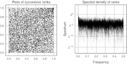A look at empirical fragment sizes in the build 35 supports this treatment (Fig. 1). Rather than adopt a specific fragment model, we instead condition on the set of observed fragment sizes F() in calibrating an alignment. We say that the optimal alignment of to is statistically significant at level α if the optimal score S() exceeds the threshold c_α defined so that the conditional probability

FIG. 1.

Lack of auto-correlation in in silico fragment lengths induced by the SwaI enzyme in build 35 of the human reference genome (chromosome 1). Fragments are ranked by size and then successive pairs of ranks are plotted (left). The uniform scatter is consistent with lack of first-order autocorrelation of fragment sizes. Lack of structure in the spectral density of the ranks is another view consistent with the independence assumption (right). Results from other chromosomes are similar and not shown. The absence of substantial dependence justifies calibration by fragment permutation.

The assumptions taken are precisely those justifying permutation analysis to calibrate S (Cox and Hinkley, 1979). Indeed, permutation is often used in related areas of sequence alignment (Mitrophanov and Borodovsky, 2006). In the absence of computational restrictions, significance could be assessed by generating genomes via random shuffling of fragments, with computed in each case. The (1-α) quantile of the resulting empirical distribution approximates c_α, which is both Rmap- specific and dependent on general features of the genome through F(). The permutation strategy preserves characteristics of the reference that affect the spurious score distribution, namely the number and lengths of fragments. Permuting the order of fragments is also reasonable given the additive nature of score functions, which reward matches in order. A small adjustment to the strategy is suggested by the finding that fragment-size distributions fluctuate among chromosomes; thus the shuffling can be restricted to re-arrange fragments separately on different chromosomes. A larger problem, however, is computational. The strategy seems to require that every Rmap have its optimal alignment score computed on a large number of randomized genomes, which would be prohibitive in routine applications of OM. We introduce two standardized optimal alignment scores that avoid this requirement.

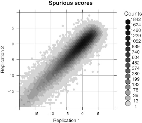
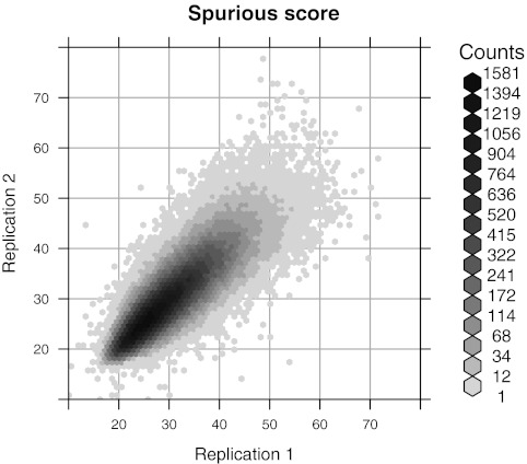
Our computational experiments utilize two scoring functions: a custom score implemented in the SOMA software package (Kohn, 2003), and a likelihood-ratio (LR) score (see Appendix 5.1) (Valouev et al., 2006). Figure 2 exposes the strong dependence of the best spurious SOMA score on (a similar pattern is seen in Fig. 3 with the LR score). Two random permutations of the build 35 were used to produce two optimal scores for each . The correlation between the scores is strong and suggests a decomposition

(1)

FIG. 2.

Dependence of spurious scores on Rmap. For each Rmap, the optimal scores for ungapped global alignment against two independent permutations of the reference are plotted against each other. The scores are highly correlated, indicating a significant Rmap-specific component in the distribution of the best spurious score. The two-dimensional (2-D) histogram uses hexagonal binning (Carr et al., 1987).

FIG. 3.

Likelihood ratio (LR) scores for ungapped global alignment (Valouev et al., 2006). Optimal scores for GM07535 Rmaps aligned against two independent permutations of the in silico reference are plotted against each other.

under H₀, where μ() and σ are the Rmap-specific mean and standard deviation, and is a mean zero, unit variance deviation. Our approach is to standardize by subtracting an estimated mean and scaling by an estimated standard deviation, in order to approximate . One difficulty is in deriving computationally efficient estimates, in place of the obvious estimates obtained by many permutations and re-alignments. For both standardized statistics we treat as a linear function of , namely, . 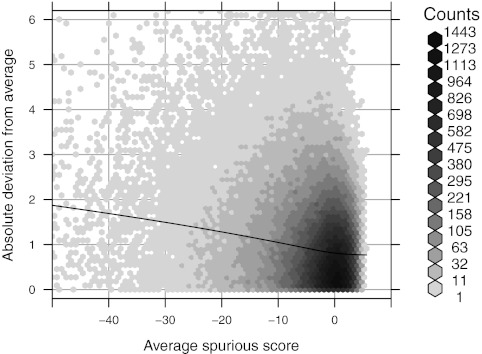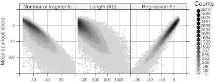This is justified both from Figure 2 and additional numerical experiments (Fig. 4), and allows estimation by fitting a generalized least squares model.

FIG. 4.

Variance of errors. The x-axis encodes the expected best spurious score, , as estimated by the average best spurious score against four permutations of . On the y-axis are absolute deviations from this average of scores against a fifth permutation. The LOESS smooth suggests that the standard deviation of the errors is a linear function of the average spurious score.

Direct approach: Using a relatively small number of permuted reference genomes align to each and construct

Then estimate the scale parameter using alignments of all Rmaps against an additional genomic permutation , and form the standardized statistic (ignoring the constant τ)

Regression approach: Approximate by a linear function of the number of fragments and the base-pair length, with coefficients estimated in a genome-wide multiple linear regression of on the two size predictors (Fig. 5). The model directly incorporates the variance structure, and is estimated using generalized least squares, yielding the standardized statistic

FIG. 5.

Parametric models for , the expected best spurious score. The average of four best spurious scores for each Rmap is plotted against the number of fragments N, the length L, and the fitted values from a linear model with terms N, L, and their product NL. The multiple regression model explains more of the variability and also suggests a more symmetric distribution of the errors.

A further difficulty is in finding a suitable reference distribution for either standardized optimal alignment score. Since standardization has removed the dominant Rmap effects, we can use the empirical distribution of standardized scores computed across all Rmaps on a single genome shuffling. (This step makes the inclusion of τ in the standardized statistics redundant.)

A modified-constant filtering procedure has been useful in lab work. It requires at least n aligned fragments and that the SOMA score S > s. This addresses the need to retain only highly scoring Rmaps, and to accommodate Rmap length characteristics, but it is difficult to tune (no error rates are targeted) and it entails dependence on the alignment itself rather than the Rmap. We compare our proposed thresholding schemes to this modified-constant method for (s = 4.5,n = 10) and (s = 2.75,n = 10).

2.2. Alignment probability

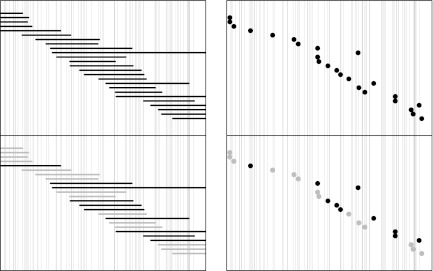
Even for Rmaps derived from a normal genome, significant alignments are not distributed uniformly along the genome, owing to fluctuations in the local characteristics of the normal restriction map. Figure 6 illustrates the non-uniform alignment process. Knowing the null probability that an Rmap will align is necessary to normalize coverage in order to call significant copy number variants in a test genome. To address this problem we consider the logistic approximation

(2)

FIG. 6.

Schematic representation of “thinning” in Rmap alignments. The horizontal axis represents the underlying genome, with vertical lines indicating restriction sites. (Left) Rmaps are represented as intervals. (Right) They are viewed as point events represented by the midpoint of the Rmaps. (Top) The top panel in both plots represent the true shotgun random sample of Rmaps that originated from this region. Actual Rmaps obtained by image processing will have noise, including sizing errors, missing cuts and false cuts, so not all these Rmaps will be successfully aligned. Further, the chance of being aligned may depend on the location of the Rmap; for example, Rmaps with fewer fragments (from regions with fewer recognition sites) may be less likely to align than Rmaps of similar length with more fragments. (Bottom) In the bottom panels, which represent the results of alignment, unaligned Rmaps are indicated in gray. Since the probability of being successfully aligned depends on the origin, the locations of aligned Rmaps, which is what we actually observe, are no longer uniformly distributed.

where α and β are fitted parameters and is the optimal alignment score obtained in aligning an Rmap to itself.

Being the perfect match score, the self-alignment score is a natural measure of information contained in the Rmap. Not only is it higher for Rmaps with more fragments, but it is also affected by the lengths of the component fragments (score functions reward matches involving longer fragments because they are rarer). We expect Rmaps with lower information content to be less likely to align, and we see later that the logistic model above is indeed useful in predicting alignment probability. The self-alignment score for each Rmap is a useful summary statistic by itself, with uses beyond that of approximating the alignment probability.

3. Results

3.1. Map significance

Direct and regression approaches provide similar results in standardizing optimal alignment scores: The mean spurious scores for each of the 206,796 GM07535 Rmaps were estimated using n = 4 permutations of the reference. A fifth permutation was used for parameter estimation and a sixth for obtaining 99% and 99.9% significance thresholds. Table 1 summarizes alignment frequencies from both approaches. The approaches largely agree, indicating that the linear approximation of is accurate. For aligning a new Rmap, the regression method is of more practical value, as it requires a single alignment to , whereas the direct method also requires additional alignments to several permuted references to estimate .

Table 1.

Percentage of GM07535 Rmaps (Out of 206,796) Declared Significant or Not by the Two Standardization Approaches and Using Two Significance Levels

Nominal specificity: 99.0% (99.9%)
	Regression
Direct	Not significant		Significant
Not significant	63.3	(72.9)	2.3	(1.1)
Significant	2.9	(2.8)	31.6	(23.2)

There is no gold-standard available for comparison, but the two approaches provide similar filters on the GM07535 Rmap collection.

Regression standardization and the modified-constant threshold have comparable alignment error rates: The regression approach was applied to 50,000 simulated Rmaps derived from the human reference via a generative OM model (see Appendix 5.3). Optimal SOMA alignment scores were computed for each Rmap against the reference. An Rmap does not align if its optimal score is below the Rmap-specific threshold. All alignments with score exceeding the threshold are declared significant.

At the nominal specificity 99.9% (i.e., significance level 0.1%), 73.42% of the Rmaps had their correct alignment declared as significant. Of these, 0.53% (0.39% of all Rmaps) had at least one spurious alignment declared to be significant in addition to the correct one. 0.27% of the Rmaps had only spurious significant alignments. The remaining (26.31%) did not align. The rate of false positives is somewhat larger than the nominal rate, but this is not surprising given the presence of large segmental duplications in the genome and the homology between the X and Y chromosomes.

On the 50,000 simulated Rmap set, the modified-constant procedure (s = 4.5,n = 10) has 68.79% of correct alignments declared as significant, of which 0.40% (0.28% of all Rmaps) had spurious significant alignments as well. 0.15% of the Rmaps had only spurious alignments. 31.06% had no alignments.

The regression approach and the modified-constant approach give comparable yields of aligned Rmaps, with the regression approach having the additional advantage of allowing calibration of error rates. A more difficult issue has to do with the quality of the aligned Rmaps. This comes to our central finding about how the regression approach improves characteristics of Rmap assemblies.

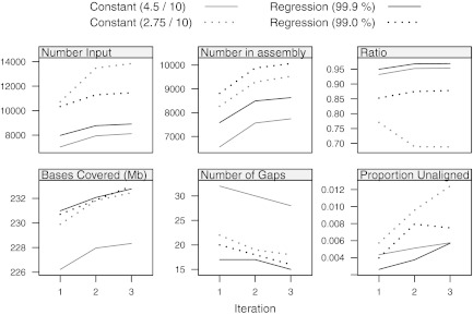
Standardized alignment scores improve assemblies: Fig. 7 summarizes the effect on iterative assembly of four filtering strategies: two regression cutoffs with different nominal specificities (99.9% and 99.0%), and two variants of the modified-constant approach previously used. (The modified-constant cutoff [s = 2.75, n = 10] allows roughly the same number of Rmaps in the first step as the 99.0% regression cutoff.) The results represent assemblies of chromosome 2 using the CHM dataset (which is independent of the dataset used to estimate parameters of the regression cutoff). To allow partial alignments at the boundary of the reference, “aligned length” and “count” are used as surrogates for length and number of fragments, which effectively make the regression cutoffs more conservative than their nominal specificities would suggest.

FIG. 7.

Comparison of significance strategies through the iterative assembly procedure. Chromosome 2 is assembled using the CHM data and the SOMA score. Two versions of the regression-based cutoff, with nominal specificities of 99.9% and 99.0%, are compared with the modified-constant schemes. (Top) The top row reports the number of Rmaps that aligned and were consequently fed into the assembly step, and the number (and proportion) of these Rmaps that were represented in the assembly. (Bottom) In the bottom row, we attempt to assess the quality of the assembly by aligning the consensus assembly to the original in silico reference. The first two panels graph the number of bases in the reference covered and the numbers of gaps; the third panel shows a crude measure of the false positive rate, namely, the proportion of bases in the consensus assembly that do not align to the reference.

A simple measure of the success of an alignment strategy is the the proportion of Rmaps passing the alignment step that are included in the ultimate assembly. The higher the better, as the set of aligned maps exhibit a high level of internal consistency when successfuly assembled. By this retention ratio, the regression cutoffs perform better than the modified-constant cutoffs with a comparable number of input Rmaps (Fig. 7, upper panel). Other quality measures that consider bases covered by the assembly, gaps, and unaligned Rmaps consistently favor alignment cutoffs by the regression approach rather than the modified-constant approach (Fig. 7, lower panel).

3.2. Alignment probability

Even if all declared alignments are correct, the set of inferred locations is a subset of the true locations because not all Rmaps successfully align. The probability that an Rmap successfully aligns depends in part on the origin of the Rmap. Understanding this dependence is necessary to normalize observed coverage; for example, increased coverage in a region could be due to increased copy number of the underlying genome, but could also be due to increased alignment probability of Rmaps from that region.

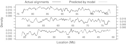
The location-specific alignment rate can be estimated using Monte Carlo simulation of noisy Rmaps from a normal reference map followed by alignment, thus replicating the pipeline actual Rmaps go through. The most time consuming step in this process is alignment. As an alternative that bypasses alignment, we considered the logistic regression model (2), where the probability of an Rmap being aligned is modeled as a function of the self-alignment score . We estimated the parameters of this model using the 50,000 simulated Rmaps mentioned previously; the predictor is the self-alignment score, with the response indicating whether the optimal score exceeded the regression cutoff with nominal specificity of 99.9%. The fitted model was then used to estimate the alignment probability for a new set of Rmaps simulated from chromosome 14, for which actual alignments were also obtained. Figure 8 compares the kernel density estimate obtained from the aligned locations with the estimated density of the true locations of all simulated Rmaps weighted by their estimated alignment probabilities. The densities estimated by the two methods are close, suggesting that we can do away with the alignment step without substantial drawbacks.

FIG. 8.

Comparison of empirical and predicted alignment rates. The probability that an Rmap will be successfully aligned depends on the origin of the Rmap. The (relative) fluctuation in the alignment rate as a function of location is an important quantity, but its estimation requires alignment of many simulated maps, which is computationally expensive. Here we assess the performance of an approximate method. The data are roughly 10,000 simulated Rmaps from human chromosome 14. The first curve is the kernel density estimate of locations obtained from alignments declared significant; this density can be used as a relative alignment rate. The second curve is the density of the true locations of the same simulated Rmaps, but with weights given by model (2). The alignment-free method provides an accurate approximation.

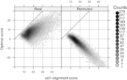
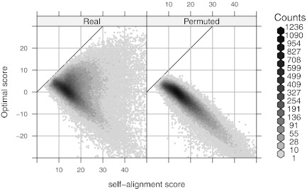
The self-alignment score can also help filter Rmaps. Figure 9 plots optimal scores for the 50,000 simulated Rmaps when aligned to the real and a permuted reference map, against their self-alignment scores. The two scatter clouds are distinctly different, overlapping only for low . The logistic regression model (2) serves to quantify this phenomenon; Rmaps in the overlapping area have low alignment probability. To save computational resources, we might consider removing Rmaps with low predicted alignment probability prior to alignment. More interestingly, the analogous plots for real Rmap data, shown in Figure 10, exhibit different behavior: for many Rmaps with high , the optimal score with the real reference seems to follow the spurious score distribution. These could be low quality Rmaps, but could also arise from regions not represented in the reference genome and thus contain novel information about the sampled genome. The set of Rmaps that have high predicted alignment probability but do not actually align are likely to be richer in such interesting Rmaps.

FIG. 9.

Optimal scores with the real and a permuted reference map are plotted against for 50,000 simulated Rmaps. The solid diagonal line represents the ideal score for an Rmap, had it been completely error free.

FIG. 10.

Analogue of Figure 9 for real Rmaps. Optimal scores with the real and a permuted reference map are plotted for each GM07535 Rmap against alignment score with itself. Possible explanations for the differences are explored in the text.

4. Discussion

Alignment is a fundamental, but not fully solved problem in optical mapping. Prior work has focused primarily on the score functions for use in dynamic programming algorithms. Here we have proposed a framework to study the distribution of spurious optimal scores, from any given score function, in order to reduce alignment errors and improve assembly of large genomes. We have also noted the utility of the self-alignment score of an Rmap in providing an a priori estimate of alignment probability, which can be used to normalize observed coverage and filter Rmaps.

The methods presented are not restricted to a specific score function. Figure 3 plots the best spurious ungapped global alignment score against two permuted references using the likelihood ratio (LR) score proposed by Valouev et al. (2006). The correlation is weaker than with the SOMA score, but an Rmap specific cutoff is still more appropriate than a constant cutoff. We apply the direct approach as before with n = 4 replications to estimate . The results, shown in Table 2, indicate that at least for the particular sets of parameters used, the SOMA score is more sensitive at a comparable specificity. This is somewhat surprising, since the LR score is based on a formal likelihood ratio test whereas the SOMA score is largely heuristic. Numerical experiments (not shown) suggest that this is due at least in part to the sizing model used by Valouev et al. (2006), which does not consider scaling errors and consequently underestimates the marginal sizing variance for large fragments.

Table 2.

Percentage of GM07535 Rmaps (Out of 206,796) Declared as Significant by the SOMA and LR Scores Using the Direct Approach

	Nominal specificity
Score function	99.0%	99.9%
SOMA	34.47	26.01
LR	26.09	18.84

Our choice of null hypothesis deserves comment. Formally, we test the hypothesis that the observed Rmap is independent of the reference map. However, it is not unlikely for an Rmap, especially a short noisy one, to originate from somewhere in the reference but have its optimal alignment somewhere else; the null hypothesis of independence is not true in such a case, yet we would not want to declare the optimal alignment significant. The hypothesis we really want to test is that the optimal alignment is a spurious alignment. Unfortunately, there are problems with this approach. Even when the optimal alignment correctly identifies the origin of a Rmap, the alignment itself may not be completely correct; so, when is an alignment sufficiently different from the true alignment to be considered spurious? Should alignments to incorrect but homologous regions be considered spurious? These issues are avoided by formulating the problem as a test of independence, as is common in alignment literature (Doolittle, 1981; Karlin and Altschul, 1990; Mitrophanov and Borodovsky, 2006). The case of a short noisy Rmap described above is not problematic in practice, as the optimal score (as well as the correct alignment score) will rarely exceed the significance threshold obtained under the null hypothesis of independence, even though that null is not strictly true.

Valouev et al. (2006) suggest a model-based approach to determine significance that is similar to ours. They postulate that the fragment lengths in the reference genome are i.i.d. exponential variates, and describe a conditional model for Rmaps given the reference. These are then used to derive the marginal distribution of Rmaps, which reduces to an i.i.d. exponential distribution for the Rmap fragment lengths, but with a different rate. Cutoffs are obtained by simulating both reference and Rmaps under the null hypothesis of independence. This is a valid approach, but it may be sensitive to parameter estimates as well as model misspecification, which is a legitimate concern since the conditional model excludes certain known sources of noise, namely desorption and scaling. Our conditional non-parametric approach bypasses these concerns. On the other hand, our permutation strategy relies on fragment lengths being i.i.d. from some distribution, not necessarily the exponential. While we expect some degree of among-fragment dependence, the empirical findings indicate that this dependence is relatively weak (Fig. 1).

Estimating the mean spurious score separately for each Rmap is usually feasible and more powerful than regression. However, for alignments involving only part of an Rmap, a cutoff based on the full map is not appropriate. This is a concern particularly for overlap matches, where alignments overhanging at the boundary of the reference map are allowed. The regression approach can still be used in such cases by considering only the aligned portion of the Rmap. The regression on N and L as used above is of course not the only possible model, but Table 1 suggests that it explains most of the Rmap-specific variation in the SOMA score. The direct non-parametric approach is an important exploratory tool (e.g., when comparing scores or deciding what parameters to use), but the regression approach is more practical for regular use.

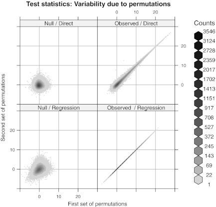
Our use of a limited number of permutations is essential but somewhat unusual, in the sense that the test statistics include Monte Carlo variation. This raises the question: how many permutations are sufficient and how do they affect the inference? In our examples, six permutations of the reference define the test: four to estimate one to estimate model parameters, and another to obtain empirical cutoffs. Figure 11 shows the effect of using two separate sets of these six permutations. In the direct approach, even with this small number of permutations, the variability in the observed statistics is mild compared to the variability inherent in the null distribution. This variability can be further reduced by using more permutations to estimate the mean spurious scores. It is even less of a concern in the regression method, which is the approach used in practical tasks.

FIG. 11.

Variability in test statistics due to permutations. Two separate sets of permutations are used to derive the test statistics and . (Left) The left panel represents realizations of T₁ and T₂ from the null distribution. (Right) The right panel shows their observed values. Ideally, the observed values should not depend on the permutations used. Not surprisingly, this holds for the regression approach but not the direct approach. However, even with only four permutations to estimate , the variability in the latter is mild compared to the variability inherent in the null distribution. The panels corresponding to the null distributions indicate that unlike T₁, T₂ retains some Rmap-specific component.

In this article, we have addressed the question of significance of Rmap alignments to a reference map. Significance of alignments are determined by their scores. Our primary goal was to obtain the null distribution, with as few assumptions as possible, of the optimal alignment score of an Rmap given any score function. We achieved this using alignments to permutations of the reference map, and developed conditional permutation tests for significance with control over error rates. This approach was further simplified to obtain simple Rmap specific score cutoffs that have been validated using simulation and through use in iterative assembly. We have outlined ways to use this approach to compare different score functions. Our investigations have also provided new insight into the nature of optical map data and led to a Rmap-specific summary score that may help simplify certain aspects of optical map analysis.

5. Appendix

5.1. Score functions for alignment

Let and denote two restriction Rmaps with m and n fragments respectively. Let the corresponding representations in terms of cut sites be and . An alignment between x and y can be represented by an ordered set of index pairs

indicating a correspondence between the cut sites and for , where and . To align the two Rmaps, one defines an objective function that assigns a score to all possible alignments and then tries to find the alignments that give the optimal or nearly optimal scores. For a certain class of score functions that satisfy the additive property

this search can be performed efficiently using variants of the Needleman-Wunsch and Smith-Waterman dynamic programming algorithms. Non-additive score functions may be appropriate in certain situations, but have not been investigated.

The sensitivity with which alignments can detect locations of Rmaps depends primarily on the score function used. Different scores are appropriate for different types of alignments. A natural approach to derive score functions is to base it on model-based likelihood ratio tests (Altschul, 1991). Such scores have most recently been derived by Valouev et al. (2006) for alignment of two Rmaps (both being subject to noise), as well as for Rmaps against an noise-free reference map. The model they use is in essence similar to the one described in Sarkar (2006), but excludes desorption and scale errors. We refer the reader to the original article for details.

Another score function for Rmap to reference map alignment has been developed as part of the SOMA software suite (Kohn, 2003). Although this score is largely heuristic, it has been used quite extensively and successfully. Since there is no published reference, we give some details here. The score of the full alignment is determined by the score of each chunk . Let ν be the length of the reference map in the chunk, and x be the corresponding Rmap length. Further, let m = i_ℓ − i_ℓ-1 be the number of reference map fragments combined to form length ν, and n = j_ℓ − j_ℓ-1 be the number of Rmap fragments combined to form length x (thus, u = m − 1 is the number of missing cut sites and v = n − 1 the number of false cut sites). Then, the contribution of this chunk to the final score is given by

(3)

where P_m is a missing cut penalty, P_f is a false cut penalty, C(ν) is a sizing error cutoff (related to the variance of the sizing errors) and λ represents the mean reference fragment length. The log term is intended to give higher weight to longer fragments. A critical component of the score is the choice of C(ν); empirically, a form piecewise linear in ν² has been found to be useful. This is consistent with the marginal sizing variance derived in Sarkar (2006) and can be viewed as an approximation to the latter, more recent, form. A further adjustment intended to correct for desorption is used as follows: instead of counting each missing cut site as one to give a total of u = m − 1, each missing cut contributes the quantity π(y), the probability of retaining a fragment of size y, where y is the distance from the missing cut site to the nearest observed cut site. Unlike the likelihood ratio based scores, there is no natural interpretation for the score of the complete alignment, which is simply the sum of the scores for individual aligned chunks.

5.2. Iterative assembly

Gentig produces highly accurate assemblies of bacterial genomes. However, it does not scale to genomes of mammalian size because the algorithm is quadratic and there is no obvious way to parallelize it. One solution is a heuristic assembler which uses pairwise Smith-Waterman alignment (Kohn, 2003; Valouev et al., 2006) to subdivide the assembly problem in many smaller problems and uses Gentig as the low-level assembly engine (Mullikin and Ning, 2003). The computational work for both the alignment and assembly steps is distributed over a large network of clustered workstations (Litzkow et al., 1988).

The algorithm is iterative, and the output of each step of the iteration is an approximate map of the genome. In the subsequent step, this approximation is used as the reference map against which all the Rmaps in the dataset are aligned. Then the Rmaps are clustered according to the location of their alignments to the reference, and each cluster is assembled locally. The consensus maps from these assemblies give rise to the reference map for the next step.

The algorithm emerged from the following reasoning. Within species, we expect a high degree of genomic conservation punctuated by structural variants that are commonly spanned by long Rmaps. Consequently, in a region of the genome where the differences between the target genome and the reference are minor, Rmaps tend to align (because the dynamic programming scoring function is designed to tolerate optical mapping errors and minor differences are typically in the domain of that error model). The data, then, can drive the approximation in the right direction within that region by assembling the Rmaps that align there. In a non-conserved region of the genome, Rmaps tend not to align to the in silico map, and so a gap can be opened in the first iteration. The subsequent steps allow the gap to be bridged by walking into it from the conserved flanks.

The quality of an assembly is a function of the extent of the coverage of the genome by the consensus maps and of the accuracy of the consensus maps. That accuracy, in turn, is a function of the depth of the Rmap coverage within the contigs. To achieve a high quality assembly, we stringently control the input to and output from the local assembly phase at each step in the iteration. The goal of these controls is to correctly place Rmaps within the contigs, even at the expense of diminishing the depth or extent of coverage because an incorrectly placed Rmap could introduce errors in the consensus. In subsequent steps of the iteration, these errors could be reinforced and propagated.

We implemented the controls as follows for the experiment described in Section 3.1:

• • Input to local assembly

  • ○ Pairwise alignment threshold: We used two regression cutoffs with nominal specificities 99.9% and 99.0%. An alignment was accepted if the score exceeded (9.711 − 0.216N − 0.014L −0.0001546NL) + κ(12.010742 − (9.711 − 0.216N − 0.014L − 0.0001546NL)), where κ = 0.401 in the first case, and 0.273 in the second case. These cutoffs are derived using the regression method as discussed in the text.

• • Output from local assembly

  • ○ Minimum number of Rmaps in a contig: Contigs must be supported by at least five Rmaps in order to be propagated to the next iteration.

  • ○ Consensus map trimming: The ends of consensus maps were trimmed so that the first and last fragments were supported by at least four Rmaps.

5.3. Simulation model

Rmaps were simulated from the in silico reference genome using the parametric generative model described below. Sarkar (2006) discusses the model and parameter estimation in greater detail.

Origins were selected uniformly from the reference genome. The total length of the Rmaps followed a left-truncated exponential distribution with a minimum size of 300 kb and average size of 440 kb. Small fragments are rarer in Rmaps than in the reference. To model this, fragments less than 400 bp were merged with neighboring fragments, and remaining fragments were dropped with probability 1 − e^-αμ, where μ is the size of the fragment, and α was chosen so that a fragment of size 1.35 kb was dropped with probability 0.5. The reported size of a fragment of length μ was computed as X = RZ, where

reflects the image processing error in measuring length and

is a Rmap-specific “rubber-banding” factor that reflects local uncertainty in the estimated scale factor. Whether true cut sites are identified (success) or not (failure) is modeled as independent Bernoulli trials, with probability p = 0.75 of success. False cuts, that is, apparent restriction sites that correspond to no restriction site in the true Rmap, are modeled as a homogeneous Poisson process, with rate ζ = 0.002 per kb of DNA.

Acknowledgments

We thank Christina Kendziorski, Michael Waterman, and Anton Valouev for helpful discussions. This work was supported in part by funding from the National Institutes of Health grants R01-CA64364 to M.A.N. and R01-HG00225 to D.C.S.

Disclosure Statement

No competing financial interests exist.

References

- Altschul S.F. Amino acid substitution matrices from an information theoretic perspective. J. Mol. Biol. 1991;219:555–565. doi: 10.1016/0022-2836(91)90193-A. [DOI] [PMC free article] [PubMed] [Google Scholar]
- Anantharaman T.S. Mishra B. Schwartz D.C. Genomics via optical mapping. III: contiging genomic DNA. Proc. Int. Conf. Intell. Syst. Mol. Biol. 1999:18–27. [PubMed] [Google Scholar]
- Antonacci F. Kidd J.M. Marques-Bonet T., et al. A large and complex structural polymorphism at 16p12.1 underlies microdeletion disease risk. Nat. Genet. 2010;42:745–750. doi: 10.1038/ng.643. [DOI] [PMC free article] [PubMed] [Google Scholar]
- Carr D. B. Littlefield R. J. Nicholson W. L., et al. Scatterplot matrix techniques for large N. J. Am. Stat. Assoc. 1987;82:424–436. [Google Scholar]
- Cox D. R. Hinkley D. V. Theoretical Statistics. Chapman & Hall Ltd; London: 1979. [Google Scholar]
- Dimalanta E. Lim A. Runnheim R., et al. A microfluidic system for large DNA molecule arrays. Anal. Chem. 2004;76:5293–5301. doi: 10.1021/ac0496401. [DOI] [PubMed] [Google Scholar]
- Doolittle R. F. Similar amino acid sequences: chance or common ancestry? Science. 1981;214:149–159. doi: 10.1126/science.7280687. [DOI] [PubMed] [Google Scholar]
- Huang X. Waterman M. S. Dynamic programming algorithms for restriction map comparison. Comput. Appl. Biosci. 1992;8:511–520. doi: 10.1093/bioinformatics/8.5.511. [DOI] [PubMed] [Google Scholar]
- Karlin S. Altschul S. F. Methods for assessing the statistical significance of molecular sequence features by using general scoring schemes. Proc Natl. Acad Sci. USA. 1990;87:2264–2268. doi: 10.1073/pnas.87.6.2264. [DOI] [PMC free article] [PubMed] [Google Scholar]
- Kidd J. Cooper G. Donahue W., et al. Mapping and sequencing of structural variation from eight human xsgenomes. Nature. 2008;453:56–64. doi: 10.1038/nature06862. [DOI] [PMC free article] [PubMed] [Google Scholar]
- Kohn S. SOMA: Software for Optical Map Analyis. 2003. Personal communication.
- Lim S. A. University of Wisconsin; Madison: 2004. Single molecule systems: advancements and applications to microbial and human genome analysis [Ph.D. dissertation] [Google Scholar]
- Litzkow M. Livny M. Mutka M. Condor—a hunter of idle workstations. Proc. 8th Int. Conf. Distributed Comput. Syst. 1988:104–111. [Google Scholar]
- Mitrophanov A. Y. Borodovsky M. Statistical significance in biological sequence analysis. Brief Bioinform. 2006;7:2–24. doi: 10.1093/bib/bbk001. [DOI] [PubMed] [Google Scholar]
- Mullikin J. C. Ning Z. The phusion assembler. Genome Res. 2003;13:81–90. doi: 10.1101/gr.731003. [DOI] [PMC free article] [PubMed] [Google Scholar]
- Sarkar D. University of Wisconsin; Madison: 2006. On the analysis of optical mapping data [Ph.D. dissertation] [Google Scholar]
- Scherer S. W. Lee C. Birney E., et al. Challenges and standards in integrating surveys of structural variation. Nat. Genet. 2007;39:S7–S15. doi: 10.1038/ng2093. [DOI] [PMC free article] [PubMed] [Google Scholar]
- Schnable P. Ware D. Fulton R., et al. The b73 maize genome: complexity, diversity, and dynamics. Science. 2009;326:1112–1115. doi: 10.1126/science.1178534. [DOI] [PubMed] [Google Scholar]
- Schwartz D. C. Li X. Hernandez L., et al. Ordered restriction maps of Saccharomyces cerevisiae chromosomes constructed by optical mapping. Science. 1993;262:110–114. doi: 10.1126/science.8211116. [DOI] [PubMed] [Google Scholar]
- Sebat J. Lakshmi B. Troge J., et al. Large-scale copy number polymorphism in the human genome. Science. 2004;305:525–528. doi: 10.1126/science.1098918. [DOI] [PubMed] [Google Scholar]
- Teague B. Waterman M. S. Goldstein S., et al. High-resolution human genome structure by single-molecule analysis. Proc Natl. Acad. Sci. USA. 2010;107:10848–10853. doi: 10.1073/pnas.0914638107. [DOI] [PMC free article] [PubMed] [Google Scholar]
- Valouev A. Li L. Liu Y., et al. Alignment of optical maps. J. Comput. Biol. 2006;13:442–462. doi: 10.1089/cmb.2006.13.442. [DOI] [PubMed] [Google Scholar]
- Zhou S. Bechner M. C. Place M., et al. Validation of rice genome sequence by optical mapping. BMC Genomics. 2007;8:278. doi: 10.1186/1471-2164-8-278. [DOI] [PMC free article] [PubMed] [Google Scholar]
- Zhou S. Wei F. Nguyen J., et al. A single molecule scaffold for the maize genome. PLoS Genet. 2009;5:e1000711. doi: 10.1371/journal.pgen.1000711. [DOI] [PMC free article] [PubMed] [Google Scholar]