Modeling Plan-Related Clinical Complications using Machine Learning Tools in a Multi-Plan IMRT Framework

Abstract

Purpose

To predict organ-at-risk (OAR) complications as a function of dose-volume (DV) constraint settings without explicit plan computation in a multi-plan IMRT framework.

Methods and Materials

A large number of plans were generated by varying the dose-volume constraints (input features) on the OARs (multi-plan framework), and the dose-volume levels achieved by the OARs in the plans (plan properties) were modeled as a function of the imposed dose-volume constraint settings. OAR complications were then predicted for each of the plans by using the imposed dose-volume constraints alone (features) or in combination with modeled dose-volume levels (plan properties) as input to machine learning (ML) algorithms. These ML approaches were used to model two OAR complications following head-and-neck and prostate IMRT, xerostomia and Grade 2 rectal bleeding. Two-fold cross-validation was used for model verification and mean errors are reported.

Results

Errors for modeling the achieved dose-volume values as a function of constraint settings were 0-6%. In the head and neck case, the mean absolute prediction error of the saliva flow rate normalized to the pre-treatment saliva flow rate was 0.42% with a 95% confidence interval of [0.41%, 0.43%]. In the prostate case, an average prediction accuracy of 97.04% with a 95% confidence interval of [96.67%, 97.41%] was achieved for Grade 2 rectal bleeding complications.

Conclusion

ML can be used for predicting OAR complications during treatment planning allowing for alternative dose-volume constraint settings to be assessed within the planning framework.

I. INTRODUCTION

Radiation treatment planning requires consideration of competing objectives: maximizing the radiation delivered to the planning target volume (PTV) and minimizing the amount of radiation delivered to all other tissues. The tradeoff between the above factors leads to consideration of multi-criteria objective techniques [1-7]. Recent papers addressing this topic include Gopal and Starkschall [1], which presents various two-dimensional plan comparison visualizations, Rosen et al., which deals with conformal radiotherapy and emphasizes graphically-guided adjustments to base plans [2], Zhang et al., which focuses on sensitivity analysis issues [3] and, as in the earlier work by Yu [4] and by Xing et al [5] develops mechanisms for multi-parametric adjustments that seek to construct a sequence of treatment plans that converge to a pre-specified set of goals, Romeijn et al. which shows the mathematical equivalence of Pareto surfaces based on alternative metrics [6], and Craft et al., which discusses invariance properties of Pareto surfaces [7]. The Pareto surface is applied to IMRT cases via a two-step procedure, in which one plan is generated through optimization and subsequent plans are generated based on the single plan and satisfaction of the constraints [8, 9]. Despite the above literature, the limitation of the current planning approach is that the relationship between the achieved plan dose-volume (DV) or dose levels and the DV or dose constraint settings is not known apriori. Further, the current planning approach does not allow for inferential determination of the ideal DV constraint settings that will yield desired outcomes (achieved DV levels or plan-related complication levels).

We have previously described a multi-plan framework which provides for the generation of many plans that differ in their DV constraint settings [10]. We utilize this framework in this work. The rationale for this work is: (1) DV constraints are implicitly handled by optimization algorithms in commercial planning systems as inequalities through the introduction of penalty variables. These penalty variables account for differences between the actual plan DV values and the DV constraint settings. As a result, the achieved DV levels for an organ-at-risk (OAR) are frequently not equal to the DV constraint settings even in the case that the constraint settings for that OAR are met. (2) Altering the DV constraint settings for a given OAR has an effect on the actual DV values corresponding to all involved OARs in the clinical case even if the DV constraint settings on the other OARs are unchanged. (We have previously shown in Meyer et al [10] that the achieved DV level for a given OAR can be accurately modeled as a quadratic function of the DV constraint settings corresponding to all involved OARs.) (3) Without a suitable knowledge base of plans for a given patient it is generally impossible to determine the DV constraint setting ranges for each OAR that will yield the desired output DV values (and consequently OAR complications). It would be ideal if the computation of a limited number of plans combined with suitable modeling tools enabled the construction of a plan surface representing DV levels for a given OAR as a function of DV constraint settings corresponding to all involved OARs. Taking into consideration (1)-(3) we seek to predict OAR complications on the basis of the DV constraint settings (without explicit plan computation for those settings), thereby guiding the selection of OAR constraint settings for all involved OARs.

The purpose of this work is to describe an approach to guide the selection of DV constraint settings by predicting plan-related OAR complications (and achieved DV levels as an intermediate step) as a function of DV constraint settings directly without explicit plan computation. We hypothesize that such a prediction is possible using machine learning (ML) algorithms. We selected two frequently encountered OAR complications: xerostomia in head and neck IMRT and rectal bleeding in prostate IMRT.

II. METHODS AND MATERIALS

A. Multi-Plan Framework

We first describe the generation of the multi-plan framework that serves as a knowledge base to be used in both training (i.e., model development) and validation (i.e., establishment of confidence intervals) of the prediction of one OAR complication as a function of DV constraints corresponding to all involved OARs. A large number of plans were explicitly generated (for each case) by varying the input dose and DV constraint settings for two test clinical cases: head and neck IMRT and prostate. Figures 1 (a) and (b) show the transverse sections of two test clinical cases.

Figure 1.

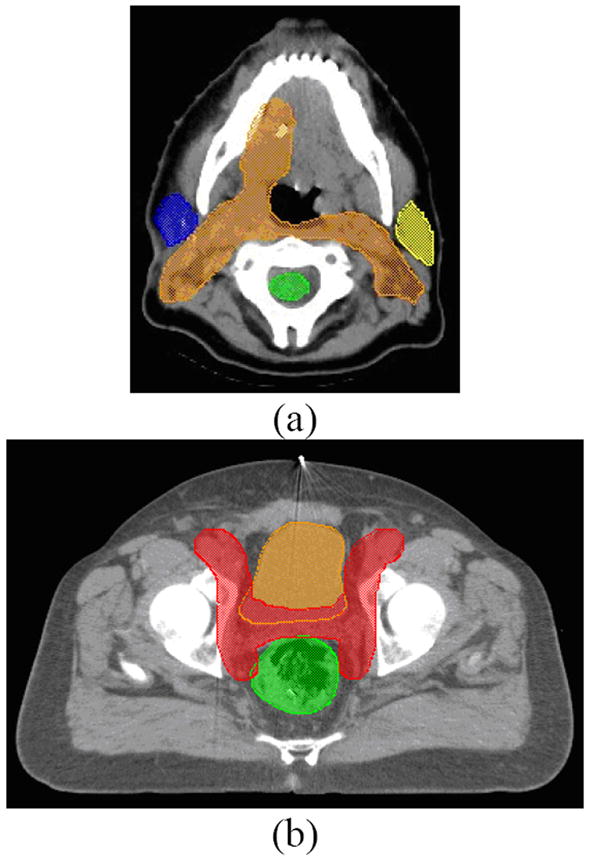
Axial slices of the (a) head-and-neck case showing the planning target volume (PTV), parotids, and spinal cord, and (b) prostate case showing the PTV, bladder, and rectum.

A.1 Head and Neck Case

For one head and neck case, 125 plans were generated by varying the DV constraints on the left parotid (LP), right parotid (RP) and cord. For each OAR, 5 sets of DV constraints were considered (see Table 1). Plans were normalized so that 90% of the PTV received 50.4 Gy. Figure 2 show the 125 DVHs corresponding to 125 plans.

Table 1.

Variation of DV constraint settings for head and neck and prostate cases.

	DVH Constraint Settings
Head and Neck	66% Left Parotid	33% Left Parotid	66% Right Parotid	33% Right Parotid	Max Cord
	20-32 Gy in 3 Gy increments	26-38 Gy in 3 Gy increments	20-32 Gy in 3 Gy increments	26-38 Gy in 3 Gy increments	33-45 Gy in 3 Gy increments
Whole Pelvis	25% Bladder	50% Bladder	25% Rectum	50% Rectum	30% Bowel
	41-47 Gy in 3 Gy increments	35-41 Gy in 3 Gy increments	38-44 Gy in 3 Gy increments	31-37 Gy in 3 Gy increments	11-17 Gy in 3 Gy increments
Prostate	25% Bladder	50% Bladder	25% Rectum	50% Rectum
	29-30 Gy	25-26 Gy	27-28 Gy	24-25 Gy

Figure 2.

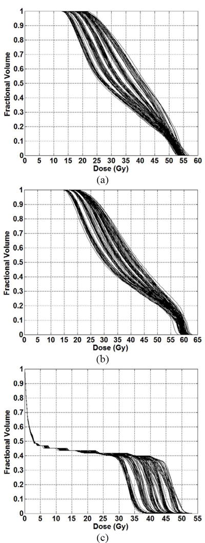
DVHs corresponding to full knowledge base (encompassing both training and testing datasets) of 125 head and neck plans for the (a) left parotid and (b) right parotid and (c) spinal cord.

A.2 Prostate Case

For one prostate case, 256 plans were generated by varying the DV constraints on the rectum, bladder and bowel. An initial set of 64 plans were generated in which the target involved the prostate plus nodal volumes (prescription dose of 45 Gy). Four prostate-only boost plans were generated (prescription dose of 30.6 Gy). The combination of initial and boost plans resulted in 256 plans (plans were normalized so that 95% of the PTV associated with the prostate received 75.6 Gy). The DV constraints are summarized in Table 1. Figure 3 shows the DVHs corresponding to 256 plans.

Figure 3.

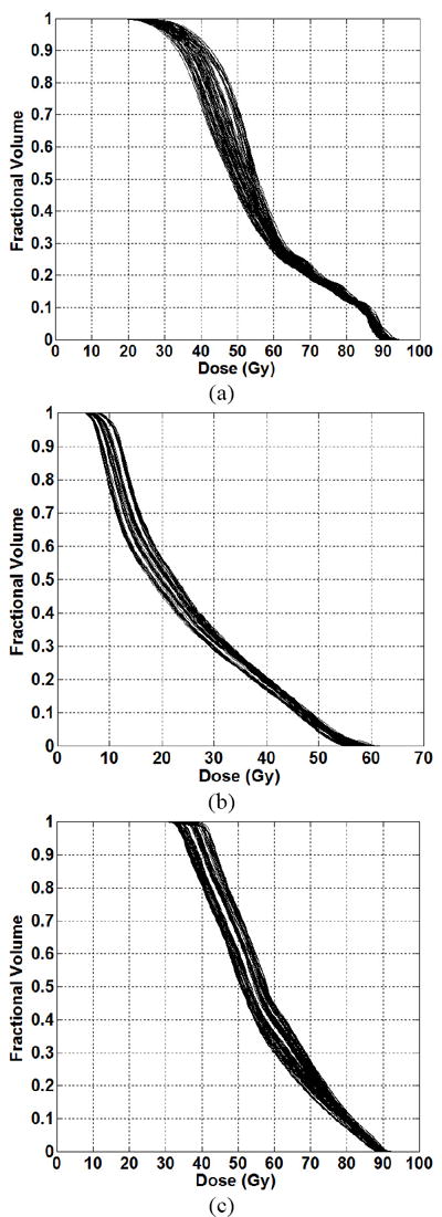
DVHs corresponding to full knowledge base (encompassing both training and testing datasets) of 256 prostate plans for the (a) bladder and (b) bowel and (c) rectum.

B. Dose-Volume Relationships to OAR complications

Previous reports have described the relationships (derived retrospectively) between plan DV levels and OAR complications. These data served as the “ground truth” for the actual calculation of OAR complications against which our prediction of OAR complications was compared.

B.1 Saliva Flow Rate

Retrospective studies have shown that specific volumes of the parotid glands (66%, 45% and 24%) receiving specific doses (15 Gy, 30 Gy and 45 Gy) correlated with post-treatment saliva flow rate [11-13]. Chao et al presented an EUD-based model to calculate post-treatment saliva flow rate [12], which we use as the ground truth for each of the 125 plans.

The saliva flow rate (mL/min) is normalized to that before treatment. The model is

$$F=[\exp (-A·{\mathit{EUD}}_R-B·{\mathit{EUD}}_R^2)+\exp (-A·{\mathit{EUD}}_L-B·{\mathit{EUD}}_L^2)]/2$$ (1)

where A and B are fitted parameters (0.0315 and 0.000168 respectively), F is the expected resulting fractional saliva output, and EUD is the equivalent uniform dose to the left (L) and right (R) parotids as defined in equation (2).

$$\mathit{EUD}={\left(\frac{1}{N}\sum _{i=1}^N{D}_i^a\right)}^{1/a}$$ (2)

where, N is the total number of voxels corresponding to a given structure, D_i is the dose to the ith voxel, and a =1, is a structure-specific parameter that describes the dose–volume effect.

B.2 Rectal Bleeding

Retrospective studies have shown a correlation between rectal bleeding and 25-70% of the rectal volume receiving 60-75 Gy [14-19] (25-30% for 70 Gy, the most often cited DV level). Therefore, we used a threshold of 25%/70 Gy to determine a binary classification for the plans in the prostate case. The volume of 25% also corresponds to one of the rectum DV constraint settings in this work.

C. Modeling the Plan Surface

Our goal is to predict OAR complications (referred to as labels) during the treatment planning process as a function of the DV constraint settings (referred to as features) corresponding to all involved OARs. In some cases, in order to accurately predict treatment related complications, an intermediate step of modeling achieved plan DV levels (referred to as plan properties) corresponding to one OAR as a function of DV constraint settings (features) for the full set of OARs is employed (equation 3):

$$\mathit{plan}{\mathit{properties}}_{\mathit{OARi}}=f({\mathit{features}}_{\mathit{OAR}\mathit{1}},{\mathit{features}}_{\mathit{OAR}\mathit{2}},\dots \dots ,{\mathit{features}}_{\mathit{OARn}})$$ (3)

where i corresponds to the OAR whose plan properties are being modeled and n corresponds to the number of involved OARs. Details of modeling plan properties as a function of features were described previously in Meyer et al [10]. This intermediate modeling step was utilized in the head and neck case. Plan properties (specifically dose to 24%, 45% and 66% of the parotids were modeled as a function of the input constraint settings (features) in Table 1 using quadratic functions and via linear programming data fitting tools as described in [10].

D. Machine Learning (ML) Algorithms

We use ML algorithms to predict treatment related complications for an OAR as a function of DV constraint settings (features) corresponding to all involved OARs and modeled achieved plan dose and dose-volume levels (plan properties) corresponding to the OAR in question if necessary as input (equation 4).

$${\mathit{complications}}_{\mathit{OARi}}=g({\mathit{features}}_{\mathit{OAR}\mathit{1}},{\mathit{features}}_{\mathit{OAR}\mathit{2}},\dots \dots ,{\mathit{features}}_{\mathit{OARn}},\mathit{plan}{\mathit{properties}}_{\mathit{OARi}})=g(\mathit{features},f(\mathit{features}))$$ (4)

The goal of ML in this work is to build and validate the numerical prediction or decision models (described in equation 4) from the knowledge base. The knowledge base is the collection of plans arising from our multi-plan framework coupled with properties of those plans.

The details of the modeling process are summarized in Figure 4. The outputs of the ML models (labels) are the plan-related OAR complications. In our work, features alone served as the input parameters in the ML model used to predict labels (as in the prostate case) if acceptable prediction accuracy was achieved (solid path). Otherwise, these inputs were supplemented by modeled plan properties (achieved DV levels), i.e., dashed path. In summary, 11 inputs (5 features, and 3 predicted plan properties for each parotid) were used to predict saliva flow rate in the head and neck case and 5 inputs (5 features) were used to predict Grade 2 rectal bleeding complication in the prostate case using ML. These inputs to the ML algorithms are summarized in Table 2.

Figure 4.

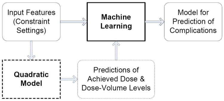
Summary of Modeling Process Summary involving ML prediction of OAR complications using features and plan properties (if necessary).

Table 2.

Input variables used in modeling the achieved dose volume and dose levels in the head and neck case and the OAR complications in the head and neck and prostate case.

	Input Variables
Head and Neck	33% Left Parotid	66% Left Parotid	33% Right Parotid	66% Right Parotid	Max Cord
Pelvis/Prostate	25% Bladder	50% Bladder	25% Rectum	50% Rectum	30% Bowel

Both the construction and the validation of the models were accomplished through the repeated use of a two-fold cross-validation process. In this process, the knowledge base (set of all computed IMRT plans for a case) is first randomly partitioned into training and testing subsets each, consisting of an equal number of samples (plans). A model is constructed using only the subset of the data in the training subset (50% of the total number of plans), and the quality of the model is evaluated by applying it to the data in the testing subset (data not included in the training subset) and assessing the accuracy of the results produced on that subset. This process was repeated 50 times and the average errors along with 95% confidence intervals are reported.

Two machine learning algorithms were explored: support vector machines (SVM) and decisions trees. While both approaches were tested for each of the two cases, it was determined that SVMs yielded superior results in predicting saliva flow-rate and decision trees yielded superior results in predicting rectal bleeding.

D.1 Sequential Minimal Optimization

The method that we used to predict the saliva flow rate from features and the modeled plan properties was the construction of a linear model (equation 4) via a sequential minimal optimization (SMO) algorithm [20, 21] for “training” a support vector regression model, which is essentially a quadratic data fitting error minimization problem whose objective function is comprised of a weighted combination of two terms: the first term is a quadratic error measure and the second is a model complexity term defined by a norm of the weights selected for the input features. The SMO algorithm employs a linear model of the form k + l u where u denotes the vector of input variables and k and l denote the fitting parameters (k a scalar, l a vector) to be generated by SMO. Training a support vector machine (SVM) is accomplished by the solution of a large constrained quadratic programming (QP) optimization problem in order to determine the optimal weights of those linear terms. In support vector regression, an accuracy threshold ε is set so that model prediction errors that are below this threshold yield a penalty of 0 in the objective function. In order to model these error thresholds functions, appropriate inequality constraints are used in the weight optimization problem:

$$\begin{array}{l}\mathrm{minimize}1/2\mathit{ll}+\mathrm{c}(\mathit{dd}+\mathit{ee})\\ \mathrm{subject\; to}-d^i-\epsilon <p^i­k-l{u}^i<\epsilon +e^i\mathrm{for}\mathrm{i}=1,\dots ,\mathrm{K},d>0,e>0\end{array}$$ (5)

where, c is a weighting factor for the sum of errors terms dd+ee and ll is a model complexity measure.

D.2 Decision Trees

The binary classification method in predicting Grade 2 rectal bleeding is an optimized decision tree, whose generation process via supervised learning we will outline below (i-v). Referencing Figure 5, note that the non-leaf nodes (that is, the nodes that have successor nodes below them, shown as ellipses in Figure 5) represent univariate inequality tests that are followed by further tests at lower nodes until the final tests leading to the leaf nodes (shown as rectangles in Figure 5) yield classification decisions [22, 23].

Figure 5.

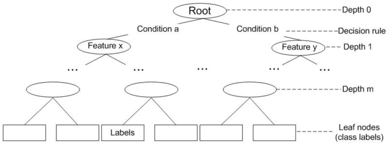
Optimized Decision Tree Algorithm Schematic.

A general approach to the construction of decision trees starts with the selection of a branching test at the root node at the top of the tree and can be summarized as following:

1. Choose an attribute-value pair that leads to the best partition of the training instances with respect to the output attribute.

2. Create a separate branch for each range of value of the chosen attribute.

3. Divide the instances into subgroups corresponding to the attribute value range of the chosen node.

4. For each subgroup, terminate the attribute partitioning process if:

   1. All members of a subgroup have the same value for the output attribute.
   2. No further distinguishing attributes can be determined. Label the branch with the output value seen by the majority of remaining instances.

5. Else, for each subgroup created in (iii) for which the attribute partitioning process is not terminated in (iv) at a leaf, repeat the above branching process.

This stage of the algorithm is based on the training data, and generally produces a large and complex decision tree that correctly classifies all of the training instances. In the second stage of the tree generation process, this decision tree is then pruned by considering the test data and removing parts of the tree that have a relatively high error rate or provide little gain in statistical accuracy.

III. RESULTS

A. Modeling Plan Properties

We used equation 4 to determine the achieved plan properties as a function of features in the head and neck case. Figures 6 and 7 show the results of modeling plan properties for the left and right parotids, respectively, i.e., the comparison between the predicted plan properties and the actual plan properties. The plan indices are reordered in each subfigure, so that the displayed delivered doses are in increasing order. This reordering is done to show the distribution of the delivered doses and to better allow comparisons of delivered doses with the corresponding doses as predicted by equation 4. Relative fit errors varied from 0 to 6%.

Figure 6.

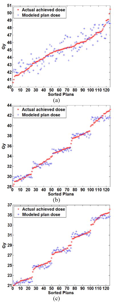
Comparison of the modeled plan dose as a function of the input constraint settings using quadratic modeling and the actual achieved dose for the left parotid at volume levels of (a) 24% (b) 45% and (c) 66%.

Figure 7.

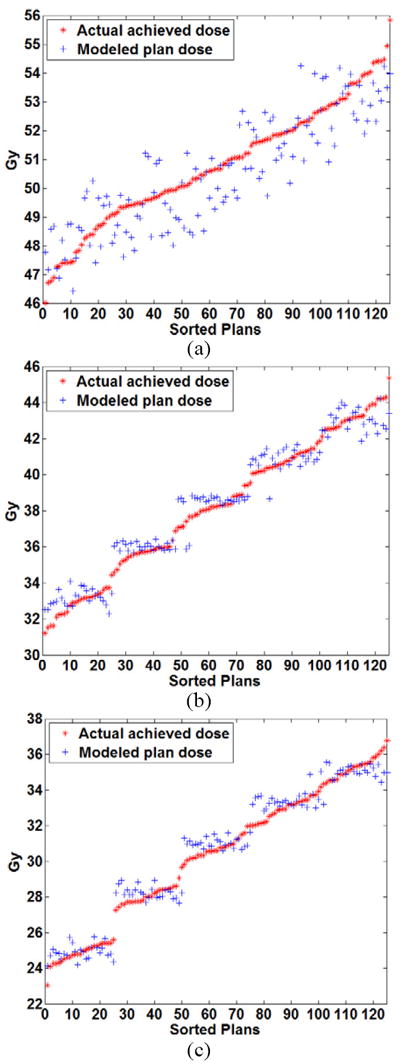
Comparison of the modeled plan dose as a function of the input constraint settings using quadratic modeling and the actual achieved dose for the right parotid at volume levels of (a) 24% (b) 45% and (c) 66%.

B. Saliva Flow Rate

The results for predicted saliva flow rate (equation 5) using the SMO algorithm are shown in Figure 8. The x-axis was the actual flow rate (normalized to the pre-treatment saliva flow rate) for each of the 125 plans in the knowledge base (plans were sorted according to increasing saliva flow-rate). The actual saliva flow rate was obtained using equation 1. The y-axis was the mean saliva flow-rate using equation 5 and obtained from the 2-fold cross-validation process. From Figure 8, it can be seen the normalized saliva flow rate ranged from 20-30% for the case considered. The further a point is from the diagonal (which represents equality of actual and predicted values), the larger the prediction error is. The mean absolute error (averaged over 50 simulations in cross-validation) for saliva flow-rate prediction obtained from the 2-fold cross-validation and normalized to the pre-treatment saliva flow rate compared with the ground truth obtained from the EUD-exponential model in equation 1 was 0.42% with a 95% confidence interval [0.41%, 0.43%].

Figure 8.

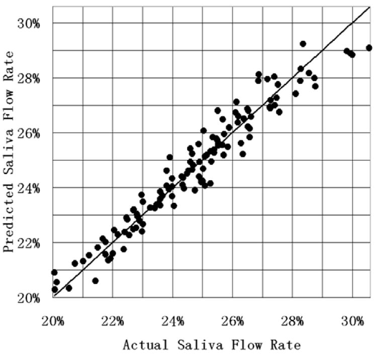
Comparison of the mean (obtained from the 2-fold cross-validation process) predicted saliva flow rate (normalized to the pre-treatment saliva flow rate) using equation 5 to the actual saliva flow rate (calculated using equation 1).

C. Rectal Bleeding

Figure 9 shows a representative decision tree resulting from 2-fold cross-validation method applied to the 256 prostate treatment plans. Each decision node of the tree represents one DVH constraint, which is an input to the planning system. For example, 25Bldr is the DVH constraint set for 25% of the bladder volume. The numbers on the branches show the dose level. Each leaf node represents a classification result, and the number in parenthesis is the number of instances that were classified correctly/incorrectly. Each leaf node corresponds to the set of inequalities on the path from the top-most node to that leaf. An example of the prediction results for a subset of 20 plans (from the set of 256 total plans) are illustrated in Table 3. The DV constraints for 20 representative plans along with the prediction of Grade 2 complication (C) or no Grade 2 complication (NC) are listed in the first six columns. The last column indicates whether the prediction was correct (Y) or incorrect (N). Using 2-fold cross validation 50 times, we achieved an average prediction accuracy of 97.04% with a 95% confidence interval of [96.67%, 97.41%] for Grade 2 rectal bleeding.

Figure 9.

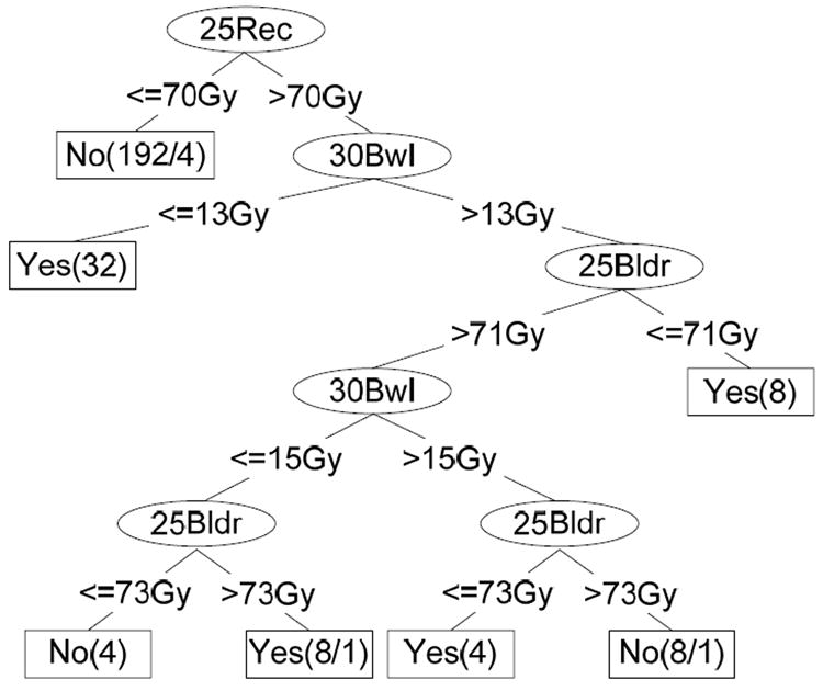
Decision Tree for Grade 2 Rectal Complication Classification – an example.

Table 3.

Illustration of prediction of Grade 2 rectal bleeding via 20 representative plans using the optimized decision tree algorithm.

	25%Bladder	50%Bladder	25%Rectum	50%Rectum	30%Bowel	C/NC	Y/N
Plan 1	70	60	66	56	11	N	Y
Plan 2	70	60	70	60	17	N	Y
Plan 3	70	60	66	56	15	N	Y
Plan 4	71	61	66	56	15	N	Y
Plan 5	72	62	70	60	13	N	Y
Plan 6	73	63	67	57	15	N	Y
Plan 7	74	64	69	59	17	N	Y
Plan 8	75	65	66	56	11	N	Y
Plan 9	76	66	65	55	17	N	N
Plan 10	76	66	68	58	17	N	Y
Plan 11	76	66	72	62	13	C	Y
Plan 12	76	66	71	61	11	C	Y
Plan 13	70	60	71	61	17	C	Y
Plan 14	71	61	72	62	15	C	Y
Plan 15	72	62	71	61	13	C	Y
Plan 16	74	64	71	61	11	C	Y
Plan 17	72	62	70	60	11	C	N
Plan 18	75	65	72	62	11	C	Y
Plan 19	76	66	72	62	15	C	Y
Plan 20	77	67	71	61	15	C	Y

D. OAR Complications As a Function of DV Constraints

Our case-specific models were used to then predict OAR complications as a function of DV constraints for arbitrary input DV constraints without explicit plan computation. Figure 10 shows an example of the results for the prediction of normalized saliva flow rate as a function of the DV constraints using the approach described in this work. The contours in each plot correspond to the percentage saliva flow rate normalized to the pre-treatment saliva flow rate as a function of DV constraint settings for two of the OARs and a fixed constraint setting for the third OAR. It can be observed that the plot for saliva flow rate as a function of the DV constraint settings on one parotid gland (left or right) and the maximum dose constraint to the cord for a fixed DV constraint setting for the other parotid gland is near linear (see Figures 10 (a) and (b)) while the plot for the saliva flow rate as a function of the DV constraints on both parotid glands for a fixed maximum cord dose constraint shows curvature (see Figure 10 (c)).

Figure 10.

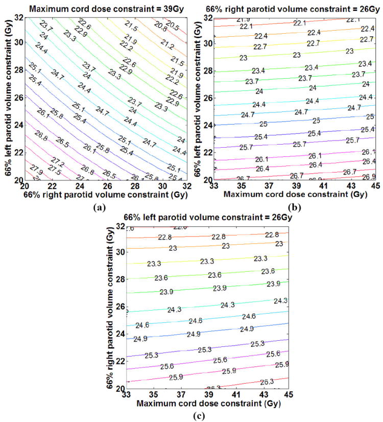
Prediction of saliva flow rate (expressed as a percentage of the pre-treatment saliva flow rate) as a function of the dose constraint settings for the three OARs: (a) fixed cord dose constraint, dose constraint ranges for LP and RP, (b) fixed RP dose constraint, dose constraint ranges for cord and LP and (c) fixed LP dose constraint, dose constraint ranges for cord and RP.

Figure 11 shows an example of the results for the prediction of Grade 2 rectal complications. The shaded region in each plot corresponds to the complication region for a range of DV constraint settings for two OARs and a fixed constraint setting for the third OAR. We attribute the unshaded region (lack of rectal bleeding) in Figure 11 (c) corresponding to increasing the bladder and bowel settings to an associated dose transfer to the bladder and bowel and reduced dose to the rectum. These results are examples of how the prediction of OAR complications can guide the selection of DV constraint settings for all OARs.

Figure 11.

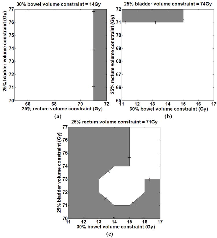
Prediction of Grade 2 rectal complications as a function of the dose constraint settings for the three OARs: (a) fixed bowel dose constraint, dose constraint ranges for bladder and rectum, (b) fixed bladder dose constraint, dose constraint ranges for rectum and bowel and (c) fixed rectum dose constraint, dose constraint ranges for bladder and bowel.

IV. DISCUSSION

The goal of this work was to investigate the feasibility of predicting OAR complications (labels) as a function of input features or DV constraint settings during the IMRT treatment planning process. Conventional IMRT treatment planning is usually an iterative process after plan generation. Planners evaluate the plan and modify the plan if the plan quality is not satisfied. Our results show that the ability to predict OAR complications as a function of DV constraint settings could guide the selection of such features corresponding to all involved OARs in the case.

Relationships between the plan DV levels and OAR complications have been established retrospectively. These data serve as the basis for formulation of dose and dose-volume constraints in IMRT inverse planning. Investigators have modeled clinical complications retrospectively using dose data in single institution and cooperative group clinical trials [24-29]. Using modeling techniques including logistic regression, multivariate analysis, support vector machines and neural networks, these investigators have successfully modeled radiation therapy related OAR complications. Our work differs from the work of these investigators in that our goal is to incorporate established dose and dose-volume parameters derived from clinical trials into the treatment planning process (prospectively). Predicting the OAR complications (labels) as a function of the DV constraint settings (features) in the planning process can guide a knowledge-driven selection of appropriate input features corresponding to all involved OARs. Incorporating the ability to predict potential complications for a given case can also allow physicians decide among rival treatment plans.

Treatment planning currently only implicitly considers treatment related complications through the evaluation of achieved dose or dose-volume levels following treatment plan optimization. The proposed clinical workflow would involve first, the creation of a collection of case-specific plans that differ in their DV constraint settings (knowledge base). Next, plan-related OAR complications would be inferred using this knowledge base and predictive algorithms described herein for any combination of features corresponding to all involved OARs. Each case would have its own unique relationship between the output labels and input features and plan properties.

With the framework developed in this work, it is possible to directly infer plan-related complications (labels) using the knowledge base of computed plans and modeling described in this work. While the work described herein has not been validated, it does present the opportunity to be validated in a clinical trial setting.

V. CONCLUSION

Our results show that using the methods described here, case-specific plan-related OAR complications can be predicted as a function of DV constraint settings. ML tools can be used to guide planners to select DV constraint settings corresponding to all involved OARs in a knowledge-driven manner.

References

- 1.Gopal R, Starkschall G. Plan space: representation of treatment plans in multidimensional space. Int J Radiat Oncol Biol Phys. 2002;53:1328–36. doi: 10.1016/s0360-3016(02)02866-3. [DOI] [PubMed] [Google Scholar]
- 2.Rosen I, Liu HH, Childress N, et al. Interactively exploring optimized treatment plans. Int J Radiat Oncol Biol Phys. 2005;61:570–82. doi: 10.1016/j.ijrobp.2004.09.022. [DOI] [PubMed] [Google Scholar]
- 3.Zhang X, Wang X, Dong L, et al. A sensitivity-guided algorithm for automated determination of IMRT objective function parameters. Med Phys. 2006;33:2935–2944. doi: 10.1118/1.2214171. [DOI] [PubMed] [Google Scholar]
- 4.Yu Y. Multiobjective decision theory for computational optimization in radiation therapy. Medical Physics. 1997;24:1445–1454. doi: 10.1118/1.598033. [DOI] [PubMed] [Google Scholar]
- 5.Xing L, Li JG, Donaldson S, et al. Optimization of importance factors in inverse planning. Phys Med Biol. 1999;44:2525–2536. doi: 10.1088/0031-9155/44/10/311. [DOI] [PubMed] [Google Scholar]
- 6.Romeijn HE, Dempsey JF, Li JG. A unifying framework for multi-criteria fluence map optimization models. Phys Med Biol. 2004;49:1991–2013. doi: 10.1088/0031-9155/49/10/011. [DOI] [PubMed] [Google Scholar]
- 7.Craft D, Halabi T, Bortfeld T. Exploration of tradeoffs in intensity-modulated radiotherapy. Phys Med Biol. 2005;50:5857–5868. doi: 10.1088/0031-9155/50/24/007. [DOI] [PubMed] [Google Scholar]
- 8.Craft D, Halabi T, Shih HA, et al. An approach for practical multiobjective IMRT treatment planning. Int J Radiat Oncol Biol Phys. 2007;69:1600–1607. doi: 10.1016/j.ijrobp.2007.08.019. [DOI] [PubMed] [Google Scholar]
- 9.Craft D, Bortfeld T. How many plans are needed in an IMRT multi-objective plan database? Phys Med Biol. 2008;53:2785–2796. doi: 10.1088/0031-9155/53/11/002. [DOI] [PubMed] [Google Scholar]
- 10.Meyer RR, Zhang HH, Goadrich L, Nazareth DP, et al. A Multi-Plan Treatment Planning Framework: A Paradigm Shift for IMRT. Int J Radiat Oncol Biol Phys. 2007;68:1178–1189. doi: 10.1016/j.ijrobp.2007.02.051. [DOI] [PubMed] [Google Scholar]
- 11.Eisbruch A, Haken RT, Kim H, et al. Glands following conformal and intensity-modulated irradiation of head and neck cancer. Int J Radiat Oncol Biol Phys. 1999;45:577–587. doi: 10.1016/s0360-3016(99)00247-3. [DOI] [PubMed] [Google Scholar]
- 12.Chao C, Deasy J, Markman J, et al. A prospective study of salivary function sparing in patients with head-and-neck cancers receiving intensity-modulated or three-dimensional radiation therapy: initial results. Int J Radiat Oncol Biol Phys. 2001;49:907–916. doi: 10.1016/s0360-3016(00)01441-3. [DOI] [PubMed] [Google Scholar]
- 13.Eisbruch A, Ship JA, Kim HM, Ten Haken RK. Partial Irradiation of the Parotid Gland. Semin Radiatnt Oncol. 2001;11:234–239. doi: 10.1053/srao.2001.23484. [DOI] [PubMed] [Google Scholar]
- 14.Jackson A. Partial Irradiation of the Rectum. Semin Radiat Oncol. 2001;11:215–223. doi: 10.1053/srao.2001.23481. [DOI] [PubMed] [Google Scholar]
- 15.Jackson A, Skwarchuk MW, Zelefsky MJ, Cowen DM, et al. Late Rectal Bleeding After Conformal Radiotherapy of Prostate Cancer (II): Volume Effects and Dose-Volume Histograms. Int J Radiat Oncol Biol Phys. 2001;49:695–698. doi: 10.1016/s0360-3016(00)01414-0. [DOI] [PubMed] [Google Scholar]
- 16.Yorke ED. Biological Indices for Evaluation and Optimization of IMRT. Intensity-Modulated Radiation Therapy: The State of the Art: AAPM Medical Physics Monograph number 29. 2003:77–114. [Google Scholar]
- 17.Fiorino C, Sanguineti G, Cozzarini C, et al. Rectal dose-volume constraints in high-dose radiotherapy of localized prostate cancer. Int J Radiat Oncol Biol Phys. 2003;57:953–962. doi: 10.1016/s0360-3016(03)00665-5. [DOI] [PubMed] [Google Scholar]
- 18.Boersma L, Van Den Brink M, Bruce A, et al. Estimation of the incidence of late bladder and rectum complications after high-dose (70-78Gy) conformal radiotherapy for prostate cancer, using dose-volume histograms. Int J Radiat Oncol Biol Phys. 1998;41:83–92. doi: 10.1016/s0360-3016(98)00037-6. [DOI] [PubMed] [Google Scholar]
- 19.Cozzarini C, Fiorino C, Ceresoli G, et al. Significant correlation between rectal DVH and late bleeding in patients treated after radical prostatectomy with conformal or conventional radiotherapy (66.6-70.2Gy) Int J Radiat Oncol Biol Phys. 2003;55:688–694. doi: 10.1016/s0360-3016(02)04117-2. [DOI] [PubMed] [Google Scholar]
- 20.Platt JC. Fast training of support vector machines using sequential minimal optimization. Advances in kernel methods: support vector learning. 1999:185–208. [Google Scholar]
- 21.Shevade SK, Keerthi SS, Bhattacharyya C, et al. Improvements to SMO Algorithm for SVM Regression. IEEE Trans on Neural Networks. 2000;11:1188–1193. doi: 10.1109/72.870050. [DOI] [PubMed] [Google Scholar]
- 22.Quinlan JR. C4.5: Programs for Machine Learning. Morgan Kaufmann Publishers; 1993. [Google Scholar]
- 23.Witten IH, Frand E. Data Mining: Practical machine learning tools and techniques. 2. Morgan Kaufmann; San Francisco: 2005. [Google Scholar]
- 24.El Naqa I, Bradley J, Blanco AI, et al. Multivariable modeling of radiotherapy outcomes, including dose-volume and clinical factors. Int J Radiat Oncol Biol Phys. 2006;64:1275–1286. doi: 10.1016/j.ijrobp.2005.11.022. [DOI] [PubMed] [Google Scholar]
- 25.Hope AJ, Lindsay PE, El Naqa I, et al. Modeling radiation pneumonitis risk with clinical, dosimetric, and spatial parameters. Int J Radiat Oncol Biol Phys. 2006;65:112–124. doi: 10.1016/j.ijrobp.2005.11.046. [DOI] [PubMed] [Google Scholar]
- 26.Bradley JD, Hope A, El Naqa I, et al. A nomogram to predict radiation pneumonitis, derived from a combined analysis of RTOG 9311 and institutional data. Int J Radiat Oncol Biol Phys. 2007;69:985–992. doi: 10.1016/j.ijrobp.2007.04.077. [DOI] [PMC free article] [PubMed] [Google Scholar]
- 27.Chen S, Zhou S, Zhang J, et al. A neural network model to predict lung radiation-induced pneumonitis. Med Phys. 2007;34:3420–3427. doi: 10.1118/1.2759601. [DOI] [PMC free article] [PubMed] [Google Scholar]
- 28.Chen S, Zhou S, Yin FF, et al. Investigation of the support vector machine algorithm to predict lung radiation-induced pneumonitis. Med Phys. 2007;34:3808–3814. doi: 10.1118/1.2776669. [DOI] [PMC free article] [PubMed] [Google Scholar]
- 29.Chen S, Zhou S, Yin FF, et al. Using patient data similarities to predict radiation pneumonitis via a self-organizing map. Phys Med Biol. 2008;53:203–216. doi: 10.1088/0031-9155/53/1/014. [DOI] [PMC free article] [PubMed] [Google Scholar]