A New Markov Random Field Segmentation Method for Breast Lesion Segmentation in MR images

Abstract

Breast cancer is a major public health problem for women in the Iran and many other parts of the world. Dynamic contrast-enhanced magnetic resonance imaging (DCE-MRI) plays a pivotal role in breast cancer care, including detection, diagnosis, and treatment monitoring. But segmentation of these images which is seriously affected by intensity inhomogeneities created by radio-frequency coils is a challenging task. Markov Random Field (MRF) is used widely in medical image segmentation especially in MR images. It is because this method can model intensity inhomogeneities occurring in these images. But this method has two critical weaknesses: Computational complexity and sensitivity of the results to the models parameters. To overcome these problems, in this paper, we present Improved-Markov Random Field (I-MRF) method for breast lesion segmentation in MR images. Unlike the conventional MRF, in the proposed approach, we don’t use the Iterative Conditional Mode (ICM) method or Simulated Annealing (SA) for class membership estimation of each pixel (lesion and non-lesion). The prior distribution of the class membership is modeled as a ratio of two conditional probability distributions in a neighborhood which is defined for each pixel: probability distribution of similar pixels and non-similar ones. Since our proposed approach don’t use an iterative method for maximizing the posterior probability, above mentioned problems are solved. Experimental results show that performance of segmentation in this approach is higher than conventional MRF in terms of accuracy, precision, and Computational complexity.

1. INTRODUCTION

Breast cancer is one of the leading causes of cancer death in Iran. The mammogram is the most effective tool in early breast cancer detection; however, it is not 100% effective. The sensitivity of the mammogram depends on density, age, and hormone status of the patients and 10-30% breast cancer are not detected. Its positive predictive value is less than 35%[1]. Hence we need to use other imaging modality such as MRI[2]. The MRI modality is used simultaneity as an appropriate scenario with mammography, especially for women at high risk. Some studies have shown that MRI is superior to x-ray mammography and sonography in order to determine breast cancer tumor volume[3–5].

Several segmentation techniques are presented in the literature[6,7] such as Region-based segmentation techniques[8,10] contour-based segmentation[11,12] and classification-based segmentation methods including supervised and unsupervised algorithms[13–17]

Among the many existing segmentation methods, the accurate segmentation of MR images seems a challenging task. One of the important persistent difficulties is the spatial inhomogeneity of the MR signal with which many methods at the present deal. The Markov Random Fields have been used in many image processing problems including image restoration and segmentation[18–20].

Since Markov Random Field models spatial interaction between neighboring pixels, it can overcome spatial inhomogeneity in MR images. Hence it is used widely in medical image segmentation. But this method has also some weakness: Computational complexity and sensitivity of the results to the models parameters. In order to address these difficulties, we have developed a new Markov Random Filed (I-MRF) segmentation method.

This proposed method doesn’t need an image with primary labels and never used the iterative methods such as SA or ICM to maximize posterior probability. For these reasons, the computational complexity of algorithm is reduced. We also use texture features to measure the similarity between pixels in this paper, because textures are one of the most important image attributes and can distinguish the objects with different patterns. Gibbs et al.[21] used texture analysis in diagnosis of benign and malignant breast lesions.

This paper is organized in different parts and sections. : In section 2; we introduce conventional MRF and Finite Gaussian Mixture, the proposed algorithm will be explained in section 3, section 4 investigate the experimental results of our approach and compare them with by conventional MRF, and finally; discussion and conclusion comes in section 5.

2. METHODS

A. Image Dataset

In this paper, we used the PIDER Breast MRI dataset (https://imaging.nci.nih.gov/ncia). This dataset includes breast MRI images from 5 patients and their Ground Truth (GT) segmentation that have been identified by a radiologist manually. GT is used as a reference for performance evaluation of segmentation methods in our experiments.

B. ROI selection

Since Automatic segmentation of medical images is a challenging task and still unsolved problem for many applications, and also experience of a radiologist can increase performance of algorithm, we present an interactive segmentation approach according to the identified region of interest (ROI). In our approach, at first an experienced radiologist examines and draws ROIs on MR image data with the help of image analysis software, and then we give these ROIs as an input image to algorithm.

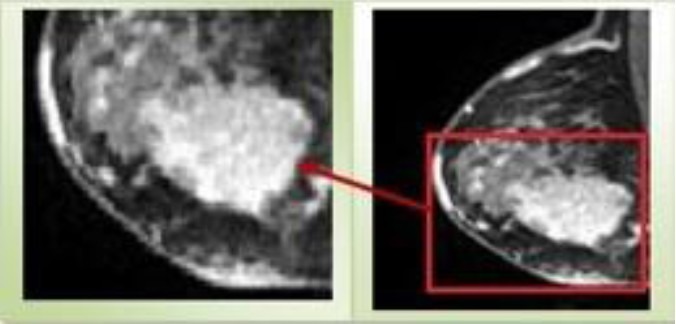
Since The ROI is defined by placing a box whit limited size (that completely contains the region of breast lesion), the segmentation complexity is reduced. A sample of ROI is shown in Figure 1.

Figure 1.

Region of Interest

C. The FGM and the MRF Models

Markov random field (MRF) model is not a segmentation method in itself, but it is a statistical model, which can be used for segmentation methods. It works with the fact that a pixel belongs to the class in which the neighbors’ pixels. It means that the probability of selecting an outlying pixel is very low. MRF provides an approach to model the variety of image properties and often works with clustering segmentation such as K-means algorithm under a Bayesian prior model[22–25]. It segments the images by maximizing the posterior probability with the help of the ICM[26] or SA[27]. For a better understanding the Markov Random Field model, we defined the Finite Gaussian Mixture (FGM) at first.

In statics, A Gaussian mixture model is a probabilistic model that assumes all the data points are generated from a mixture of a finite number of Gaussian distributions with unknown parameters. Suppose X = {x₁, x₂ …, x_N} is a random observation data set. x_i is a d-dimensional random variable. p_i(x|θ_i is the corresponding probability density function, in witch x∈ R^d is the value of x_i and θ_i is the parameter.

In segmentation application, the FGM assumes that the entire image can be expressed as overlaps of Gaussian distributions of its features. The FGM parameters are learned by sequentially applying the Expectation Maximization (EM) algorithm.

Suppose that x_i is the observed intensity of pixel. And let L, I and γ denote the sets of tissue class L= {lesion, non-lesion}, pixel index I = {1,2, ..., N}, and model parameters γ = {θ_l| l∈L} respectively. For every l ∈ L and i ∈ I,

l_i ∈ L      (1)

P(x_i|l) = ƒ(x_i; θ_l      (2)

Finite Gaussian Model is defined by mean μ_l and variance σ_l as follows:

It is a mathematically simple model and can be computed efficiently. But one of the limitations is not considering spatial information. This method only uses the intensity histogram for segmentation, and therefore, it is sensitive to noise and other artifacts. The Markov Random Field is proposed to overcome this weakness[28].

MRF adds the term P(l) to Equation 3, and solves the segmentation problem with maximizing the Equation 4. P(l) Indicates the prior probability distribution of class tissue l.

In other words, the only difference between FGM and MRF model lies in whether the spatial constraint is encoded. To estimate the P(l), based on the Hammersley-Clifford[29] theorem we can write:

Where Z is a normalizing constant, U(x) is the energy function, and V_c denotes a clique potential.

3. PROPOSED APPROACH

Although MRF models have provided better results by taking into account the spatial relationship between neighboring pixels, its computation overhead is much larger than the FGM and other method segmentation[30]. This can be easily understood because the MRF model uses an iterative optimization method such as SA or ICM to find appropriate distribution of labels.

In this new method, we apply the ratio of two conditional probability distributions to estimate the prior distribution. Hereby, we eliminate the need to use iterative method that lead to high computational complexity.

In this new method, we apply the ratio of two conditional probability distributions to estimate the prior distribution. In this way, the essentiality of using a repetitive method, which causes to enhance the complexity of computation, is omitted.

As mentioned in section2, a MRF model can be defined as:

l^* = ^argMax_l∈L(P(l|x_i) = P(x_i|l)P(l))      (4)

If we define D_i as a neighborhood for each pixel x_i, then the Equation 4 can be rewritten as follow:

l^* = ^argMax_l∈L(P(l|x_i) = P(x_i|l, D_i)P(l|D_i))      (6)

According to γ, we can use Bayes’ formula to write:

P(l|D_i) ≈ P(θ_l|D_i)      (7)

The main idea of the MRF model is that a pixel is more likely to be of a certain tissue type if the neighboring pixels are also of the same type. Based on this assumption, we use Equation 8 instead of Equation 5 to estimate the prior distribution P(θ_l|D_i).

P(θ_l|D_i) = P(D_similar|θ_l)/P(D_{non–similar}|θ_l)      (8)

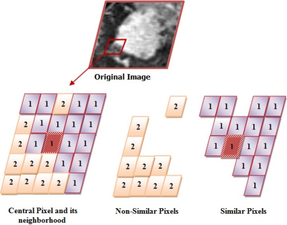
Where D_similar and D_{non–similar} are the sets of similar and non-similar pixels to the x_i respectively.

If we assume that the pixels are independent, then term P(D_similar|θ_l) can be calculated as follows:

P(D_similar|θ_l) = Π_j^{similar–length} x_j      (9)

These sets are represented by a simple graphical model in Figure 2.

Figure 2.

similar and non-similar sets

According to the main assumption in MRF, when conditional probability P(D_similar|θ_l) has a high value in Equation 8, the posterior probability of tissue l is maximized. In this method, we also use potential information of non-similar pixels by P(D_{non–similar}|θ_l).

To estimate the P(D_similar|θ_l) and P(D_{non–similar}|θ_l) in Equation 8, we need to create the sets of D_similarand D_{non–similar}. Many of the presented methods in breast lesion segmentation used only the intensity value as a feature for each pixel, which is subject to image noise, patient motion, and MR artifacts[31–32].

A. Similarity measure

On the other hand, since textures are one of the most important characteristics of an image, and also radiologists rely on textures to make diagnostic decisions, Features extraction basis from texture is most widely used in medical image processing[33]. Texture feature attempts to identify gray level variations between adjacent pixels in the image[34].

In this paper, we use three categories of texture feature: First order statistical parameters based on histogram, second order statistical parameters based on Co-occurrence, and Run-Length matrixes. For each pixel in the region of interest, we used a block 5*5 whose feature values are assigned to central pixel of block. Histogram statistics (six features) describes the intensity distribution within the block such as mean and standard deviation. The equation of these texture features are listed in appendix.

Co-occurrence matrices[35] which measure the joint probability of two adjacent Pixels along a given direction with co-occurring values i and j are calculated for 0°, 45°, 90°, and 145°. An average co-occurrence matrix is then computed for each texture block since no directional variations in texture are expected. We calculate 22 features form Co-occurrence matrices that measure joint probability of two nearest pixels in four directions.

The run-length matrix masseurs the abrasiveness of a texture in a given direction θ. Direction is the number of runs of pixels with a gray-level and a run length. A gray-level run is defined as a set of consecutive pixels with the same gray value in the given direction[36]. 11 features obtained from Run-Length matrix for same direction θ= 0°, 45°, 90°, and 145°. Totally, we extracted 39 texture features for each pixel.

After extracting the features for each pixel, we use Equation 10 to determine similarity between central pixel and their neighboring pixels. In this Equation the pixel i is similar to j, when h_i,j ≥ 0.61.

σ², Indicates the variance of pixel values in D and d_i,j is Euclidean distance between pixel i ,j.

4. EXPRIMENTAL RESULT

In this section, the performance of proposed method is investigated using PIDER Breast MRI dataset (https://imaging.nci.nih.gov/ncia). This dataset includes breast MRI images and their Ground Truth (GT) segmentation that have been identified by a radiologist manually.

GT is used as a reference for performance evaluation of segmentation methods in our experiments. 16 breast images from dataset are used as the test images. Due to space limitation, we only show the result of 5 images out of 16 test images in separate Tables. The ROIs of these images and their GTs have been shown in two first rows of Table 6. Finally the result of the all 16 test images is demonstrated in Table 5.

Table 6.

SEGMENTATION RESULTS FOR CONVENTIONAL MRF AND PROPOSED METHOD

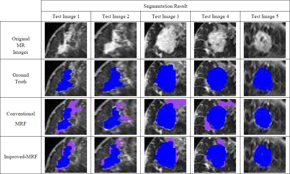
TABLE 5.

SEGMENTATION RESULTS FOR CONVENTIONAL MRF AND PROPOSED METHOD (ALL 16 TEST IMAGES)

B. Evaluation criteria

Many different measures for evaluating the performance of an algorithm have been proposed such as volume overlap ratio, specificity, sensitivity, precision, accuracy, and etc. First, we give a definition of some expressions in Table 1.

TABLE 1.

DEFINITION OF SOME EXPRESSIONS

1. Accuracy

This criterion is used to measure the similarity between assigned labels by computer algorithm and real labels given by a radiologist.

2. Precision

Unlike accuracy, precision criterion is used to measure reproducibility or repeatability of assigning a label in the same condition.

3. Specificity

This criterion measures the proportion of negatives which are correctly identified.

4. Sensitivity

This criterion measures the proportion of actual positives which are correctly identified. These two latest measures are closely related to the concepts of errors.

5. Volume overlap ratio

In this study, we also use the overlap ratio to quantify how well the computer results and the radiologist's delineation agrees. If P_c denote the set of lesion pixels which is came from the computer algorithm result and P_r denote the set of lesion pixels which is came from the radiologist's segmentation, the volume overlap ratio (VOR) is defined as:

In which the ∩ operator is logical AND, ∪ is the logical OR. It takes value between [0 1], when it is zero. It means that there is no overlap, and one means the exact overlap[37].

6. Computational complexity

The Computational complexity criterion is used to measure the time required to implement each of the algorithms for segmentation an image.

The segmentation methods described in this paper is numerically implemented using Matlab 7.9 (R 2009b).

7. Other Criterion

We also describe the accuracy with other parameters: True Positive Volume Fraction (TPVF), True Negative Volume Fraction (TNVF), false positive volume fraction (FPVF), and false negative volume fraction (FNVF). These parameters are defined as follows[38]:

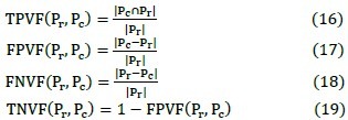
We just use the two of these volume fractions and the sum of them; TPVF and TNVF.

C. Performance evaluation for conventional MRF

We performed several kinds of experiments. At first, we evaluate the performance of conventional MRF in breast MRI image segmentation. In this section, we used SA algorithm to maximize the a posterior probability. Since the initialization has a significant impact on rapidly of the convergence of the SA procedure and on the quality of the final estimates, a Thresholding method has been used for this purpose.

As it is evident in Table 3 and 5, MRF has provided good segmentation results by 4000 iterations, but its computing time is very high.

TABLE 3.

SEGMENTATION RESULTS FOR CONVENTIONAL MRF

The segmentation results of Conventional MRF have been shown in the row 3 of Table 6.

D. Performance evaluation for Improved-MRF

Before doing the experiments to investigate proposed method, to determine the appropriate size of neighborhood, some analyses were down. First we defined the neighborhood with different size of 3,5 …27. Afterward, the sum of two volume fractions (TPVF+ TNVF) and computing time were calculated for proposed approach in each neighboring size.

Figure 3 and 4 shows the results of experiment. The computing time and volume fractions of presented method are increased by the growing of neighborhood size. As is clear, the neighborhood with size 21*21, provides a proper balance between time and sum of (TPVF+ TNVF). For these reason we used this size of neighborhood to evaluate our method.

Figure 3.

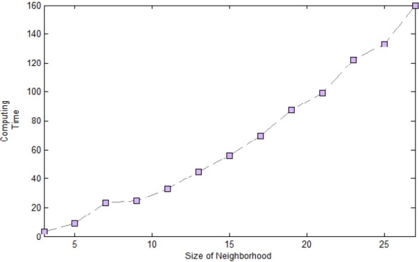
Complexity of Algorithm In Different Size Of Neighborhood

Figure 4.

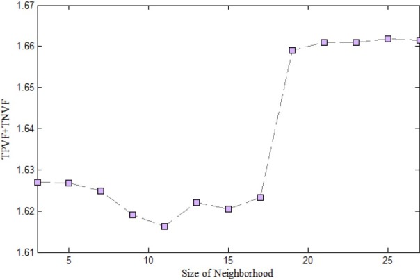
sum of two volume fraction TPVF and TNVF in each size of Neighborhood

According to Table 4 and 5 the results of I-MRF are much better than conventional MRF in terms of accuracy and computing Time. The segmentation results of Conventional MRF have been shown in the row 4 of Table 6.

TABLE 4.

SEGMENTATION RESULTS FOR IMPROVED-MRF

To evaluate the performance of the classifiers, Receiver operating characteristic (ROC) analysis also is performed. ROC is based on statistical decision theory and it has been applied widely to the evaluation of clinical performance. The area under the ROC curve is referred index. It is used as a measure of the classification performance. A higher A_Z indicates better classification performance because a larger value of True Positive (TP) is achieved at each value of False Positive (FP). The value of A_Z is 1.0 when the diagnostic detection has perfect performance, which means that TP rate is 100% and FP rate is 0%. The values of A_Z have been shown in Table 2.

TABLE 2.

THE VALUES OF A_Z

The ROC diagram is shown in the Figure 5.

Figure 5.

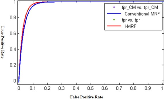
ROC curve for Supervised and IMPST methods

5. CONCLUSION AND DISCUSSION

Markov Random field approaches are widely studied for medical image segmentation, especially in MR images. It is because this method can model intensity inhomogeneities occurring in these images. But this method has two critical weaknesses: Computational complexity and sensitivity of the results to the models parameters. To overcome these problems, in this paper, we propose a new Markov Random Filed method for breast lesion segmentation in MR images and illustrate its effectiveness.

This approach can produce better results compared to conventional MRF, in terms of accuracy and computing time because:

• 1-In conventional MRF, the energy function is calculated only based on the labels of neighboring pixels that assigned randomly. But in our approach labeling each pixel is performed with high accuracy due to better characterization of neighborhoods.
• 2-Although MRF models have provided good results by taking into account the spatial relationship between neighboring pixels, but its complexity is very high. The Improved-MRF eliminates the need to use iterative method and initializing that lead to high computational complexity.

Also we believe that the idea of using the ratio of two probability distribution of similar and non-similar pixels in a neighborhood may be contributive to other application such as Microcalcification segmentation in breast MR images, as well. In addition, The factor that influences the performance of proposed algorithm is the simple policy that has been used to determine similarity between central pixel and their neighboring pixels (Equation (10)).in fact we used an empirical threshold. If we use the better and more sophisticated policy in order to determine similarity between pixels, definitely we will get better results. In future work we intend to use the Gossip protocol for this purpose.

6. APPENDIX

The list of three categories (First order statistical parameters based on histogram, second order statistical parameters based on co-occurrence matrix, Run-Length Matrix) textural features have been used in this paper is given as follows:

Statistic:

1. Mean

2. Skewness

3. Absolute Deviation

4. Variance

5. Kurtosis

6. Standard Deviation

Co-occurrence Matrix:

Notation:

p(i,j): (i,j)-th entry in a normalized gray-tone spatial-dependence matrix.

p_x(i): is the i-th entry in the marginal-probability matrix obtained by summing the rows of p(i,j),=Σ^N_j=1p(i,j)

N: is the number of distinct gray levels in the equalized image.

1. Uniformity / Energy / Angular Second Moment:

   ƒ₁ = Σ_iΣ_i(_i,_j)²

2. Contrast/Inertia:

   

3. Correlation

   

4. Variance:

   ƒ₄ = Σ_i(i–μ_x)²P_x(i)

5. Homogeneity/Inverse difference moment

   

6. Sum Average

   ƒ₆ = Σ^2N_n=2nP_x+y(n)

7. Sum Variance

   

8. Sum Entropy

   

9. Entropy

   

10. Difference variance

    ƒ₁₀ = Σ^N–1_n=0(n–μ_x–y)²P_x–y(n)

    Where μ_x–y is the mean of P_x–y

    Where μ_x and σ_x are the mean and standard deviations P_x, Respectively.

11. Difference entropy

    

12. Information measures of correlation (1)

    

13. Information measures of correlation (2)

    

    Where H_xy = -Σ_iΣ_jP(i,j)log (P_x(i)P_x(j))

14. Maximal correlation coefficient

    

    Where Q(i,j) = Σ_k(P(i,k)P(j,k))/(P_x(i)P_x(k)).

15. Autocorrelation

16. Cluster Shade

17. Cluster Prominence

18. Maximum probability

19. Sum of Squares

20. Inverse difference

21. Inverse difference normalized (INN)

22. Inverse difference moment normalized (IDN)

Run-Length Matrix:

1. Short run emphasis:

   

2. Long run emphasis:

   

3. Gray level nonuniformity :

   

4. Run-length nonuniformity :

   

5. Run Percentage (RP)

   

6. Low Gray-Level Run Emphasis (LGRE):

   

7. High Gray-Level Run Emphasis (HGRE)

   

8. Short Run Low Gray-Level Emphasis (SRLGE)

   

9. Short Run High Gray-Level Emphasis (SRHGE)

   

10. Long Run Low Gray-Level Emphasis (LRLGE)

    

11. Long Run High Gray-Level Emphasis (LRHGE):

    

Nomenclature of Symbols and Acronym:

DCE-MRI : Dynamic contrast-enhanced magnetic resonance imaging

MRF: Markov Random Field

I-MRF: Improved-Markov Random Field

ICM: Iterative Conditional Mode

SA: Simulated Annealing

FGM: Finite Gaussian Mixture

GT: Ground Truth

TP: True positive

FP: False positive

FN: False negative

TN: True negative

VOR: volume overlap ratio

TPVF: Positive Volume Fraction

TNVF: True Negative Volume Fraction

FPVF: false positive volume fraction

FNVF: false negative volume fraction

ROC: Receiver operating characteristic

L: set of tissue type

I : set of pixel index

γ: set of Model Parameters

P(x_i|l) : Probability distribution function

P (l) : Prior probability distribution

Z : normalizing constant

U(x) : Energy function

V_c : A clique potential

θ_l : Model parameters for tissue l

μ : Mean

σ : Variance

x : Random variable

D_i : A neighborhood for each pixel x_i

D_similar : set of similar pixels to the pixel x_i

D_{non–similar}: set of non-similar pixels to the pixel x_i

d_i,j : Euclidean distance between pixel i ,j

∩: Logical AND

∪: Logical OR

A_Z: area under the ROC curve