Automatic Detection of Pectoral Muscle Using Average Gradient and Shape Based Feature

Abstract

In medio-lateral oblique view of mammogram, pectoral muscle may sometimes affect the detection of breast cancer due to their similar characteristics with abnormal tissues. As a result pectoral muscle should be handled separately while detecting the breast cancer. In this paper, a novel approach for the detection of pectoral muscle using average gradient- and shape-based feature is proposed. The process first approximates the pectoral muscle boundary as a straight line using average gradient-, position-, and shape-based features of the pectoral muscle. Straight line is then tuned to a smooth curve which represents the pectoral margin more accurately. Finally, an enclosed region is generated which represents the pectoral muscle as a segmentation mask. The main advantage of the method is its’ simplicity as well as accuracy. The method is applied on 200 mammographic images consisting 80 randomly selected scanned film images from Mammographic Image Analysis Society (mini-MIAS) database, 80 direct radiography (DR) images, and 40 computed radiography (CR) images from local database. The performance is evaluated based upon the false positive (FP), false negative (FN) pixel percentage, and mean distance closest point (MDCP). Taking all the images into consideration, the average FP and FN pixel percentages are 4.22%, 3.93%, 18.81%, and 6.71%, 6.28%, 5.12% for mini-MIAS, DR, and CR images, respectively. Obtained MDCP values for the same set of database are 3.34, 3.33, and 10.41 respectively. The method is also compared with two well-known pectoral muscle detection techniques and in most of the cases, it outperforms the other two approaches.

Introduction

Cancer is the second (after heart disease) and third (following heart and diarrhoeal diseases) leading cause of death in economically developed countries and in developing countries, respectively [1]. According to American cancer society [1], in 2007, worldwide new breast cancer cases were 1,301,867 (women), and deaths due to this disease were 464,854. In 2011, in the USA, estimated new breast cancer cases are 230,480 and estimated deaths due to this disease are 39,520 among women [2].

Early detection can prevent breast cancer and X-ray mammography is the most effective clinical choice for early detection [1]. For automatic identification of breast cancer from mammogram, pectoral muscle plays an important role in a negative sense. Normally, in medio-lateral oblique (MLO) view of mammogram, pectoral muscle appears as a triangular, high-density region at the posterior corner of the image. The presence of pectoral muscle can affect the automatic detection of suspicious regions such as mass [3, 4], or automatic identification of breast tissue density [5, 6]; as the pectoral muscle approximately have the same density, so is the dense tissues of interest in the image.

In recent past, several works were proposed on automatic identification of pectoral muscle. Some papers used straight line to fit the pectoral muscle boundary. Such as Karssemeijer [5] and Ferrari et al. [7] used Hough transform and Kinoshita et al. [8] applied Radon transformation to approximate pectoral edge by a straight line. These types of straight line representation may create massive error when the pectoral muscle boundary is curve. Yam et al. [9] tried to solve this problem by refining the straight line obtained by Hough transform into a curved pectoral edge using dynamic programming. In 2004, Ferrari et al. [10] employed an efficient detection algorithm based on Gabor wavelet to obtain a smooth pectoral edge. Use of 48 Gabor filters with 12 orientations and 4 scales to detect edge points is a very time-consuming method. Kwok et al. [11] in their work used an iterative thresholding method to detect pectoral muscle approximately and then applied a gradient-based searching on the roughly obtained edge to find the final boundary points. Two graph-based detection methods were realized by Bajger et al. [12] and Ma et al. [13]. A discrete time Markov chain was applied by Wang et al. [14] for rough pectoral muscle boundary detection and an active contour model for refining it.

The aim of the proposed work is to develop a new technique for the detection of pectoral muscle, in MLO view of the mammographic image, more accurately than the existing techniques, in terms of low false positive and false negative rates. The technique does not consider the craniocaudal (CC) views, since only 30–40% CC view images contain pectoral muscle [15]. The proposed method first approximates the boundary by a straight line. Within a selected region, maximum discontinuity points are determined along each horizontal line, based upon the weighted average gradient. An adaptive shape-based method is then applied to divide these points into a number of bands. The band with maximum number of points is considered as the most probable band containing probable pectoral edge points. A straight line is then estimated based upon the probable pectoral edge points. To determine pectoral muscle boundary more accurately, obtained straight line is then fine tuned to a smooth curve by taking a small region around the line and finding out more accurate points. The final segmented pectoral muscle region is assessed by one radiologist and compared with two well-known pectoral muscle detection algorithms.

The remaining paper is organized as follows: “Method” section discusses the method used for detection of pectoral muscle. Experimental setup and evaluation metrics for performance analysis are presented in “Experimental Setup and Evaluation Metrics”. The next section is the “Results and Discussion” section. Conclusions are drawn in the “Conclusion” section.

Method

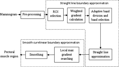
This section describes the method used to detect pectoral muscle. Steps of which are given in Fig. 1. Basic building block of the algorithm is based on the following characteristics of pectoral muscle.

Fig. 1.

Block diagram of proposed pectoral muscle detection technique

Pectoral Muscle Characteristics

1. It is a high-intensity region than the surrounding background.

2. At the edge of the pectoral muscle, there is a sharp change in intensity.

3. Pectoral muscle is roughly triangular in shape.

4. It is visible in the upper posterior position of the MLO view of the breast image.

5. Two edges of pectoral muscle are the part of breast image boundary.

Before the detection step, image is preprocessed for orientation fixing, and breast border extraction. For simplicity of the algorithm, the mammographic image is oriented in such a way that the pectoral muscle is located at the top-left corner of the image, i.e., the right breast image is mirrored vertically and if required, image is shifted. Then the breast region segmentation is executed automatically by using SBS method [16].

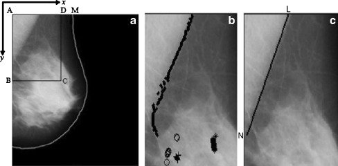
As the two edges of pectoral muscle are part of image boundary (top and left boundary), it is only required to find out the third edge which cut the other two boundaries and forms approximately a triangular shape (Fig. 2a). At the first step of detection, the third edge is approximated by a straight line. A region of interest (ROI) is selected which may not always contain whole pectoral muscle region, but is adequate to find out a straight line representing the approximate pectoral muscle boundary. The straight line approximation creates immense error when pectoral muscle boundary is a curve. After the first step of straight line approximation, obtained straight line is fine-tuned to a smooth curve to represent the pectoral muscle boundary more accurately, by searching maximum gradient points within a limited band around the approximated boundary.

Fig. 2.

a Original mammogram image mdb001 from mini-MIAS database, with region of interest ABCD, after breast region segmentation and orientation fixing; b ROI with band of maximum gradient pixels, different symbols represent different band; cstraight line approximation of the pectoral muscle

Straight Line Approximation

1. ROI selection: In this method, the top-left point of the image is considered as the origin of the image coordinate system and horizontal and vertical directions are defined as x- and y-axis, respectively (Fig. 2a). A rectangular area (ABCD) is selected as an ROI as shown in Fig. 2a, where A (0,0), top-left pixel on the breast boundary, B (0,y_e), middle point between top-left and bottom-left point, D(x_e,0) top-right point which covers 80% of the top-breast boundary (AM), and C (x_e,y_e) that completes rectangle with A, B, and D.

2. Weighted average gradient calculation: Pectoral muscle is generally a high-intensity region with sharp intensity change at the boundary. To detect edge points of the pectoral muscle, a weighted average gradient is proposed here. For each point within the ROI, average gradient is calculated by taking average of intensity differences along x-axis, which can be defined as,

   1

   where, (x, y) = coordinate of the pixel where gradient is calculated,

   N

   number of pixel pairs used for average gradient computation

   I(x, y)

   intensity of the pixel at (x, y) position.

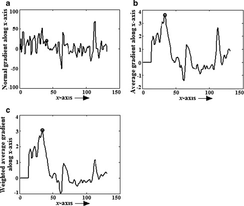
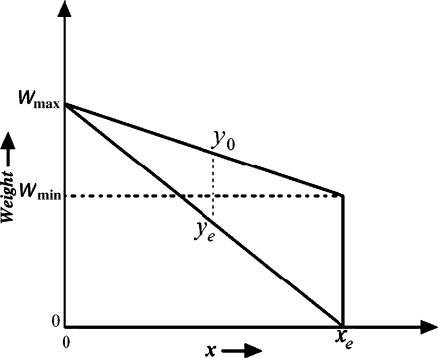
   Use of average gradient reduces the effect of high intensity variation of noise spike and curvilinear structure as shown in Fig. 3. Sometime, right side breast boundary, glandular tissues, and mass in ROI may have high average gradient. To suppress them and emphasize pectoral muscle, a weight function is introduced. For the orientation fixing, pectoral muscle is always closer to the left boundary of the breast than the right boundary and the third edge can be considered as a decreasing function of y. So, to highlight desired edge points, a monotonically decreasing function of both x and y is chosen as weight function (Fig. 4), which can be represented by,

   2

   where, w_min(y) = weight at (x_e, y) and w_max(y) = weight at (0, y) here, w_max(y) = W_max,

   

3. Division of maximum gradient points into bands: Generally, maximum-weighted gradient point on each horizontal line should be the member of pectoral muscle boundary. But due to artifacts and noisy effects some points may not represent edge points, though most of them characterize pectoral muscle boundary which are sufficient for the straight line approximation. Due to the noisy edge points, line drawn using least square error criterion is not always successful. Use of RANdom SAmple Consensus method may help to eliminate the noisy edge points but being iterative in nature the processing is computation intensive and slow. To find those desired points, all maximum gradient points are then divided into a number of bands. Pectoral muscle edge points maintain a particular arrangement. Successive points on the edge are close to each other and the edge curve is right-slanted. So, the edge can be considered as a function of y with an overall negative slope, though in small part of the edge it may have positive or zero slopes. Bands are formed in such a way that elements of a band conform to these constrains. Process starts from top to bottom. Initially, the maximum gradient point on the topmost horizontal axis (y = 0) forms the first element of the first band. Then successive points are checked. At each horizontal line, expected position of the band is estimated. As, in a small region edge can be considered as a straight line, expected next position is calculated using the average rate of change of previous positions (n points) within the band. If the next point is within a small range (δ) of expected value, it is considered as a point of same band otherwise a new band is created. The process is followed for all the probable edge points. After checking the range criteria for each band, the pectoral edge pixel is added to all the bands where the criterion is satisfied. In this way, maximum gradient points are divided into a number of bands as shown in Fig. 2b. Algorithm for the aforementioned band division technique is given below:

4. Selection of bands: Band with maximum points is selected as the most probable band.

5. Straight line approximation: Straight line fitting using least square error is then applied and straight line approximation (LN) is found out for the pectoral muscle boundary as shown in Fig. 2c.

Fig. 3.

For mdb001, y = 144, gradient along x-axis, a normal gradient using Sobel operator, b average gradient with N = 10, c weighted average gradient with N = 10, W_max = 1 and W_min = 1/4

Fig. 4.

Weight function

Smooth Boundary Detection

1. Local gradient search: A local edge searching process is proposed for refining the boundary. The basic idea of this step is similar to [11]. At each point on LN, a perpendicular line segment, equal in both side (say d), is defined for searching the edge point. The points for which part of the search line segment stretched beyond the breast region is rotated to accommodate the search line within the breast image boundary (Fig. 5a). In the proposed searching method, edge points are determined by calculating average gradient along each search line and finding out maximum gradient point. In comparison, Kwok et al. [11] used a sigmoid function to represent the intensity profile of points on search line and considered inflection point as an edge point. Sometime, it is observed that the lower part of the pectoral muscle deviate from the straight line. In those cases, searching over a constant search path around the straight line may not contain the original edge point. To avoid this, instead of fixing the reference point on the straight line, we have added some flexibility to change that reference point. An expected position of the edge point is calculated for the next row, based on the average rate of change of the previous rows. If the expected position belongs outside the search line segment, line segment is shifted in such a way that it covers the expected position. This dynamic adjustment of search line increase chances of detection of true edge points (Fig. 6).

2. Remove and fill points along y-axis: For each point on LN (Fig. 5a), the search for maximum average gradient is conducted along the perpendicular line. In this process, for each row (y-position), the number of detected pectoral edge pixel could be 0, 1 or more than 1. If more than 1 pectoral edge pixel is detected in a row, the point having maximum gradient value is chosen. For no edge pixel in a row, the pectoral edge pixel is estimated by linear interpolation at the adjacent edge points (Fig. 5b).

3. Trimming of phantom pectoral edge: If the pectoral muscle region ends before the approximated straight line, the local searching gives rise to some extra points, which are called as phantom edge points. To remove these points, we find the first edge point which is close to the left boundary (within β1) of the breast image. This may be the end point or noisy point. To check whether points following this one are real edge point; mean intensity of the row within pectoral muscle edge is calculated. If the computed mean intensity deviate far from the upper part of pectoral muscle, it is clear that this is a phantom pectoral edge. Phantom pectoral edge beyond the end point is deleted.

4. Smoothing: To smooth the boundary obtained in the previous step, two-step averaging is applied in this method. First, a moving window averaging filter is selectively applied. Edge pixels which deviate much from the average value within a window are only replaced by the average. This selective averaging is used to avoid the effect of noisy points on accurate points while averaging. After selective averaging, the same averaging filter is applied to smooth the obtained edge curve.

5. Region closing: After moving average filter with kernel length 2w + 1, we have w points left at both the ends without filtering. These points are replaced by extrapolating the line using local gradient.

Fig. 5.

Smooth boundary detection steps, a mdb001 with perpendicular search path on which maximum gradient is calculated, b pectoral edge after local gradient search and removal and fill up steps, c edge after selective averaging, d edge after final smoothing and region closing

Fig. 6.

Dynamic adjustment of search line while expected position is outside the reference search line segment

Experimental Setup and Evaluation Metrics

Database

To test the algorithm, three different types of database are used

1. Scanned film images: The experiment was conducted on 80 images of the Mammographic Image Analysis Society, London, UK (mini-MIAS). All the images are MLO views with 200 μm sampling interval and 8 bit gray-level quantization. The images were down sampled by a factor of 2 for reduction of processing time, which changed the size from 1,024 × 1,024 pixels to 512 × 512 pixels and pixel resolution to 400 μm.

2. Direct radiography images (DR): DR images are collected from local medical institute, which maintain 70 μm sampling interval and 12 bit gray-level quantization. All the images were first anonymized and a total of 80 MLO view images were taken for the experiment. The images were reduced in size by a factor of 8 in each dimension, which transform the size from 2,560 × 3,328 to 320 × 416 and pixel resolution to 560 μm.

3. Computed radiography images (CR): CR images are also collected from a local institute. These images are of 4 megapixels (spatial resolution 1792 × 2,392) with 12-bit intensity resolution and pixel resolution of 97 μm. A total of 40 images were taken for this experiment. They were anonymized first and then reduced by a factor of 4 in each dimension (converted size = 448 × 598 and pixel resolution = 388 μm).

Experimental Setup

The algorithm is implemented in Matlab 7.9 version on Intel Core Duo processor having operating system windows XP, frequency 2.80 GHz and memory of 1.98 GB. Performance of the method is measured for all the aforementioned database. The key parameters are selected by analyzing the images as well as by verifying it experimentally. It is observed that average gradient gives better result than normal gradient operators (viz. Sobel). But number of pixel pairs on which gradient will be averaged should not be so high that it suffers from the effect of dense glandular tissues of breast region. In the experiment, N in Eq. 1 is kept as 10 pixels. In the band division, algorithm tolerance δ₁ and δ₂ are introduced. Any small positive integer in the range [3–12] and [1–5] may be used for them. Small variations of these parameter values do not affect the performance. In the present work, δ₁ and δ₂ are taken as10 and 5, respectively.

Reference pectoral muscle edges are drawn manually by one of the author in consultation with an experienced radiologist. Before this, contrast and brightness of images were enhanced manually by using Adobe Photoshop to visualize edges more prominently.

Performance Metrics

To evaluate the proposed method, the following five performance metrics were used:

1. False positive (FP) pixel percentage: FP pixel can be defined as the pixels inside the obtained pectoral muscle boundary but outside the reference pectoral muscle boundary. Mathematically, false positive pixel percentage can be defined as,

   

   where,

   A

   {(x,y) ∈ obtained pectoral muscle region}

   B

   {(x, y) ∈ reference pectoral muscle region}

2. False negative (FN) pixel percentage: the pixels inside the reference pectoral muscle boundary but outside the obtained pectoral muscle boundary normalized by the total pixel of the reference pectoral muscle region.

3. Total mismatched pixel percentage: It is obtained from FP and FN pixels and can be defined as,

4. Hausdorff distance: It is defined as,

   

   where,

   C

   {(x, y) ∈ reference pectoral muscle boundary points}

   D

   {(x, y) ∈ obtained pectoral muscle boundary points}

5. Mean distance closest point (MDCP): MDCP is another metric used to evaluate the closeness between the reference edge and obtained edge,

   

Results and Discussion

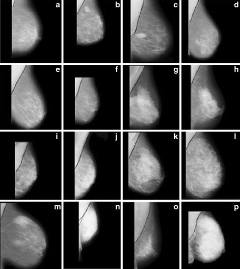
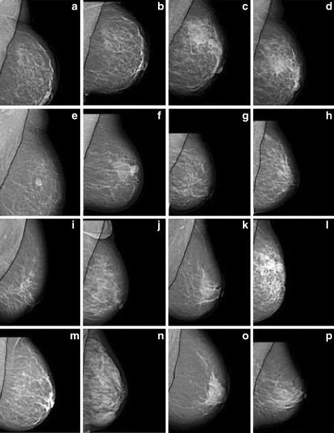
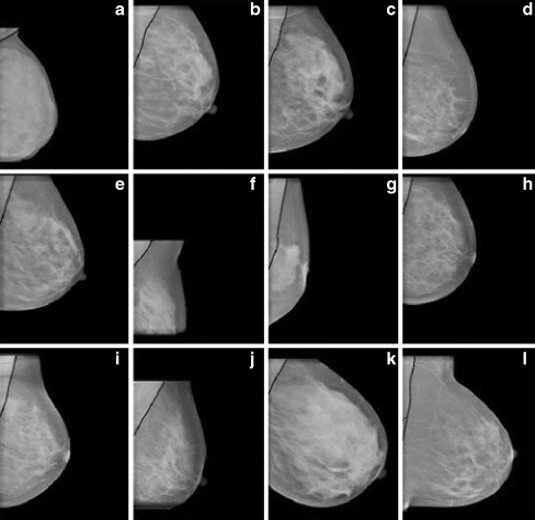
The proposed algorithm is applied on three different types of database. To evaluate the efficiency of this method, previously mentioned performance evaluation metrics are used. Some of the results are shown in Figs. 7, 8, and 9. The proposed method is compared with two well-known pectoral muscle detection algorithm proposed by Ferrari et al. [10] and Kwok et al. [11]. Till now, these are the best among the methods reported in literature to detect pectoral muscle. Both these methods were implemented on the same platform. If any one of the FP pixel percentage or FN pixel percentage is greater than 30%, we consider that the detection has failed. Tables 1, 2, and 3 summarizes the comparative results of all these methods for mini-MIAS database, DR images, and CR images, respectively.

Fig. 7.

Segmentation results obtained by the proposed pectoral muscle detection algorithm for some mini-MIAS images a mdb013, b mdb015, c mdb025, d mdb058, e mdb059, f mdb080, g mdb110, h mdb121, i mdb123, j mdb124, k mdb125, l mdb130, m mdb150, n mdb179, o mdb227, and p mdb240

Fig. 8.

Segmentation results obtained by proposed pectoral muscle detection algorithm for some DR images (a–p)

Fig. 9.

Segmentation results obtained by proposed pectoral muscle detection algorithm for some CR images (a–l)

Table 1.

Mean and standard deviation of FP, FN, total mismatched pixel percentage, Hausdorff distance, and MDCP for mini-MIAS database

Performance metrics	Proposed method	Ferrari et. al. [10]	Kwok et. al [11]
FP excluding inaccurate images	1.84 ± 2.83	4.64 ± 5.03	1.42 ± 2.91
FP including inaccurate images	4.22 ± 17.02	10.05 ± 38	8.21 ± 41.44
FN excluding inaccurate images	6.56 ± 5.87	3.93 ± 4.32	8.36 ± 6.54
FN including inaccurate images	6.71 ± 6.48	4.33 ± 5.63	8.51 ± 7.88
Total mismatched pixel percentage excluding inaccurate images	8.4 ± 6	8.57 ± 5.48	9.78 ± 6.67
Total mismatched pixel percentage including inaccurate images	10.92 ± 17.07	14.38 ± 37.74	16.73 ± 40.67
Number of images with (FP and FN) <5%	38	37	24
Number of images with (FP and FN) <10%	62	53	50
Total mismatched pixel percentage <5%	29	28	18
Total mismatched pixel percentage <10%	54	48	49
Hausdorff distance	19.28 ± 20.86	22.69 ± 27.38	26.25 ± 29.06
MDCP	3.34 ± 7.16	4.56 ± 9.79	5.14 ± 6.42

Table 2.

Mean and standard deviation of FP, FN, total mismatched pixel percentage, Hausdorff distance, and MDCP for DR images

Performance metrics	Proposed method	Ferrari et. al. [10]	Kwok et. al [11]
FP excluding inaccurate images	1.9 ± 2.52	1.94 ± 2.93	3.7 ± 6.67
FP including inaccurate images	3.93 ± 9.51	5.71 ± 13.14	4.7 ± 15.47
FN excluding inaccurate images	5.51 ± 5.38	5.68 ± 4.39	11.29 ± 7.58
FN including inaccurate images	6.28 ± 11.72	10.23 ± 16.03	17.28 ± 18.27
Total mismatched pixel percentage excluding inaccurate images	7.41 ± 5.48	7.62 ± 4.45	12.32 ± 5.34
Total mismatched pixel percentage including inaccurate images	10.75 ± 14.20	15.94 ± 23.51	21.98 ± 26.97
Number of images with (FP and FN) <5%	38	29	20
Number of images with (FP and FN) <10%	60	58	39
Total mismatched pixel percentage <5%	31	22	18
Total mismatched pixel <10%	55	53	33
Hausdorff distance	13.56 ± 14.04	29.27 ± 32.16	35.18 ± 38.71
MDCP	3.33 ± 4.16	8.17 ± 15.73	13.43 ± 16.41

Table 3.

Mean and standard deviation of FP, FN, total mismatched pixel percentage, Hausdorff distance, and MDCP for CR images

Performance metrics	Proposed method	Ferrari et. al. [10]	Kwok et. al [11]
FP excluding inaccurate images	5.42 ± 6.44	4.76 ± 5.87	3.54 ± 4.21
FP including inaccurate images	18.81 ± 42.32	17.13 ± 39.03	5.76 ± 6.12
FN excluding inaccurate images	5.08 ± 5.76	7.31 ± 9.97	3.19 ± 3.76
FN including inaccurate images	5.12 ± 5.81	9.32 ± 10.61	32.62 ± 51.19
Total mismatched pixel percentage excluding inaccurate images	10.5 ± 6.87	12.07 ± 8.43	6.95 ± 4.54
Total mismatched pixel percentage including inaccurate images	23.38 ± 40.92	27.45 ± 37.99	38.38 ± 46.98
Number of images with (FP and FN) <5%	9	7	4
Number of images with (FP and FN) <10%	20	17	8
Total mismatched pixel percentage <5%	7	6	3
Total mismatched pixel percentage <10%	19	16	7
Hausdorff distance	37.83 ± 62.82	39.43 ± 54.64	42.45 ± 61.12
MDCP	10.41 ± 23.12	12.04 ± 21.89	19.35 ± 29.41

Tables contain FP, FN, and total mismatched pixel average percentages and their corresponding standard deviation, calculated over all the images as well as excluding images for which method has failed. Tables also include the mean and standard deviation of Hausdorff and MDCP calculated over all the images. It can be observed from tables that for all types of database proposed method outperforms Ferrari’s method and Kwok’s method in terms of total mismatched pixel percentage, Hausdorff distance and MDCP. For mini-MIAS database, FN pixel percentage is higher for the proposed method compared to that of Ferrari’s method and for CR images FP pixel percentage is higher for the proposed method than that of the Kwok’s method. Among the 80 images of mini-MIAS database proposed pectoral muscle detection method, Ferrari’s method [10], and Kwok’s [11] method has failed in three (3.75%), four (5%), and six (7.5%) cases, respectively. For DR images, failed cases were four (5%), six (7.5%), and ten (12.5%), respectively, for the proposed, Ferrari’s [10] and Kwok’s [11] methods. For CR images, insignificant difference is found in between proposed method and Ferrari’s method, they both failed in 5 cases (12.5%) each, whereas Kwok’s method failed to detect in 14 cases (35%). Above results also show that the number of failed cases for DR images is lower than that of CR images by all the three methods. Not only the failed cases but also the total mismatched pixel percentage excluding the failed cases is lower for DR images than for CR images by the proposed method and Ferrari’s method (Tables 2 and 3). Better performance of all the three methods for DR images may be due to their high contrast and low acquisition noise compared to CR images.

Pectoral Muscle Segmentation Results for Some Complicated Images

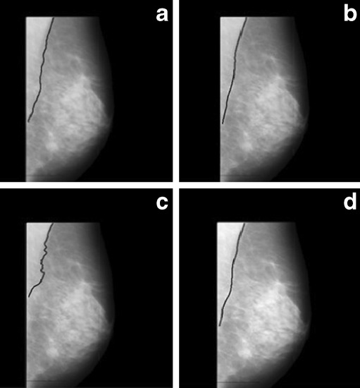
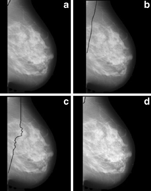
Images having pectoral muscle region with adjacent dense tissue are one of the most challenging images for pectoral muscle detection. Figure 10 shows one of such image with the segmented pectoral muscle region obtained by the proposed method, Ferrari’s method, and Kwok’s method.

Fig. 10.

Image mdb199 with pectoral muscle edge drawn a manually, b by proposed method, c by Ferrari’s method, and d by Kwok’s method

Pectoral muscle detection in dense breast is also a difficult job as the desired region and surrounding region have almost similar densities. Figure 11 demonstrates that the segmentation with the proposed method is better than the other two approaches. Segmentation failed for the other two methods.

Fig. 11.

Image mdb053 with pectoral muscle edge drawn a manually, b by proposed method, c by Ferrari’s method, and d by Kwok’s method. No segmented region is obtained by Ferrari’s and Kwok’s method

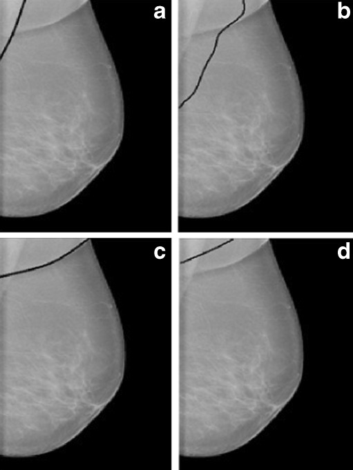
It is observed from the experiment that irrespective of the pectoral muscle segmentation techniques, CR images are the most difficult among all the three types of mammograms due to the similar intensity profile of the pectoral muscle region and the surrounding region. For these types of images, edge-based techniques like the proposed method and Ferrari’s method work better than threshold-based Kwok’s method as shown in Fig. 12.

Fig. 12.

CR image with pectoral muscle edge drawn a manually, b by proposed method, c by Ferrari’s method, and d by Kwok’s method

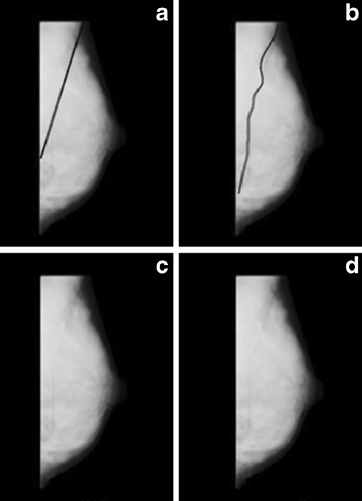
In general, for MLO view, the pectoral muscle should be seen to the level of the nipple [17]. So, muscle should not contain a very small region. But in few cases, due to improper positioning of the breast, exception occurs. For images with small pectoral muscle, Kwok’s method detect them accurately, whereas, the proposed method and Ferrari’s method sometime fail in detection (Fig. 13).

Fig. 13.

Image mdb031 with pectoral muscle edge drawn a manually, b by proposed method, c by Ferrari’s method, and d by Kwok’s method

As mentioned previously, CR images are the most challenging type among the mammograms irrespective of the pectoral muscle detection method used. One of such images is shown in Fig. 14 where all the methods have failed to detect pectoral muscle region. However, the number of such images is small (4 out of 40 CR images).

Fig. 14.

CR image with pectoral muscle edge drawn a manually, b by proposed method, c by Ferrari’s method, and d by Kwok’s method

Conclusion

This paper presents a new algorithm for automatic identification of pectoral muscle. The method first approximates the pectoral muscle boundary as a straight line using largest (pectoral) edge segment followed by smooth curve approximation using adaptive local search. Both of the steps are mainly based on sharp intensity variation at the pectoral muscle edge. Proposed algorithm is tested over three different types of mammogram images viz. scanned film (mini-MIAS), DR, and CR and compared with two well-known pectoral muscle detection algorithm proposed by Ferrari et al. [10] and Kwok et al. [11]. Results show proposed method outperforms the other two algorithms in terms of total mismatched pixel percentage, Housdorff distance, and MDCP. Experiment also confirms that among the three types of database, CR images are the most difficult irrespective of all the three methods. It is noted that the accuracy of the present pectoral muscle detection algorithms leave room for improvement.

References

- 1.Garcia M, Jemal A, Ward EM, Center MM, Hao Y, Siegel RL, et al. Global cancer facts and figures 2007. Atlanta: American Cancer Society; 2007. [Google Scholar]
- 2.Cancer facts and figures 2011. Atlanta: American Cancer Society; 2011. [Google Scholar]
- 3.Gupta R, Undrill PE. The use of texture analysis to delineate suspicious masses in mammography. Phys Med Biol. 1995;40:835–855. doi: 10.1088/0031-9155/40/5/009. [DOI] [PubMed] [Google Scholar]
- 4.Hatanaka Y, Hara T, Fujita H, Kasai S, Endo T, Iwase T. Development of an automated method for detecting mammographic masses with a partial loss of region. IEEE Trans Med Imaging. 2001;20:1209–1214. doi: 10.1109/42.974916. [DOI] [PubMed] [Google Scholar]
- 5.Karssemeijer N. Automated classification of parenchymal patterns in mammograms. Phys Med Biol. 1998;43(2):365–378. doi: 10.1088/0031-9155/43/2/011. [DOI] [PubMed] [Google Scholar]
- 6.Saha PK, Udupa JK, Conant EF, Chakraborty DP, Sullivan D. Breast tissue density quantification via digitized mammograms. IEEE Trans Med Imaging. 2001;20:792–803. doi: 10.1109/42.938247. [DOI] [PubMed] [Google Scholar]
- 7.Ferrari RJ, Rangayyan RM, Desautels JEL, Frere AF: Segmentation of mammograms: identification of the skin—air boundary, pectoral muscle, and fibro-glandular disc. In IWDM 2000. Proc. 5th Int Workshop Digital Mammography 573, 2001
- 8.Kinoshita SK, Azevedo Marques PM, Pereira RR, Jr, Rodrigues JA, Rangayyan RM. Radon-domain detection of the nipple and the pectoral muscle in mammograms. J Digit Imaging. 2007;21(1):37–49. doi: 10.1007/s10278-007-9035-6. [DOI] [PMC free article] [PubMed] [Google Scholar]
- 9.Yam M, Brady M, Highnam R, Behrenbruch C, English R, Kita Y. Three-dimensional reconstruction of microcalcification clusters from two mammographic views. IEEE Trans Med Imaging. 2001;20(6):479–489. doi: 10.1109/42.929614. [DOI] [PubMed] [Google Scholar]
- 10.Ferrari RJ, Rangayyan RM, Desautels JEL, Borges RA, Frere AF. Automatic identification of the pectoral muscle in mammograms. IEEE Trans Med Imaging. 2004;23(2):232–245. doi: 10.1109/TMI.2003.823062. [DOI] [PubMed] [Google Scholar]
- 11.Kwok SM, Chandrasekhar R, Attikiouzel Y, Rickard MT. Automatic pectoral muscle segmentation on mediolateral oblique view mammograms. IEEE Trans Med Imaging. 2004;23(9):1129–1140. doi: 10.1109/TMI.2004.830529. [DOI] [PubMed] [Google Scholar]
- 12.Bajger M, Ma F, Bottema MJ. Minimum spanning trees and active contours for identification of the pectoral muscle in screening mammograms. In: Digital Image Computing: Techniques and Applications conference. 47–53, 2005
- 13.Ma F, Bajger M, Slavotinek JP, Bottema MJ. Two graph theory based methods for identifying the pectoral muscle in mammograms. Pattern Recogn. 2007;40(9):2592–2602. doi: 10.1016/j.patcog.2006.12.011. [DOI] [Google Scholar]
- 14.Wang L, Zhu M, Deng L, Yuan X. Automatic pectoral muscle boundary detection in mammograms based on markov chain and active contour model. Journal of Zhejiang University-SCIENCE C. 2010;11(2):111–118. doi: 10.1631/jzus.C0910025. [DOI] [Google Scholar]
- 15.Cardenosa G. Clinical breast imaging: a patient focused teaching file. Philadelphia, PA: Williams & Wilkins; 2006. [Google Scholar]
- 16.Seth S, Mukhopadhyay S, Das P, Bhattacharya P. Shape based breast segmentation in mammograms. IETE Journal of Research, 2011 (in press)
- 17.Paredes ESD. Atlas of mammography. 3. Philadelphia: Williams & Wilkins; 2007. [Google Scholar]