Automated regional analysis of B-mode ultrasound images of skeletal muscle movement

Abstract

To understand the functional significance of skeletal muscle anatomy, a method of quantifying local shape changes in different tissue structures during dynamic tasks is required. Taking advantage of the good spatial and temporal resolution of B-mode ultrasound imaging, we describe a method of automatically segmenting images into fascicle and aponeurosis regions and tracking movement of features, independently, in localized portions of each tissue. Ultrasound images (25 Hz) of the medial gastrocnemius muscle were collected from eight participants during ankle joint rotation (2° and 20°), isometric contractions (1, 5, and 50 Nm), and deep knee bends. A Kanade-Lucas-Tomasi feature tracker was used to identify and track any distinctive and persistent features within the image sequences. A velocity field representation of local movement was then found and subdivided between fascicle and aponeurosis regions using segmentations from a multiresolution active shape model (ASM). Movement in each region was quantified by interpolating the effect of the fields on a set of probes. ASM segmentation results were compared with hand-labeled data, while aponeurosis and fascicle movement were compared with results from a previously documented cross-correlation approach. ASM provided good image segmentations (<1 mm average error), with fully automatic initialization possible in sequences from seven participants. Feature tracking provided similar length change results to the cross-correlation approach for small movements, while outperforming it in larger movements. The proposed method provides the potential to distinguish between active and passive changes in muscle shape and model strain distributions during different movements/conditions and quantify nonhomogeneous strain along aponeuroses.

skeletal muscles are often composed of architecturally and/or physiologically distinct regions or compartments (8, 10), and it has been shown that different regions of a muscle can be activated to complete different motor tasks (26), at different points of a stride (9) or pedal cycle (25), and to generate forces in different directions (23). Identifying regional variation in muscle activity does not, however, provide insight into local changes in muscle shape. Such measures are required to 1) fully understand the functional significance of muscle-tendon unit anatomy (fascicle length/orientation, aponeurosis properties/interaction with fascicle region, tendon compliance, etc.); 2) explore the relationship between muscle architecture and the distribution of physiological properties; and 3) explore the dynamic interaction between passive and active tissue components during different motor tasks.

B-mode ultrasound provides a noninvasive method of visualizing skeletal muscle in vivo during completion of a range of dynamic tasks. Manual assessment of images is time consuming and open to subjective operator error. In addition, such an approach does not take advantage of the good spatial resolution in these images (∼185 μm, with measures of movements as small as 5 μm possible; Ref. 13) and means that localized movements that occur in the muscle may not be detected or accurately quantified. Ultrasound images also have good temporal resolution, with recordings at 25 Hz typical and measures as high as 5,000 Hz possible (7). Restrictions on operator time will likely reduce the number of participants, trials, and frames, which can be practically assessed within/between experimental protocols. To make full use of the information present in the collected images a quantitative, mathematical assessment of their properties is required. Such a tool requires the development and application of automated/semiautomated and accurate image segmentation and tracking techniques. While such techniques are widely available in the literature (see Ref. 11) their specific adaptation and application to images of skeletal muscle are sparse and therefore limit the current application of B-mode ultrasound for assessment of musculoskeletal properties in both clinical and research environments.

Tracking skeletal muscle features in ultrasound images is challenging. The process must cope with features that undergo significant changes in appearance or disappear from the ultrasound plane. The few approaches currently in the literature commonly involve manual identification of a number of feature windows or templates in a single reference frame and then tackle an absolute (frame-reference frame) and/or relative (frame-frame) correspondence problem using a Lucas-Kanade tracker (15) or cross-correlation (13). Both of the documented approaches rely on feature persistence, but neither addresses the occurrence of feature loss, so the deformation of features must be tolerated as the template is updated in the relative correspondence step. In the absence of any measure of whether the feature remains distinctive and good for tracking, there is a risk that the template becomes bland, corresponding well with many areas of the image and increasing potential error in the tracking by drifting. Therefore, for small movements (e.g., posture), where features persist and maintain a close likeness to the template, point-based tracking methods can provide good measures of localized muscle movement with subpixel resolution (13). However, they are not able to provide accurate measures during larger movements where features deform or are lost from the image plane. One further example of a point based feature tracker using the Lucas-Kanade algorithm has been documented for tracking movement of the musculotendinous junction (11). Here a central pixel, within an 11 × 5 pixel window located over the landmark of interest, was defined in the first frame and velocity fields in the region-of-interest were used to update its position. The approach was only tested for tracking this well-defined region of the muscle, and further application to assess movement of different/multiple regions was not attempted.

An alternative to tracking movements of given features within the image is to quantify changes in intensity within defined regions (20). This has been used to define mean fascicle orientation using Radon transform (21) and to define shape and movement of fascicles or tendon using discrete wavelet transform (DWT) (17, 20, 21). In all cases, manual initialization and definition of the region(s) of interest are required. In addition, their ability to independently study movement of the different tissues within the muscle, i.e., fascicles and aponeurosis, has not been explored.

To facilitate investigation of the functional significance of muscle structure and regional changes that occur during larger activations, we wished to develop a method to quantify regional variation in muscle shape change. Such a method should be capable of quantifying regional variations in strain along structures such as aponeuroses, facilitate modeling of localized strain distributions during active and passive movements, and have the potential to distinguish between active and passive changes in muscle shape. To do this, we present a novel combination of techniques from the computer vision and graphics literature enabling 1) automatic segmentation of skeletal muscle into anatomically distinct regions using a multiresolution active shape model (ASM; Ref. 5); 2) tracking of features within each region for the time they persist on the ultrasound cross-section using a Lucas-Kanade feature tracker with translational consistency check (14, 24); 3) automatic replacement of lost features with distinctive new features suitable for tracking (22); and 4) estimation of movement in each region from the displacements of transient features using particle tracing.

METHODS

Ultrasound Image Collection

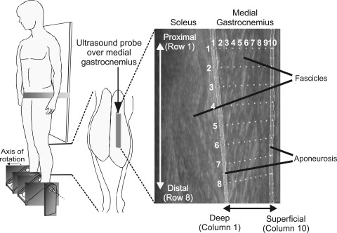
B-mode ultrasound images (Aloka ProSound SSD-5000, UST-5712 probe) were collected (25 Hz) from the medial gastrocnemius (MG) muscle of eight participants. Participants stood on a pair of instrumented footplates, which were used to either rotate the ankle joint through 2 or 20° range of motion or provide feedback for the participant to produce 1-, 5-, or 50-Nm isometric moments about the ankle joint (Fig. 1). In addition, participants completed a series of deep knee bends. During each task, ultrasound images were collected synchronously with angle and moment signals from the footplates using custom written MATLAB and SimuLink scripts running in a real-time environment (Real Time Windows Target toolbox). Images were collected over a 40-s period (1,100 images per subject). The work was approved by the Ethics Committee for the Faculty of Science and Engineering at Manchester Metropolitan University and complied with the principles laid down by the Declaration of Helsinki. All participants gave informed consent to the work.

Fig. 1.

Schematic representation of setup used to collect ultrasound images. Participant stood on two footplates, supported by a waistband wrapped around a fixed vertical board. Ultrasound probe (grey block) was placed over the midbelly region of the medial gastrocnemius (MG) muscle. Ultrasound images reveal the MG and soleus muscles, with superficial corresponding to the region closest to the skin and deep corresponding to the region of muscle closest to the tibia. Configuration of probes, automatically placed on the first image of a sequence, within the segmented regions of medial gastrocnemius is also shown (vertical lines and small points, see methods for full explanation). Initial configuration was a 10 × 8 grid (column and row numbers denoted in white). For comparison of tracked muscle movements using the cross-correlation approach (13), templates were manually placed along the deep and superficial aponeurosis in the most representative frame. Templates across the fascicle region were then positioned using interpolation, providing the same configuration shown.

Image Segmentation

For the description and evaluation of the image segmentation approach, images collected during the first 30 s (750 frames) of the knee bends trial were used. This condition was chosen as it produced larger variations in MG movement and shape changes than the other conditions and therefore facilitated training of a diverse shape model (see appendix a, ASM Parameters).

Learning a points distribution model.

Points distribution models (PDMs) can be used to capture shape variations undergone by biological structures in images. To create a PDM (4), training data were generated by manually labeling 75 frames (every 10th frame) of the knee bend image sequences collected from each participant. Labels consisted of 19 points, 30 pixels (∼3.3 mm) apart, placed along each of the four boundaries of the two aponeuroses. We therefore produced M = 600 training images, each containing the two-dimensional locations of the 76 hand-labeled landmarks and hence 152 degrees of freedom (D_y = 2 × 76 = 152). Annotation of M training images resulted in a set of 600 state vectors, Y = {y₁, . . . ,y_M}, where the m^th training shape is denoted by y_m.

A model of shape variation was then recovered by the application of principal component analysis to the resulting spatial distributions, reducing the dimensionality (D_y = 152) of the dataset. The mean shape ȳ and covariance matrix S were calculated from Y and singular value decomposition (SVD) was used to find the eigenvectors, ϕ_i and eigenvalues, χ_i of S. This allowed for an estimate of any data point, y_m, spanned by the training set using the relationship

$$y{\prime }_m=\overline{\mathbf{y}}+\Phi x_m,$$ 1

where Φ = [Φ₁,Φ₂ . . . ,Φ_Dx] contains the first D_x eigenvectors corresponding to the largest eigenvalues, and the latent variable x_m is given by

$$x_{\mathit{m}}={\left(x_{\mathit{m}}^1,...,x_{\mathit{m}}^{D_x}\right)}^{\text{T}}={\Phi }^{\text{T}}\left({\mathbf{y}}_m-\overline{\mathbf{y}}\right).$$ 2

With the use of this relationship, the training data Y are approximated by a set of latent variables X = {x₁, . . . ,x_M} where the dimensionality D_x < D_y is selected to preserve some minimum fraction of the variance in the original data set, here 98.5%. With the use of the approximation in Eq. 1, a shape can be fully specified using a single low-dimensional weighting vector x taken from the resulting latent shape space.

ASM training.

An ASM (3, 6) augments a PDM with Gaussian models of image intensity at each landmark to allow a probabilistic search for known shapes in new images. Following Cootes and Taylor (3), intensity models are learned by sampling a normalized intensity gradient along a straight line extending k pixels (here k = 2 equivalent to 0.22 mm, see appendix a for details) to either side of a given landmark and running perpendicular to the local PDM contour. Sampling is repeated across the set of all M training images to give a set of samples G = {g₁, . . . ,g_M} for each landmark. The samples for a given landmark are then modeled by a (2k + 1)-dimensional Gaussian distribution by estimating a mean vector ḡ and a diagonal covariance matrix S_g. In the multiresolution approach (5) texture models are also estimated at a number of lower image resolutions (see appendix a), three in the work presented here, to facilitate a coarse-to-fine search for solutions, as detailed below.

Fitting an ASM to new images.

During fitting, the task of the multiresolution ASM is to adjust the set of landmarks in the PDM to accurately describe shapes in a previously unseen, image. The fitting process (5) is initialized with the PDM's mean shape hypothesis ȳ. Each landmark is then permitted to move along a fixed, straight line extending n_s pixels to either side of its current location and running perpendicular to its connections to its neighbors. Landmarks are moved pixel-by-pixel along this line, and new intensity samples were drawn to determine their most likely location given the new image and the pretrained texture model. The likelihood of a new normalized sample g′ given a texture model g ∼ N(ḡ,S_g) can be quickly evaluated by calculating the Mahalanobis distance,

$$f\left(\mathit{g}\prime \right)={\left(\mathit{g}\prime -\overline{\mathit{g}}\right)}^{\text{T}}{\mathit{S}}_g^{-1}\left(\mathit{g\prime }-\overline{\mathit{g}}\right),$$ 3

which is proportional to the log of the probability that g′ was generated by the Gaussian distribution g ∼ N(ḡ,S_g). Once Eq. 3 has been minimized for every landmark, the new shape configuration is projected into the PDM's latent space (using Eq. 2) and the nearest plausible shape is found by shifting to within 3 SD of the latent variables X.

The comparison process is repeated 10 times at each image scale, moving from the lowest-resolution image to the original high-resolution image with a constant search range of n_s = 3 pixels (see appendix a for details). Because this search range is a constant, independent of the current image resolution, the result is an effective “coarse-to-fine” search able to make large initial landmark adjustments in the lower resolution images before smaller refinements in the subsequent higher-resolution images.

ASM extensions for skeletal muscle: ASM*.

The previous two sections describe the application of a standard multiresolution ASM from the computer vision literature. Here we detail a number of modifications, denoted by ASM*, that we have found to be valuable for processing images of skeletal muscle. First, as the shape change between consecutive video frames is small we appeal to a simple model of temporal consistency and initialize the ASM search of a frame with the shape solution from the previous frame, rather than the PDM's mean shape, ȳ. Second, as we have observed greater consistency in the size of aponeuroses across subjects than in the thickness of MG, we take steps to weaken interaponeurosis correlations in the PDM. This is done by reducing the off-diagonal elements of S that give the covariance between deep and superficial aponeuroses to 20% of their original values before the application of SVD (see Learning a points distribution model). Note that this step has no effect on intra-aponeurosis correlations. Finally, to avoid losing small shape variations seen in the superficial aponeurosis during PDM construction, we “whiten” this subportion of the state vectors in the training set Y. For a given shape y_m = (y_m¹, . . . ,y_m¹⁵²)^T the first 76 degree of freedom relate to the superficial aponeurosis y_m^s = (y_m¹, . . . ,y_m⁷⁶)^T and the second 76 to the deep aponeurosis y_m^d = (y_m⁷⁷, . . . ,y_m¹⁵²)^T. We calculate the respective mean aponeuroses ȳ^s and ȳ^d and equalize the respective standard deviations about each shape by scaling up the spatial distribution of {y_m^s}_{m = 1}^M about its mean to give σ^s = σ^d. This causes the equal retention of variations in both aponeuroses during PDM learning, shifting 98.5% of the variance across ∼10 eigenvectors.

Automatic initialization: ASM*_B.

The standard multiresolution ASM (5) fits independently to each test image, always commencing its search from the PDM's mean shape, ȳ. The alternative settings ASM* have the ability to give smoother segmentations, but require accurate initialization at the first frame. Initialization could be provided manually, but here we also explore the potential for automating this challenging initial segmentation. To do this we add two further image resolutions (1:8 and 1:16) to the ASM* training procedure, giving a total of five pyramid levels. This allows the ASM* to make larger landmark adjustments early on in the search, but fitting remains a local method that may still converge to an incorrect solution. To address this we avoid using the mean shape (ȳ) to initialize the search and instead start N separate searches, each commencing from the mean shape of one of the subjects in the training set. At the end of this new search procedure, we have N different shape solutions from which we select the one with the lowest greyscale Mahalanobis distances (Eq. 3) across all landmarks and all image resolutions. Although this search strategy, which we denote with ASM*_B, is more expensive, it is suitable for initialization, after which we can revert to using the ASM* settings for frame-to-frame tracking. To facilitate evaluation and cross comparison of the segmentation process we stipulated that initialization occur at frame one.

Evaluation of image segmentation.

Evaluation of image segmentation was completed in a leave-one out fashion, whereby the training data from the participant who was being assessed was excluded from the construction of the required shape and texture models. Each evaluation therefore represents fitting of an unknown subject using training images from the remaining subjects and replicates the situation where an initial training set has been established (here N = 7) and images from a new, previously unseen, participant are assessed with no prior labeling or manual input from the operator. The excluded subject's manually labeled frames provided a record of ground truth for quantitative evaluation. In each labeled frame, error was calculated as the absolute distance between the 76 predicted and hand-labeled landmarks. A total of 6,000 ultrasound images were segmented.

Tracking Features Within Images

For the description and evaluation of our approach to track features within the collected ultrasound images, all 1,100 recorded frames (40 s trial duration) from each experimental condition are presented. The shape model used for image segmentation was trained on images recorded during knee bending conducted in a leave-one out approach, as described in Evaluation of image segmentation.

Feature selection.

In the presented work, square feature templates of size 15 × 15 pixels (∼1.65 × 1.65 mm, approximately the size of smallest features in the images) were defined. This enabled ∼200 nonoverlapping feature templates to be identified in images of ∼450 × 450 pixels. Features were identified as suitable for tracking by consideration of the Hessian of an image I(x,y)

$$H=\left[\begin{array}{cc}\frac{{\partial }^{2}I}{\partial x^2}& \frac{{\partial }^{2}I}{\partial x\partial y}\\ \frac{{\partial }^{2}I}{\partial y\partial x}& \frac{{\partial }^{2}I}{\partial y^2}\end{array}\right]$$ 4

(22). The eigenvalues of this matrix, λ₁ and λ₂, give a measure of the local curvature in the pixel intensity surface. Two large values imply corners, which are particularly good for tracking. Both eigenvalues for a candidate feature window are therefore set to exceed a minimum threshold, min (λ₁,λ₂) > λ, here λ = 500 (see appendix a for details). This approach to feature detection means that if templates identified in the first frame do not persist in subsequent frames, they can be automatically replaced with new, good, features as soon as they appear.

Feature tracking.

Feature templates identified using Shi and Tomasi's (22) detection technique were tracked from frame to frame using Lucas-Kanade feature tracking (KLT). The goal of this algorithm is to align a feature template T(x, y) with a new image I(x, y) through a translational warp w(x, y; p) = [x + p₁, y + p₂]^T. This is achieved by minimizing some measure, f, of the difference between the two regions in a registration process,

$$p_{\text{reg}}={\arg }_{\text{p}}\min \mathit{\text{f}}(\mathit{\text{I}}(\mathit{w}(\mathit{x},\mathit{y};\mathit{p})),\mathit{T}(\mathit{x},\mathit{y}))$$ 5

Lucas-Kanade tracking uses a sum of squared differences to evaluate the difference measure f and Quasi-Newton descent to solve the optimization problem in Eq. 5 in an iterative gradient descent approach. Importantly, there are a number of simple criteria that can be used to declare a feature template lost. These include an inability to reach a minimum change in translation parameters within a set number of iterations, loss of intensity gradient within the template, features templates overlapping with the image borders, and large residues between the past and present template.

We use the symmetric KLT implementation of Birchfield (1) to select and to track ultrasound image features, using the default settings with a template smoothing factor of 0.01 (see appendix a for details) and incorporating the translational consistency check. The consistency check ensures that a mapping exists between the original template and the feature window recovered at the current frame. This extra criterion by which a feature may be declared lost guards against the gradual deformation of the original feature when working in a relative (frame-to-frame) correspondence framework.

Quantifying movement in fascicle and aponeurosis regions.

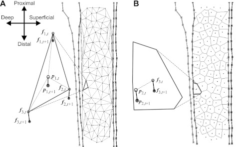
As the proposed KLT approach employs automatic feature detection, it differs from previous approaches (13, 15) because it does not rely on the persistence of specific features through all frames. We must therefore estimate tissue movement based on the collection of automatically defined KLT features that come and go throughout the sequence. To do this we define a set of measurement probes, placed across the image at the initialization frame based on the image segmentation results. Here, eight probes are placed along both the deep and superficial aponeurosis, and a further 64 were placed across the fascicle region (Fig. 1). This probe placement is achieved fully automatically, based on the ASM segmentation. The movement of each probe is determined by the movement of all persisting feature tracks on the ASM segment (e.g., deep/superficial aponeurosis or fascicle region) within which it lies. KLT features are divided between ASM segments (Fig. 1), and a set of displacement fields (one per segment) are estimated by finite differencing the locations of all templates that have persisted from the last frame. The result is a collection of irregular vector fields composed of a variable number of elements from which we must interpolate displacement values at the location of every probe (Fig. 2). We use triangle-based linear interpolation to update probes that lie within each feature set's convex hull and nearest neighbor interpolation for those that lie outside. This is achieved by calculating the Delaunay triangulation (Fig. 2A) and Voronoi diagram (Fig. 2B) for each feature set, respectively. Probes are free to move outside the image, with their position updated using nearest neighbor interpolation from a Voronoi diagram calculated from persisting features in all segments. This gives sensible movements where no ultrasound information is available and allows probes to move back into view during cyclic activity.

Fig. 2.

Interpolation of Lucas-Kanade feature tracking (KLT) feature displacement fields within the fascicle region of MG. Delaunay mesh (A) and Voroni cell (B) interpolation procedures for example probes p₁ and p₂ (inside and outside the convex hull, respectively), using locations of the persistent features set (f₁, f₂, f₃). Orientation of the muscle in both diagrams is shown in A.

In some of the 40 test sequences, blood vessels are visible in the fascicle region. Features in the vessels can score well in terms of their Hessian eigenvalues but, due to the pulsating blood flow, tend to be short lived and to drift across the vessel. They therefore do not capture movement of the muscle tissue. To identify and discount these features from the assessment of movement in the fascicle region, we estimate the mean μ_t, and SD σ_t, of all feature lifetimes in the fascicle region and exclude those templates that have persisted for less than (μ_t − σ_t) from the interpolations described above. In the majority of sequences, this criterion has little or no effect, but where the fascicle region is relatively still and blood vessels are visible they are prevented from disturbing probes (see also Supplementary Video SMV7_VesselExclusion_True; Supplemental Material for this article is available online at the J Appl Physiol website).

Evaluation of proposed feature tracking.

To enable comparison of the proposed tracking method with an existing technique applied in physiological experiments, we also assessed ultrasound images from all trials using spatial cross-correlation, following Loram et al. (13). For this method, a representative frame was selected from each trial and eight templates of size 15×24 pixels (∼1.65 × 2.64 mm) were manually placed along the two aponeuroses. In an extension to the published methods, intermediate rows of templates were placed between the aponeuroses using interpolation (Fig. 1), reflecting a manual implementation of the automatically placed measurement probes in the proposed approach. Each template was then tracked, using the two-pass approach detailed in Loram et al. (13), through all frames of the trial.

Calculation of reported measures.

Changes in muscle length relate to force output and change in joint angle (12) with a broadly linear relationship. To determine the quality of our tracking, we used Pearson product-moment correlation to quantify the relationships between muscle displacement and ankle joint angle (passive movements) or ankle moment (isometric contractions), respectively, measured from the footplate apparatus. The same calculations of displacement were applied to results from both feature tracking approaches.

All calculations are described relative to the anatomical orientation of the muscle during standing, as depicted in Fig. 1. Within each row the vertical distance between marker pairs in the outer two columns (columns 1 and 10 in Fig. 1) were calculated. This measure represents the relative longitudinal movement of the two aponeuroses and was termed aponeurosis displacement. In addition, the vertical distance between marker pairs in each row of the fascicle region (columns 3 and 8 in Fig. 1) were also calculated, quantifying relative longitudinal movement within that region and termed contractile tissue displacement. Aponeurosis and contractile tissue displacements were calculated relative to initial length. Thus eight measures of aponeurosis displacement and eight measures of contractile tissue displacement were calculated per image and correlated with the relevant footplate measure. To identify the mean performance across the image within each subject, the mean correlation was calculated for each displacement. Significant differences between results from the baseline and the proposed approach were identified within each condition using Wilcoxon signed rank test (P ≤ 0.05).

RESULTS

Assessment of Proposed Segmentation Approach

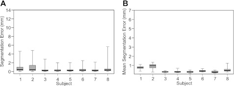
The search for segmentations was manually initialized at the first frame of each sequence. Figure 3A shows the absolute errors of all 76 points of the ASM* segmentations across all hand-labeled frames of the knee bend sequences (76 × 75 = 5,700 errors per box) of every participant. Across landmarks within each frame (i.e., average error within each frame), ASM* gives small errors across the remaining images (<0.5 mm across all landmarks in 6 participants and <1 mm in all subjects; Fig. 3B) and low variation in the magnitude of the error across participants. Results obtained using a standard multiresolution ASM without the modifications detailed in ASM extensions for skeletal muscle: ASM* are included for comparison in appendix b.

Fig. 3.

Box and whisker plots showing the error of the segmentation using the active shape model extensions for skeletal muscle (ASM*) in each participant. Error was the absolute distance between the manually and ASM* defined position of each landmark. A: errors calculated from each landmark within each analyzed image (total 76 landmarks × 75 frames = 5,700 points in each box). B: mean error from all landmarks within each image (total 75 frames = 75 points in each box), providing an indication of the overall quality of the image segmentation. In both plots, middle bar represents the median value, bottom and top of the box represent the 25th and 75th percentiles, respectively, and the whiskers represent the minimum and maximum values. See appendix b, for comparison of results with a standard ASM.

Assessment of Automatic Initialization

We tested the ability of ASM*_B settings to automatically initialize segmentation by comparing with manually defined segmentations across 75 images from each participant. The average absolute difference across the 76 landmarks between hand-labeled and ASM segmentations (segmentation errors) averaged across the 75 analyzed images are shown in Table 1. We also evaluated the performance of a five-layer ASM* as a baseline for comparison. Automatic initialization was possible for the majority of participants with both parameter settings (e.g., >73/75 correct initializations). Across all participants, the average initialization error was reduced by searching for a segmentation from a number of different initializations (ASM*_B) (Table 1). Poor initialization consistently occurred in S8, with ASM* and ASM*_B only providing accurate initialization in 28/75 and 34/75 cases, respectively. This relates to the poorly defined superficial boundary of the deep aponeurosis, combined with the presence of a nearby, dark blood vessel in collected images (see Fig. B2B in appendix b). This combination of factors meant that the blood vessel was repeatedly misidentified as a boundary of the deep aponeurosis (see Implications of Fully Automated Image Segmentation for further discussion).

Table 1.

Results of automatic initialization experiments using settings ASM* and ASM*_B

	Participant
	S1	S2	S3	S4	S5	S6	S7	S8
ASM* good initialization	73	75	75	73	75	75	66†	28†
ASM* average error, mm	0.71	0.37	0.29	0.35	0.29	0.34	0.68	1.92†
ASM*B good initialization	74	75	75	73	75	75	75	34†
ASM*B average error, mm	0.63	0.30	0.28	0.30	0.28	0.30	0.27	2.01†

Good initialization shows the total number of images (out of 75) that were fitted with <1 mm average error and average error (in mm) across all 75 frames is also reported. ASM, active shape model; ASM*, ASM extensions for skeletal muscle; ASM*_B, automatic initialization.

^†Cases where poor initialization was common.

Assessment of Proposed Feature Tracking Approach

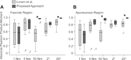
To facilitate comparison between tracking approaches we stipulated that initialization occur at frame one. This meant manually initializing the segmentation of all of subject 8 (S8) trials (N = 5), but each of the remaining subjects' sequences (N = 35) were all successfully initialized by ASM*_B. Compared with the cross-correlation approach, the proposed approach resulted in significantly higher correlation values for both aponeurosis and contractile tissue displacement during 20° ankle joint rotation and 50-Nm isometric contraction (P = 0.012, all cases; Fig. 4). No significant differences existed between approaches for the other conditions.

Fig. 4.

Box and whisker plots showing Pearson product-moment correlation for footplate signal (torque or ankle joint angle) and the proposed approach (dark boxes) or the cross-correlation approach (13) (lighter boxes) for the fascicle region (A; contractile tissue displacement) and the aponeuroses (B; aponeurosis displacement). Asterisks denote significant differences between approaches (P < 0.05). Middle bar represents the median value, bottom and top of the box represent the 25th and 75th percentiles, respectively, and the whiskers represent the minimum and maximum values (less outliers, which are shown as individual points and labeled with the appropriate participant number; N = 8).

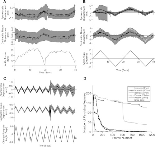
Representative traces of aponeurosis and contractile tissue displacement during three experimental conditions in one participant are shown in Fig. 5, A–C. The mean aponeurosis and contractile tissue displacements (calculated from the eight rows of the feature grid, see Fig. 1) of the proposed approach for the 50-Nm isometric contraction (Fig. 5A) and 20° ankle joint rotation (Fig. 5B) were very smooth, with low SDs, and highly correlated with the torque (aponeurosis displacement: r = −0.93, contractile tissue displacement: r = −0.96) and angle (aponeurosis displacement: r = 0.97, contractile tissue displacement: r = 0.97), respectively. In contrast, the mean displacements calculated from the cross-correlation approach (13) include some large and unphysiological changes in length (e.g., Fig. 5B, 0–10 s), with very high SD. The correlation values were also much lower (angle: aponeurosis displacement r = 0.54, contractile tissue displacement r = 0.76; torque: aponeurosis displacement r = −0.48, contractile tissue displacement r = −0.60).

Fig. 5.

Changes in aponeurosis length and contractile tissue displacement for a representative subject (S6) during 50-Nm isometric contraction (A), 20° ankle joint rotations (B), and 2° ankle joint rotations (C). Each displacement graph shows results from the proposed approach (mean: black, broken line; ±1 SD: light grey shaded area) and the cross-correlation approach (13) (mean: black, solid line; ±1 SD: dark grey shaded area). Mean and SD values were calculated from displacements of the 8 rows of regions of interest (see Fig. 1). Note how the mean displacement from the proposed approach and the cross-correlation approach are often in close agreement but that the variation in these data is much higher for the cross-correlation approach, especially for the larger movements. Recorded ankle torque and angle are shown at bottom (grey line). D: persistence of features present in frame 1 over subsequent image frames for each condition. Note the rapid drop in the number of persisting features for larger movements.

The persistence of features, present in the first frame, over the course of each sequence in Fig. 5 (and all other experimental sequences from the participant) are shown in Fig. 5D. During smaller movements (2° ankle joint rotation and 1-Nm isometric contraction) where the cross-correlation approach (13) performed well, features persist for a large proportion of the sequence. For 2° ankle joint rotation, the sudden drop in persisting features at approximately frame 660 (25 s) corresponds to a large jump in aponeurosis and contractile tissue displacement (and the SD across grid rows) calculated using the cross-correlation approach, while the proposed approach continues to produce smooth displacements (Fig. 5C). During larger movements (20° ankle joint rotation, 50-Nm isometric contraction), features present in the first frame rapidly disappear from the image in just a few frames. It is also important to note that for the larger movements the variation in displacements calculated across the eight rows were much higher for cross correlation and therefore only the mean displacement value is a robust measure (Fig. 5).

DISCUSSION

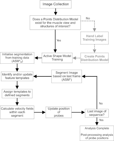
To date, very little work has applied computer vision techniques to track skeletal muscle features recorded using B-mode ultrasound. This has meant much work has been completed using manual digitization of images, which may not make full use of the spatial resolution in collected images. An overview of the workflow for the proposed approach is shown in Fig. 6, with two possible routes that may be required during implementation. Route one (grey, broken lines) illustrates the situation when images are collected from a muscle not previously studied. If a suitable PDM does not exist, it is necessary to hand label a proportion of the collected images before analysis. Here the PDM consisted of 75 frames from 1 trial in each of 7 subjects (therefore not including the subject studied). In our experience, this initial input required ∼9 h investment (7 subjects × 75 frames × ∼60 s). We labeled a large number of images to construct robust ASMs but also to provide sufficient testing data for thorough quantitative evaluation (see Assessment of Proposed Segmentation Approach and Assessment of Automatic Initialization). We have also obtained similar segmentation accuracy for the same range of movements with much lower sampling rates, e.g., labeling every 100^th training image, requiring <1 h initial time investment.

Fig. 6.

Schematic representation of the steps required for image segmentation and feature tracking.

Once the PDM is established, the second route in the workflow (black, solid lines) may occur, whereby a new participant enters the laboratory or new data are collected. In this instance, images can be automatically segmented and feature tracking occurs in a fully automated process. We found that fully automated, first frame initialization and processing were possible in 7/8 participants (35/40 trials) and, with a suitable experimental protocol, automatic initialization can be quickly achieved even in more challenging subjects (see Implications of Fully Automated Image Segmentation for further discussion).

Implications of Fully Automated Image Segmentation

Image segmentation means that only those features centered in the same region of interest are used in the interpolation of its probes, providing a means by which interactions between anatomically distinct tissues can be quantified. To minimize the overlap of individual templates with other regions we used small template windows roughly equal to the aponeurosis and fascicle widths in the image. Although small overlaps may still occur, the translational consistency check ensures that no such template will persist through any relative movement between the two regions. To our knowledge, this work represents the first attempt to independently and simultaneously estimate movement in the fascicle region and the aponeuroses (Figs. 5–6). In Loram et al. (13), each template occupies ∼10–15% of the image width and those on the deep aponeurosis contain portions of aponeurosis, gastrocnemius, and soleus tissue. Radon transform and DWT (21) have only been used to provide information on features within the fascicle region, while tracking of the fascicle region is not attempted by Magnusson et al. (15) and the question of overlap from the superficial aponeurosis is not addressed (e.g., the template size is not quoted). Our approach therefore lays a foundation for independently quantifying movement in different tissue components, an important step in understanding the dynamics between active and passive tissues during different motor tasks, and also provides a means through which strain along specific structures (e.g., aponeuroses) may be calculated (also see Potential Investigations of In Vivo Muscle Behavior).

In B-mode images, the appearance of tissue boundaries depends not only on a step change in acoustic impedance but also on their distance from, and angle relative to, the transducer. The muscle structures in the lower leg are well suited to investigation with intensity derivatives as the boundaries of interest run parallel to the skin and perpendicular to the transducer. As the ASM provides a texture model, based on intensity derivatives, it is well suited to defining tissue boundaries and active appearance models, which developed from ASM principles, have been applied to ultrasound images before (2, 18, 19). We believe, however, this is their first application to skeletal muscle. Alternative methods of image segmentation are available in the literature. For example, the application of active contours is a popular method of recovering tissue boundaries from B-mode image intensity derivatives (16). This approach however, does not allow for modeling long-range intracontour correlations. Indeed no intercontour correlations can be modeled as active contours do not parameterize the variation in contour shapes, relying only on edge-strength, size, and smoothness heuristics to find boundaries. The consistent meaning of ASM landmarks across sequences and subjects allows for long range correlations to be captured as easily as short range correlations during training. When applied to new images, the resulting ASM boundaries have consistent physiological meanings, which in our approach have permitted the automatic division of features between anatomical regions and the automatic placement of probes at initialization.

In this study, we have used manual initialization at the first frame to ensure that every available frame was processed and facilitate cross comparisons; this is not, however, a requirement for others interested in adopting the approach. As initialization only needs to be successfully performed once (with ASM* used for subsequent frame-to-frame tracking), in situations where poor initialization occurs at frame one, we would recommend introducing a short extra initialization procedure where ASM*_B is repeatedly reapplied to subsequent images from the sequence. Taking the example of knee bends for the challenging subject S8 and applying the findings of Assessment of Automatic Initialization, there is still a probability of 34/75 that ASM*_B will be successful on any given image from this participant. The probability of getting one or more successful initializations from a group of five randomly selected knee bend images is therefore, 1 – (41/75)⁵ = 0.95, or 95%. The reapplication of ASM*_B can be controlled (e.g., through a simple button press) until a suitable initialization is achieved in a process likely to take only a few seconds.

Implications of Automated Feature Tracking

In the physiological literature, the tracking algorithm of Loram et al. (13) is the only method shown to track small muscle movements with high resolution (5 μm). We therefore consider it represents a gold standard when used in situations when features in the image do not deform or become lost, i.e., smaller movements. Comparing the results of this benchmark and the proposed approach reveals equivalent performance for small movements (2° ankle joint rotation; 1- and 5-Nm isometric contraction; Fig. 4). The proposed approach therefore matches benchmark standards for these movements. Large variations in the results for 1 and 5 Nm are apparent in both approaches (Fig. 4), which may be the result of nonlinearity in the relationship between torque and displacement. In some instances, however, it seems as though subjects were able to complete these low force tasks with no/minimal movement, and probably little activation, of MG (see Supplementary Videos SMV4_1Nm and SMV5_5Nm).

Performance of the standard was worst when participants performed the largest voluntary contraction (50 Nm; Figs. 4–5) probably reflecting the reduction in feature persistence that occurs in larger movements (Fig. 5D). In contrast, performance of the proposed approach dramatically improves with larger movements (20° ankle joint rotation; 50-Nm isometric contraction; Figs. 4–5). Relying on collections of transient features, rather than individual persistent features, therefore means we have been able to retain the benefits of point-based trackers (e.g., Refs. 13, 15), specifically quantifying movement in different regions of the muscle (Fig. 7), while also being able to accurately assess larger movements.

Fig. 7.

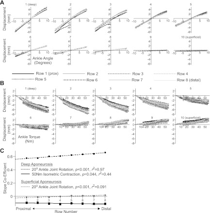
Vertical displacement of all probes during 20° ankle joint rotations (A) and 50-Nm isometric contractions (B) from participant S2. All values have been normalized to position at the first frame. Each graph displays displacement of all probes within the defined column (1–10, see Fig. 1), with each row (1–8, see Fig. 1) defined by line style. In both conditions, the largest differences in the pattern of displacement occur from deep to superficial regions (comparing graphs 1–10 in A and B). Note: 1) how the pattern of displacement within each graph is more dispersed during isometric contractions, a consistent feature across all participants and potential indicator of active vs. passive changes in muscle shape (see Distinguishing Between Active and Passive Muscle Movements); and 2) differences in displacement direction between deep and superficial regions during active contraction but not passive ankle joint rotation. C: slope coefficients describing the best fit line fitted to plots of vertical displacement vs. angle (circles, 20° condition) or torque (squares, 50-Nm condition) of each of the 8 probes in the deep (black, column 1) and superficial (grey, column 10) aponeurosis (i.e., each line in graphs 1 and 10 in A and B). Data were taken from S7. Data points are shown where regression analysis revealed a significant relationship across row position: deep aponeurosis during both active and passive conditions; the superficial aponeurosis during passive ankle joint rotations, with details provided in the graphic.

One methodological consideration of the proposed approach is the potential for tracks to gradually drift, as the sequential nature of the processing means that position errors could accumulate over time. The implementation documented does not require the probes within each segment to return to a particular configuration and plotting the vertical displacement of probes relative to joint angle indicates that drift was not apparent in the current data set (Fig. 7A, note displacements consistently pass through the zero point). For experimental conditions when a cyclical event occurs (i.e., a pedal cycle, stride, etc.), such a requirement could potentially be incorporated based on assessment of features (re)appearing at a consistent point within the pedal/stride cycle.

Further work is also required to determine the performance of the approach for assessment of a larger range of movements as well as segmentation and tracking of different muscle groups. We found good performance for assessment of deep knee bending movements (see Supplemental Video SMV8_KneeBendMvt) but have yet to test the approach on more challenging locomotor conditions where identifying a gold standard for quantitative evaluation is more difficult. If muscle shapes encountered during any new experimental protocols are similar to those in the current PDM, it is likely that the accuracy of image segmentation will be maintained. Larger movements, and particularly rapid movements, are, however, likely to further reduce feature persistence and lead to more rapid feature tracking error accumulation. As such, our tracking approach may not be as robust and we would expect the ability to quantify regional movement to be reduced. In addition, the robustness of the approach when applied to lower resolution/quality images from other ultrasound machines could be explored (see also appendix a, Feature Selection).

Potential Investigations of In Vivo Muscle Behavior

In the following sections, we provide insights into some physiological investigations which are now possible using our approach. These are initial, exploratory findings only, and further, specific, experiments are required to fully investigate how generally applicable they may be.

Distinguishing between active and passive muscle movements.

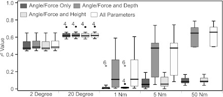
Within the current data set, the pattern of probe movements differed between passive and active conditions. Figure 7B, shows that, for a 50-Nm isometric contraction, probes in the superficial and deep muscle regions respectively moved proximally and distally relative to the ultrasound probe (also see Supplementary Video SMV1_50Nm). In contrast, during 20° ankle joint rotation all probes moved in the same direction with only the amount of movement differing across deep-superficial regions (also note the much smaller divergence across rows; Fig. 7A). Regression analysis revealed that for ankle joint rotation, angle alone was the best predictor of vertical probe displacement (Fig. 8). The inclusion of probe location, with depth defined by column number and proximal-distal location defined by row number (see Fig. 1), did not significantly improve prediction ability. In contrast, for isometric contractions the inclusion of probe depth significantly improved prediction of displacement, especially for the 50-Nm condition (Fig. 8). Regional information of probe displacement could therefore be a useful discriminator between active and passive muscle movements, and further work should explore the potential for ultrasound imaging to provide a means of identifying activation under different conditions. Such a tool would be particularly valuable for the assessment of deep muscle structures, which are readily visualized with ultrasound, but activation can currently only be assessed using invasive fine-wire electromyography procedures.

Fig. 8.

Box and whisker plots representing results of multiple regression analysis, predicting displacement of all 80 probes. For each condition four analyses were conducted, with dependent variables defined as angle/force only (dark grey boxes), angle/force and deep-superficial depth (col. number, Fig. 1; midgrey boxes), angle/force and proximal-distal location (row number, Fig. 1; light grey boxes), and all parameters (angle/force, depth and proximal-distal location; white boxes). Analysis for all subjects and each of the 5 experimental conditions are shown. Middle bar represents the median value, and bottom and top of the box represent the 25th and 75th percentiles, respectively, and the whiskers the minimum and maximum values (less outliers, which are shown as individual points and labeled with the appropriate participant number); N = 8.

Quantifying aponeurosis strain.

The segmentation of images into anatomically distinct tissue structures provides, in some instances, the opportunity to quantify strain along the aponeurosis. Care is required, as in collected images aponeurosis tissue is quite bland and not feature rich. Predictions of probe movements in images where the aponeurosis is for example very thin could rely on tracking of very few features and may therefore not robustly represent regional movement along the segment. In the current data set, the aponeuroses of S7 both consistently contained ∼12 features. For this participant, we plotted the vertical displacement of all eight probes in the deep and superficial aponeurosis, as in Fig. 7, A and B, graphs 1 and 10, for 20° ankle joint rotations and 50-Nm isometric contraction. We calculated the line of best fit for each of the eight lines in both aponeuroses. The slope coefficient of each line is shown in Fig. 7C as a function of proximal-distal location (row number, Fig. 1). For 20° ankle joint rotations there was a significant linear relationship across proximal-distal location in both deep (P < 0.001; r² = 0.97) and superficial (P < 0.001; r² = 0.91) aponeuroses. This revealed greater displacement in the distal region of the deep aponeurosis and different directional movement in the superficial aponeurosis. During 50-Nm isometric contractions, the relationship altered and while proximal-distal location was still a significant factor in the deep aponeurosis (P = 0.04; r² = 0.44) the relationship was weak and it was not significant in the superficial aponeurosis (Fig. 7C). This suggests that patterns of tissue displacement along the aponeurosis differ between active isometric contractions and passive ankle joint rotations and is potentially influenced by the location and distribution of activated fibers.

Similar analyses could also be conducted on any of the probes within the grid, quantifying regional differences in muscle movement (Fig. 7, A and B), a calculation not previously possible as the average movement across probes was required for a robust result (Fig. 5). Movement across the probe grid will, in part, be influenced by the relative proportion of active and passive tissue components, determined by the size and distribution of activated motor units and the level, nature, and distribution of connective tissue components. Such properties will change with aging and progression of neurodegenerative diseases and are likely to impact force transmission from the activated fibers to the joint; potential for sensory feedback from different muscle regions and the interaction between synergistic muscles. Our approach facilitates investigation of these relationships and a fuller understanding of their impact on coordinated force production. Future work should investigate whether the tracking approach could be adapted to enable automated quantification of fascicle length, shape, and/or orientation. In its present form, the approach offers a robust method of quantifying skeletal muscle shape changes and movement in fascicle and aponeurosis tissues during a wider range of movements than previously possible. It should also be noted that being fully automated and sequential (unlike: 13) also makes real time implementation a possibility, which would facilitate experimental work where biofeedback is desirable.

APPENDIX A: ASM AND KLT PARAMETER SETTINGS

ASM Parameters

Training a points distribution model.

In the current work, PDM training data were generated by manually labeling every 10th frame of the image sequence collected from each participant as they performed deep knee bends. This activity was chosen as it produced varied movement and shape changes within MG and therefore could provide a diverse range of shapes with which to train the PDM. Researchers interested in compiling their own training set should consider the tasks/activities participants are to complete, and the training sequences should come from an activity which produces a spectrum of muscle shape changes which will encompass those likely to be seen during the task(s) of interest.

Intensity gradient sampling and image scales.

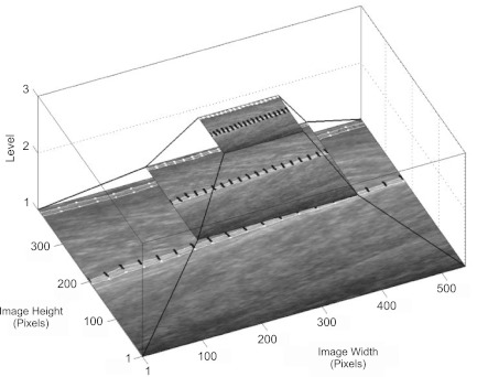
Figure A1 illustrates the pyramid of image scales used in the multiresolution approach texture models (see ASM training). Intensity models are learned by sampling a normalized intensity gradient along a straight line running perpendicular to the local PDM contour. The use of normalized gradients should provide some insensitivity to the different imaging settings of different ultrasound machines, e.g., image contrast/brightness. The smallest search range that reliably encapsulates the intensity step change between the appearance of aponeurosis (light) and muscle fascicles (dark) in the images is defined as k. We sampled k = 2 pixels (∼0.22 mm) either side of each landmark, and we recommend this distance value be maintained. As the intensity step changes are not immediate, using k = 1 risks failing to span the full intensity change surrounding a given landmark. Increasing k is unlikely to provide any benefit from as there is no further consistent intensity information further away the landmarks (perpendicular to the boundary), except when 1) one side of the intensity profile stretches right across an aponeurosis and spans the intensity step change at the far boundary; and 2) profiles on the superficial aponeurosis reach beyond the image edge.

As k is a constant, the real physical distance that is spanned by two pixels doubles every time one moves up a search level in the image pyramid. At the top (lowest resolution image) of the five-layer pyramid used by ASM*_B during initialization (see Automatic initialzation: ASM*_B), k = 2 spans its maximum value to either side of every landmark (∼3.5 mm). This comfortably stretches right across aponeuroses and stretches from the superficial aponeurosis to beyond the image edge. The latter boundary is a particularly useful cue, implicitly capturing the depth of the superficial aponeurosis. To make use of this feature, we recommend drawing samples from a buffer of zero values when outside the image.

Search range (n_s).

The number of pixels either side of a point that is searched is defined by n_s (see Fitting an ASM to New Images). This value is also a constant across pyramid levels, meaning that quite large movements may occur at coarse levels (Fig. A1, pyramid top), with more refined movements occurring as the image resolution grows (Fig. A1, pyramid bottom). We found n_s pixels was the smallest search range that reliably gave good segmentation results. The value must be a large enough physical distance that ASM* can cope with sudden shape changes (1.32 mm at the top of the pyramid) and ASM*_B can successfully initialize from the nearest subject mean (5.27 mm), but any larger and we risk wasting computation time.

Fig. A1.

Pyramid of image scales. Each level is half the size of the level below, with resolutions of 1:1, 1:2, and 1:4, across levels 1–3, respectively. Intensity models are learned by sampling a normalized intensity gradient along a straight line (black lines) extending k = 2 pixels either side of a given landmark (white dots) and running perpendicular to the local PDM contour (white lines). Sampled region is shown for the top boundary for the deep aponeurosis only.

Weakening interaponeurosis correlation.

We propose weakening the interaponeurosis correlation in the PDM by reducing the off-diagonal elements of S that give the covariance between deep and superficial aponeuroses before the application of SVD (see Learning a Points Distribution Model and Automatic Initialzation: ASM*_B). This is because we have observed much greater consistency in the size of the aponeuroses across subjects than in the thickness of MG. For example, the deep aponeurosis of S8 is much deeper than in any of the other participants whose images make up the PDM training set. The PDM cannot therefore accurately segment images from S8 as the required relationship between aponeuroses is not part of its repertoire. It is, however, important not to completely disregard/uncouple the inter-aponeurosis correlations within the PDM, as they are meaningful and potentially provide useful shape information. We therefore weakened the interaponeurosis correlations until we arrived at the first value (20%) that permitted S8 to be successfully segmented. This value retained as much interaponeurosis correlation information as possible, while also permitting a wider range of shape variations in the PDM. Other researchers may consider adjusting the 20% value if they use N > 7 training subjects or see greater similarity across subjects.

KLT Feature Selection and Tracking Parameters

Feature selection.

When selecting features to track, the corners of larger structures (corner features) are ideal as they permit the horizontal and vertical components of subsequent motion to be resolved. Corner features have λ₁ ≥ λ₂ > 0 (see Ref. 22) and so can be detected with a simple lower threshold λ = min(λ₁,λ₂) (see Feature selection). In the presented work, good coverage of distinctive features across the image was provided by λ = 500 with a template size of 15 × 15 pixels. Typically, 200 nonoverlapping features on a 450 × 450 pixel image (∼49.50 × 49.50 mm) were found. Raising the minimum threshold too high risks excluding good tracking features, but reducing it to a lower nonzero value may be useful, e.g., to ensure sufficient feature numbers when processing lower quality images. However, reducing λ too close to zero means that nondistinctive features (which are prone to drift) may be included, e.g., edges where λ₁ > λ₂ = 0 and homogeneous regions where λ₁ = λ₂ = 0. Inclusion of instantaneous ultrasound speckle patterns is also a possibility, but as these have zero persistence in time they will not contribute to probe movement.

Template smoothing factor.

A symmetric KLT implementation (1) was run with the default settings, a template smoothing factor of 0.01 and the translational consistency check. Smoothing the image attempts to eradicate local minima in the cost surface (sum of squared differences between intensities), which could distract the search procedure from finding the globally best match between template and image. A smoothing factor ∼0.1 is suitable for images of the real world (also see Ref. 1). Ultrasound images are, however, very different to real world images, especially in the muscle fascicle region where regular, repeating patterns occur. Accidentally matching feature templates with nearby physical structures that have a similar appearance is therefore a potential problem. Reducing the smoothing factor requires an even closer match between template and image, as small differences in the intensity patterns are not smoothed away. This can increase the risk of recovering local minima (and missing the global minimum); however, the strict translational consistency check guards against this possibility, as unless the image patch found by the Newton-Raphson matching process is a translational warp of the original feature template, tracking will be deemed to have failed and the template will be discarded.

APPENDIX B: STANDARD ASM: SEGMENTATION COMPARISONS WITH ASM*

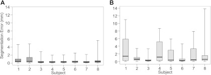
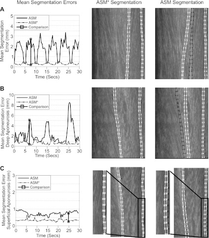
Figure B1, A and B, shows the mean segmentation error across all landmarks and all frames for each participant. ASM* provides a consistent fit for all participants (Fig. B1A) and likely reflects the use of a temporal model by ASM*, where we assume only small movements between consecutive frames and the segmentation from the previous frame is used to initialize the search at the current frame. In contrast, the standard ASM searches from the mean shape at each frame and occasionally fails, producing large error magnitudes (Fig. B1B). In five participants, landmark errors greater than 6 mm are recorded, with errors greater than 10 mm occurring in two participants (S1 and S8). Figure B2A shows the mean segmentation errors of ASM and ASM* for a single subject over time. While ASM* segmentations closely match the manually defined location of both superficial and deep aponeurosis throughout the sequence, there are large portions of the knee bend cycle where the standard ASM is unable to identify the location of the deep aponeurosis.

Fig. B1.

Box and whisker plots showing the error of the segmentation using ASM* (A) and ASM (B) in each participant. Error was the absolute distance between the manually and ASM*/ASM defined position of each landmark. Plots show the error calculated from each landmark within each analyzed image (total 76 landmarks × 75 frames = 5,700 points in each box). Middle bar represents the median value, bottom and top of the box represent the 25th and 75th percentiles, respectively, and the whiskers represent the minimum and maximum values.

Figure B2B shows mean segmentation errors for images from participant S8, whose deep aponeurosis is particularly low compared with all other participants (e.g., compare Fig. B2, A and B, middle). ASM* reduces the covariance between the two aponeuroses during training, permitting them to vary with greater relative independence, and is able to recover good segmentations across the sequence (Fig. B2B). In contrast, the standard ASM is more rigidly constrained by the PDM training data and cannot generate novel shapes to segment the particularly low deep aponeurosis at 7, 15, and 25 s, giving mean errors of >4 mm per landmark in the deep aponeurosis (Fig. B2B).

Fig. B2.

Comparison of segmentation defined by ASM and ASM* illustrating how ASM* implementation outperforms the standard ASM settings. A: participant S3. B: participant S8; C: participant S2. Left: mean segmentation error calculated as the mean error of all 76 (A) and 38 landmarks (B and C) in each tested image from both ASM (black, solid line) and ASM* (grey, broken line). Vertical line highlights a time when segmentation using ASM* provides a more accurate recovery of the aponeurosis (middle) compared with segmentation using ASM (right). At middle and right, hand-labeled contours are shown in black, with the respective segmentation shown in white.

Figure B2C shows the quality of the superficial aponeurosis segmentation for S2. ASM* uses whitening to improve the retention of variations in the superficial aponeurosis by the PDM. This produces accurate segmentations in this region of the image, with mean errors consistently <0.5 mm per landmark in the superficial aponeurosis (Fig. B2C). In contrast, the standard ASM produces poorer segmentations in the distal region of the aponeurosis (Fig. B2C), with mean errors between 0.5 and 1 mm per landmark.

REFERENCES

- 1.Birchfield S.Derivation of Kanadi-Lucas-Tomasi Tracking Equation. (Online). http://www.ces.clemson.edu/∼stb/klt/
- 2. Bosch JG, Mitchell SC, Lelieveldt BPF, Nijland F, Kamp O, Sonka M, Reiber JHC. Automatic segmentation of echocardiographic sequences by active appearance motion models. IEEE Trans Med Imaging 21: 1374–1383, 2002 [DOI] [PubMed] [Google Scholar]
- 3. Cootes TF, Taylor CJ. Active shape model search using local grey-level models: a quantitative evaluation. In: BMVC1993. Surrey, UK: British Machine Vision Conference, 1993, p. 639–648 [Google Scholar]
- 4. Cootes TF, Taylor CJ, Cooper D, Graham J. Training models of shape from sets of examples. In: BMVC1992. Leeds, UK: British Machine Vision Conference, 1992, p. 9–18 [Google Scholar]
- 5. Cootes TF, Taylor CJ, Lanitis A. Active shape models: evaluation of a mulit-resolution method for improving image search. In: BMVC1994. York, UK: British Machine Vision Conference, 1994, p. 327–336 [Google Scholar]
- 6. Cootes TF, Taylor CJ, Lanitis A, Cooper D, Graham J. Building and using flexible models incorporating grey-level information. In: ICCV1993. Berlin, Germany: International Conference on Computer Vision, 1993, p. 242–246 [Google Scholar]
- 7. Deffieux T, Gennisson Jl Tanter M, Fink M. Assessment of the mechanical properties of the musculoskeletal system using 2-D and 3-D very high frame rate ultrasound. IEEE Trans Ultrason Ferroelectr Freq Control 55: 2177–2190, 2008 [DOI] [PubMed] [Google Scholar]
- 8. English A, Wolf SL, Segal RL. Compartmentalization of muscles and their motor nuclei: the partitioning hypothesis. Phys Ther 73: 857–867, 1993 [DOI] [PubMed] [Google Scholar]
- 9. Higham TE, Biewener AA, Wakeling JM. Functional diversification within and between muscle synergists during locomotion. Biol Lett 4: 41–44, 2008 [DOI] [PMC free article] [PubMed] [Google Scholar]
- 10. Kernell D. Muscle regionalization. Can J Appl Physiol 23: 1–22, 1998 [DOI] [PubMed] [Google Scholar]
- 11. Lee SS, Lewis GS, Piazza SJ. An algorithm for automated analysis of ultrasound images to measure tendon excursion in vivo. J Appl Biomech 24: 75–82, 2008 [DOI] [PubMed] [Google Scholar]
- 12. Loram ID, Maganaris CN, Lakie M. The passive, human calf muscles in relation to standing: the short range stiffness lies in the contractile component. J Physiol 584: 677–692, 2007 [DOI] [PMC free article] [PubMed] [Google Scholar]
- 13. Loram ID, Maganaris CN, Lakie M. Use of ultrasound to make noninvasive in vivo measurement of continuous changes in human muscle contractile length. J Appl Physiol 100: 1311–1323, 2006 [DOI] [PubMed] [Google Scholar]
- 14. Lucas BD, Kanade T. An iterative image registration technique with an application to stereo vision. In: International Joint Conferences on Artificial Intelligence, edited by Hayes PJ. Vancouver, British Columbia: 1981, p. 674–679 [Google Scholar]
- 15. Magnusson SP, Hansen P, Aagaard P, Brond J, Dyhre-Poulsen P, Bojsen-Moller J, Kjaer M. Differential strain patterns of the human gastrocnemius aponeurosis and free tendon, in vivo. Acta Physiol Scand 177: 185–195, 2003 [DOI] [PubMed] [Google Scholar]
- 16. Mikic I, Krucinski S, Thomas JD. Segmentation and tracking in echocardiographic sequences: active contours guided by optical flow estimates. IEEE Trans Med Imaging 17: 274–284, 1998 [DOI] [PubMed] [Google Scholar]
- 17. Namburete AIL, Rana M, Wakeling JM. Computational methods for quantifying in vivo muscle fascicle curvature from ultrasound images. J Biomech 44: 2538–2543, 2011 [DOI] [PubMed] [Google Scholar]
- 18. Noble JA. Ultrasound image segmentation and tissue characterization. J Eng Med 224: 307–316, 2009 [DOI] [PubMed] [Google Scholar]
- 19. Noble JA, Boukerroui D. Ultrasound image segmentation: a survey. IEEE Trans Med Imaging 25: 987–1010, 2006 [DOI] [PubMed] [Google Scholar]
- 20. Peolsson M, Lofstedt T, Vogt S, Stenlund H, Arndt A, Trygg J. Modelling human musculoskeletal functional movements using ultrasound imaging. BMC Medical Imaging 10: 9, 2010 [DOI] [PMC free article] [PubMed] [Google Scholar]
- 21. Rana M, Hamarneh G, Wakeling JM. Automated tracking of muscle fascicle orientation in B-mode ultrasound images. J Biomech 42: 2068–2073, 2009 [DOI] [PubMed] [Google Scholar]
- 22. Shi J, Tomasi C. Good features to track. In: Computer Vision and Pattern Recognition. Seattle, WA: 1994, p. 593–600 [Google Scholar]
- 23. Staudenmann D, Kingma I, Daffertshofer A, Stegeman DF, van Dieën JH. Heterogeneity of muscle activation in relation to force direction: A multi-channel surface electromyography study on the triceps surae muscle. J Electromyogr Kinesiol 19: 882–895, 2009 [DOI] [PubMed] [Google Scholar]
- 24. Tomasi C, Kanade T. Shape and motion from image streams: a factorisation method: Part 3 Detection and tracking point features. Pittsburgh, PA: Carnegie Mellon, School Computer Science, 1991 [Google Scholar]
- 25. Wakeling JM. The recruitment of different compartments within a muscle depends on the mechanics of the movement. Biol Lett 5: 30–34, 2009 [DOI] [PMC free article] [PubMed] [Google Scholar]
- 26. Wolf SL, Segal RL, English A. Task-oriented EMG activity recorded from partitions in human lateral gastrocnemius muscle. J Electromyogr Kinesiol 3: 87–94, 1992 [DOI] [PubMed] [Google Scholar]
Associated Data
This section collects any data citations, data availability statements, or supplementary materials included in this article.