

Abstract
To quantify the contribution of sensory information to multisegmental frontal plane balance control in humans, we developed a feedback control model to account for experimental data. Subjects stood with feet close together on a surface that rotated according to a pseudorandom waveform at three different amplitudes. Experimental frequency-response functions and impulse-response functions were measured to characterize lower body (LB) and upper body (UB) motion evoked during surface rotations while subjects stood with eyes open or closed. The model assumed that corrective torques in LB and UB segments were generated with no time delay from intrinsic musculoskeletal mechanisms and with time delay from sensory feedback mechanisms. It was found that subjects' LB control was primarily based on sensory feedback. Changes in the LB control mechanisms across stimulus amplitude were consistent with the hypothesis that sensory reweighting contributed to amplitude-dependent changes in balance responses whereby subjects decreased reliance on proprioceptive cues that oriented the LB toward the surface and increased reliance on vestibular/visual cues that oriented the LB upright toward earth vertical as stimulus amplitude increased in both eyes open and closed conditions. Sensory reweighting in the LB control system also accounted for most of the amplitude-dependent changes observed in UB responses. In contrast to the LB system, sensory reweighting was not a dominant mechanism of UB control, and UB control was more influenced by intrinsic musculoskeletal mechanisms. The proposed model refines our understanding of sensorimotor integration during balance control by including multisegmental motion and explaining how intersegmental interactions influence frontal plane balance responses.
Keywords: feedback control model, sensory reweighting
the dynamic characteristics of frontal plane balance control in humans were recently explored in our laboratory (Goodworth and Peterka 2010b). Subjects adopted several stance widths while continuous medial-lateral surface tilt perturbations were used to evoke lower body (LB) and upper body (UB) sway responses. Response dynamics varied systematically with stance width and stimulus amplitude. However, the control mechanisms contributing to the experimentally observed dynamics could not be unambiguously determined from the experimental data alone because more than one mechanism could potentially account for many of the results. For example, the observed reduction in responsiveness to the surface stimulus with increasing stimulus amplitude might be due to changes in passive stiffness of the body arising from co-contraction. Alternatively, the reduction might be due to changes in a neurally mediated feedback control strategy. In the current study, a multisegment parametric model was developed to distinguish between conflicting interpretations of previously obtained experimental data.
In the current study, we specifically focused on developing a model to aid our understanding of the experimental data obtained in a narrow stance condition (ankles separated by a few centimeters). In this condition, both LB and UB sway responses were dependent on the amplitude of the surface-tilt stimulus in that subjects became relatively less influenced by the surface-tilt stimulus as the stimulus amplitude increased (Goodworth and Peterka 2010b). This finding was similar to results from other frontal plane studies where subjects adopted a narrow stance (Cenciarini and Peterka 2006; Oie et al. 2002). In these previous studies, stimulus amplitude-dependent changes were attributed to a sensory reweighting mechanism whereby, with increasing stimulus amplitude, subjects decreased their reliance on orientation information derived from sensory systems that encode body orientation relative to the stimulus and increased their reliance on orientation information derived from sensory systems that encode body orientation relative to earth vertical. These interpretations were based on center-of-mass (CoM) motion. However, because CoM measures are determined by the orientation of individual body segments, a more complete understanding of sensory reweighting could be found if control mechanisms underlying multisegment control were known. A multisegment model that accounted for the detailed dynamic characteristics of stimulus-evoked motions of both the LB and UB could 1) determine whether sensory re-weighting does account for the observed amplitude-dependent changes in LB and UB, 2) determine whether changes in stance control mechanisms attributable to sensory reweighting occur in both LB and UB segments, 3) provide a detailed explanation about what control properties actually change when behavior attributable to sensory reweighting occurs, 4) determine whether mechanisms other than sensory reweighting (such as amplitude-dependent changes in the contribution of passive characteristics of muscle-tendon systems) contributed to the reduced responsiveness to external stimuli observed in our experimental findings, and 5) characterize changes in balance control attributable to access to accurate visual orientation cues.
Most existing multisegment balance control models have been developed to describe sway in the sagittal plane (Alexandrov et al. 2005; Barin 1989; Koozekanani et al. 1980; Kuo 1995, 2005; Park 2002; Park et al. 2004; van der Kooij et al. 1999). In these models, body segments are connected as an open-chain mechanical system with the bottom segment connected to the floor. Several important mechanisms of control have been identified and included in these sagittal plane models. For example, there is evidence that sensory feedback from segments across the entire body contributes to torque generation at each joint (Alexandrov et al. 2005; Barin 1989, Kuo 1995, 2005; Park 2002; Park et al. 2004) and that gain factors relating segment kinematics to torque generation change with stimulus amplitude and biomechanical constraints (Kuo 1995; Park 2002; Park et al. 2004).
For sway in the frontal plane, however, a different type of model is required. In the frontal plane, the LB forms a closed-chain mechanical system, and consequently, the equations governing LB motion depend on stance width. Previous studies have used models that account for the stance-width dependence of LB mechanics on frontal plane balance control (Bingham et al. 2011, Scrivens et al. 2008). However, these studies did not consider the influence of independent UB motion and the interactions between LB and UB control. Furthermore, there is evidence that pelvis orientation, which is a function of stance width, surface tilt, and LB sway, is an important kinematic variable influencing UB control (Goodworth and Peterka 2009, 2010a). It would therefore be beneficial to consider pelvis orientation in a model of frontal plane balance control. To our knowledge, there have been no published models of frontal plane sway that include these features.
Therefore, in the present study, a multisegment frontal plane model was developed that accounts for properties of the LB mechanical system and includes pelvis orientation. We applied this model to interpret our previous experimental results in a narrow stance condition, but the portion of the model describing the mechanics of frontal plane sway is defined so that it applies to a range of stance widths. Stability is achieved by generating corrective torques to control LB and UB motion via two mechanisms. Passive mechanisms, based on the intrinsic mechanical stiffness and damping properties in muscles, tendons, joints, and ligaments, generate torques with no time delay. Active mechanisms generate torques based on time-delayed muscle activation related to segment motion derived from sensory systems. By representing both passive and active mechanisms, the model is able to determine the relative importance of these mechanisms in regulating frontal plane balance. The model of frontal plane balance control is used to distinguish between competing interpretations of experimental results and therefore contributes to our understanding of frontal plane balance control.
METHODS
Experiment Description
Experimental data used in the current study were previously described (Goodworth and Peterka 2010b) and were obtained from the seven subjects who exhibited similar control strategies across all test conditions. All subjects gave their informed consent before being tested with the use of a protocol approved by the Institutional Review Board at Oregon Health & Science University. Below we briefly describe the test conditions and analysis that characterized postural dynamics.
Body sway was evoked in the frontal plane in freestanding subjects through continuous rotations of the surface on which subjects stood. Tests were performed with eyes open (EO) and eyes closed (EC) at four stance widths. Only data from the narrow stance condition (5-cm distance between medial malleoli and the inner margins of the feet aligned parallel to one another) were used in the current study. During EO tests, subjects viewed a stationary, complex checkerboard pattern lining a half-cylinder-shaped screen (70-cm radius) (Peterka 2002). Surface rotation was controlled by a servomotor, and the rotation axis was horizontal and perpendicular to the subject's frontal plane at ankle height centered between the subject's feet. The surface rotational stimulus, based on a pseudorandom ternary sequence (PRTS) (Davies 1970), was a pseudorandom velocity waveform with a 43.72-s cycle duration. The power spectrum of stimulus velocity had approximately equal amplitude spectral components ranging from 0.023 to about 16.7 Hz, which allowed characterization of the balance control system across a wide bandwidth, giving greater insight into the system dynamics compared with using a single stimulus frequency. The stimulus waveform was scaled to provide peak-to-peak position amplitudes of 1°, 2°, or 4°. Seven cycles of the PRTS waveform were presented in the lowest amplitude test, and six cycles were presented in the higher amplitude tests because responses to higher amplitude tests were large enough that low variance estimates of mean responses could be made with less averaging across individual stimulus cycles.
Average body dimensions of the seven subjects were as follows: mass, 68 kg; height, 172 cm; L4/L5 spinal joint above surface, 106 cm: greater trochanter above surface, 89.5 cm; hip joint center above surface, 91.2 cm; and distance between hip joint centers, 17.5 cm. The L4/L5 joint level was estimated as the iliac crest height (Skotte 2001). The UB segment mass and moment of inertia were calculated with respect to the L4/L5 joint. The distance between hip joint centers was estimated using a regression equation relating hip joint distance to inter-ASIS (anterior superior iliac spine) distance, and hip joint center height above the surface was estimated using a regression equation relating ASIS height to inter-ASIS distance (Seidel et al. 1995). Body segment mass and moment of inertia were estimated via anthropomorphic measures (Erdmann 1997; Winter 2005).
Experimental results that characterized LB and UB dynamics and that were used for comparison with model results were frequency-response functions (FRFs) and impulse-response functions (IRFs). An FRF is a nonparametric representation of the relation of a response signal to a stimulus signal through the decomposition of these stimulus-response signals into frequency components (Bendat and Piersol 2000). Each FRF was expressed as a set of gain and phase values that vary with frequency. Each gain value indicates the ratio of the amplitude of response variables (LB or UB sway) to the surface-stimulus amplitude at a particular stimulus frequency, and each phase value (expressed in degrees) indicates the relative timing of the LB or UB sway with respect to the surface stimulus. Estimates of IRFs were attainable because the PRTS velocity waveform approximated white noise (Davies 1970). IRFs were calculated by appropriately scaling the circular cross-correlation between the PRTS velocity waveform and the LB and UB sway velocity waveforms of each subject. This IRF calculation is described in detail in Goodworth and Peterka (2009). The IRF of a linear system is the time domain equivalent of the frequency-domain FRF (Westwick and Kearney 2003). Although the IRF and FRF representations of the system dynamics are equivalent, a time delay is easier to recognize in an IRF than a FRF, where its effects are distributed. Thus IRFs are particularly useful in distinguishing between control mechanisms that generate torque in relation to body sway without time delay (i.e., from intrinsic mechanical properties of muscles/tendons) and with time delay (i.e., from muscle activation via sensory feedback mechanisms).
Model Description
Frontal plane body mechanics were modeled as a two-segment, inverted-pendulum structure (i.e., LB and UB segments) with an additional representation of how pelvis orientation changes as a function of surface tilt and LB tilt (Fig. 1, A and B). Representation of the LB as a single segment is possible because the LB, consisting of two legs and a pelvis, is a closed-chain mechanical system with only one degree of freedom. The Appendix provides details of the two-segment model, including linearized equations of motion, linearized calculation of pelvis tilt angle, and the accuracy of the simplified system.
Fig. 1.
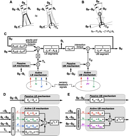
Block diagram of proposed lower body (LB) and upper body (UB) control system showing the simplified inverted pendulum representation of LB mechanics (A), the inverted pendulum representation of UB mechanics and pelvis orientation (B), a block diagram representing the equations of motion of the LB and UB segments (see Eqs. A1 and A2; the biomechanical factor R that scales LB torque is defined in Eq. A3) and LB and UB torques from passive and active control mechanisms (C), the input signals and control parameters that define the passive and active feedback mechanisms of the LB control system (D), and the input signals and control parameters that define the passive and active feedback mechanisms of the UB control system (E). Physical segment kinematic variables in the block diagram are represented by thick solid lines, sensory signals encoding segment kinematics or torques are represented by lowercase letters with dashed lines, and joint torques are represented by thin solid lines. The LB and UB control systems are closed loop, although lines representing feedback from sensory signals encoding segment angle, joint angles, and LB torque are omitted to enhance readability of the block diagram. The variable s is the Laplace variable. LB and UB control are not independent of each other because of interaction torques and because sensory-derived inputs to LB and UB control mechanisms are influenced by motions of both body segments and by the surface rotation. See text and Tables 1–3 for definition of sensory signals, time delays, torque feedback, and other parameters.
Stability and control of the two-segment model is provided by generation of LB and UB torques. UB torque (TU) is the summation of all torques generated from UB muscle activation (active UB mechanism) and intrinsic mechanical properties of the UB musculoskeletal system (passive UB mechanism) applied about a joint between the pelvis and UB. LB torque (TL) is the summation of all torques generated from LB muscle activation (active LB mechanism) and intrinsic mechanical properties of the LB musculoskeletal system (passive LB mechanism) applied about a single equivalent LB ankle joint. The two-segment mechanical model coefficients are scaled so that TL applied about this equivalent LB ankle joint produces the same motion as if TL were distributed equally among all four LB joints (i.e., ¼ of TL applied to each of the 2 ankle joints and 2 hip joints). The Appendix discusses the implications of assuming that TL is distributed equally among the two ankle joints and two hip joints in a closed-chain representation of the LB.
To quantify the control mechanisms contributing to stability, we assumed the two-segment mechanical model, represented as a block diagram in Fig. 1C, to be stabilized via corrective torques generated from a combination of active (i.e., muscle activation based on sensory signals encoding kinematics or kinetics of body motion) and passive (i.e., forces arising from intrinsic biomechanical properties of muscle/tendon systems) feedback control mechanisms. We investigated a large number of potential control schemes and tested each one by comparing model-predicted FRFs and IRFs with the experimental FRFs and IRFs. Each control scheme represents a quantitative hypothesis of how balance control mechanisms in the LB and UB function to stabilize the body. In the following paragraphs, we present a detailed description of the logic we used to identify a parsimonious control scheme that was able to account for the experimental results. In the discussion, we also address four other informative alternative control schemes.
Active control mechanisms were assumed to arise from feedback of sensory-derived internal estimates of body motion and orientation. The rationale for this assumption comes from psychophysical experiments where subjects were shown to be able to perceive multisensory and multisegmental aspects of body motion, such as trunk motion relative to the head (presumed proprioceptive origin) and head motion in space (presumed vestibular origin or combined proprioceptive-vestibular origin, depending on experimental conditions, when vision is absent), and were able to combine these signals to obtain estimates of segmental motions for which there were no direct peripheral sensors (e.g., trunk motion in space) (Mergner et al. 1991, 1993, 1997). Because subjects were able to perceive these segmental body motions, we assumed that this sensory-derived motion information was also available for feedback control of balance (Mergner and Rosemeier 1998; Mergner 2010). We also assumed that these sensory signals do not reflect the often nonlinear properties of primary sensory afferents, but represent signals processed by the central nervous system to more accurately encode multisegment body motion and orientation. There is neurophysiological evidence that the central nervous system has access to processed peripheral sensory signals that encode limb motion and orientation (Bosco and Poppele 1993; Bosco et al. 2000; Casabona et al. 2004) and that central mechanisms exist that combine peripheral vestibular semicircular canal and otolith signals to derive a representation of head orientation with respect to gravity (Angelaki et al. 1999, Merfeld and Zupan 2003).
The model input stimulus is the surface tilt angle (θS), and model output responses are UB tilt (θU) and LB tilt (θL) with respect to vertical. LB and UB control are not independent of each other because of interaction torques and because sensory-derived inputs to LB and UB control mechanisms are influenced by motions of both body segments and by the surface rotation. A detailed representation of the proposed LB and UB control mechanisms is provided in Fig. 1, D and E. To facilitate readability of these block diagrams, feedback lines have been omitted; however, LB and UB control mechanisms are based on feedback control, as described below.
The LB control generates TL based on passive and active mechanisms (Fig. 1D). The passive LB mechanism generates torque with no time delay in proportion to θS − θL (proportionality factor defined by the stiffness parameter KLi) and in proportion to the derivative of θS − θL (proportionality factor defined by the damping parameter BLi). This mechanism represents the intrinsic stiffness and damping from muscles, tendons, joints, and ligaments in the LB musculoskeletal system that tend to orient the LB perpendicular to the surface. The active LB mechanism generates torque from muscle contractions evoked in relation to signals from sensory systems that encode body motion and muscle torque. A time delay (τL) is present in the active mechanism due to neural transmission, central processing, and muscle activation delays. The active LB mechanism includes stiffness and damping parameters that determine the corrective torque generated in relation to sensory signals encoding various kinematic motion variables (i.e., angular positions and velocities of body motion). Table 1 defines the various sensory signals assumed to participate in LB and UB control. The LB stiffness parameters are symbolized by KL with the subscript extended to define the particular sensory signal with which it is associated (e.g., KLsl is associated with a proprioceptive signal encoding θS − θL). Similarly, the LB damping parameters are symbolized by BL with the subscript extended to define the particular sensory signal with which it is associated. The active LB mechanism includes an additional component of torque that is generated in relation to a sensory signal, tl, that encodes TL and is configured as a positive feedback control loop (Peterka 2003). This sensory torque signal, assumed to be low-pass filtered [first-order low-pass filter Laplace equation: GLt/(τLts +1)], provides additional feedback control that tends to move the LB toward an earth-vertical orientation. The sensory signal tl could be derived from Golgi-tendon organs or load sensors in the legs and feet.
Table 1.
Definition of sensory signals
| Sensory Signal | Definition | Sensory Origin |
|---|---|---|
| l | Encodes θL | Vestibular (EC) or vision/vestibular (EO) combined with intersegmental proprioception |
| lu | Encodes θL − θU | Proprioception |
| sl | Encodes θS − θL | Proprioception |
| u | Encodes θU | Vestibular (EC) or vision/vestibular (EO) combined with intersegmental proprioception |
| pu | Encodes θP − θU | Proprioception |
| tl | Encodes TL | Somatosensation (Golgi tendon organs, load receptors) |
Sensory signals are assumed to accurately encode physical variables. These sensory signals represent the output of central nervous system processing of information conveyed by primary sensory afferents (Angelaki et al. 1999; Casabona et al. 2004; Mergner et al. 1991, 1997). EC, eyes closed; EO, eyes open. Proprioception refers to sensory systems encoding of joint angles (body kinematics). Somatosensation refers to sensory systems encoding forces/torques (body kinetics). θL, lower body (LB) orientation; θU, upper body (UB) orientation; θS, support surface tilt angle; θP, pelvis orientation; TL, LB torque.
The UB control generates TU based on passive and active mechanisms (Fig. 1E). The passive UB mechanism generates torque with no time delay in proportion to θP − θU (stiffness parameter KUi) and in proportion to the derivative of θP − θU (damping parameter BUi) and tends to orient the UB perpendicular to the pelvis. The active UB mechanism generates torque based on a time-delayed (τU) summation of sensory feedback signals (defined in Table 1) multiplied by stiffness and damping factors. We did not find it necessary to include a torque feedback component for UB control.
Because the values of model control parameters determine the magnitude of corrective torque generated per unit of LB or UB sway, the relative contribution of passive vs. active control mechanisms to balance control were evaluated by comparing values of model parameters representing the contributions of passive and active control mechanisms. Also, changes in parameter values across test conditions were used to test the hypothesis that sensory reweighting accounted for the experimental FRF and IRF changes observed across test conditions. In previous studies, sensory reweighting has been defined as a subject shifting toward reliance on one source of sensory information while simultaneously shifting away from reliance on another source of sensory information (Allison et al. 2006; Ernst and Banks 2002, Peterka 2002). Therefore, in the current study, model parameters were used to determine whether the observed amplitude-dependent changes in body sway dynamics were due to sensory reweighting (indicated by a monotonic increase in at least one component of the active control mechanism accompanied by a monotonic decrease in at least one other active control component as stimulus amplitude increased) or, alternatively, were due to an increase in overall stiffness (indicated by an increase in one or more components of active control with increasing stimulus amplitude but not accompanied by a corresponding decrease in another component).
Estimation of Model Parameters
Model parameters associated with the mechanical model (ALU, JLU, ALS, JLS, JUL, JU, AU, JL, and AL; see Appendix) were determined for each subject based on anthropomorphic measurements. Remaining model parameters in Fig. 1 were associated with passive and active control mechanisms contributing to stabilization of the inherently unstable mechanical system. These control parameters were estimated from each subject's data by using a constrained nonlinear optimization routine, “fmincon” (Matlab Optimization Toolbox; The MathWorks, Natick, MA), to minimize a cost function equal to the sum of the mean squared errors from LB and UB FRFs of the normalized difference between model-predicted FRFs and experimental FRFs (Peterka 2002) at frequencies between 0.023 and 5.9 Hz. Fits to experimental FRFs (as opposed to IRFs) were used because we sought to characterize the system over a wide range of frequencies, and fitting to FRFs enabled us to equally weight the importance of all frequencies. After model parameters were obtained from fits to experimental FRFs, the model was used to generate model-predicted IRFs. Comparisons of experimental and model IRFs aided in verifying the FRF fit results, and comparisons were particularly useful in assessing the validity of model time-delay parameters. Stability was assessed for each subject's set of model parameters by predicting the 25-s time course of body sway evoked by a sudden surface tilt of 1° with a peak velocity of ∼35°/s using Matlab Simulink (The MathWorks). Model parameters were also estimated by applying the optimization procedure described above to fit the mean FRF data.
Selection of Model Parameters and Constraints
To describe the control mechanisms, we sought to increase confidence on parameter estimates by using the least number of parameters that account for the FRF and IRF data (Pintelon and Schoukens 2001). That is, we did not assume that all of the stiffness and damping parameters shown in Fig. 1, D and E, were necessary to include in the model. Several sensory feedback signals shown in Fig. 1 are analogous to signals shown in previous studies to be critical for balance control, whereas other feedback signals are less well understood and/or may be less critical. Therefore, we first assumed a basic model configuration that included feedback signals previously shown to be most critical for balance control, and then other, less well understood feedback signals were systematically added to determine which of these signals were necessary to explain the experimental data.
What we refer to as the “basic model” included the passive LB mechanism, active LB feedback of sensory signals encoding θL and θS − θL, LB torque feedback, the passive UB mechanism, and an active UB feedback of a sensory signal encoding θU. The rationale for including these particular sensory feedback mechanisms in the LB control system is that previous studies have shown that reliance on sensory signals that encode body-in-space and body-relative-to-surface are critical for control of body CoM (Cenciarini 2006; Maurer et al. 2006; Peterka 2002). Because we previously showed that LB FRFs are very similar to CoM FRFs (Goodworth and Peterka 2010b), we reasoned that LB feedback control needed to include sensory signals encoding θL and θS − θL in basic model structure. The inclusion in the UB control system of feedback from a sensory signal encoding θU was based on a previous study that demonstrated the importance of this control signal for spinal stability (Goodworth and Peterka 2009, 2010a). It was also recognized in previous studies that sensory signals encoding θP − θU and θL − θU (Goodworth and Peterka 2009, 2010a) might also contribute to UB control. However, with feet close together, the pelvis tilts in the same direction as the lower body, thus resulting in some redundancy between sensory signals encoding θP − θU and θL − θU. Thus we did not initially include these sensory signals in our basic model. Similarly, it was also unknown to what extent the intersegmental proprioceptive signals were critical to the LB control system, so sensory signals encoding θL − θU were not initially included in the basic model.
The decision to add additional sensory feedback parameters to the basic model was based on results from numerous model fits to the mean FRF data from the 2° stimulus amplitude trials in both EO and EC conditions. Model fits were performed that added one or more sensory feedback control parameters to the basic model. Judgments about the quality of the various model fits were based on their mean squared error.
Figure 2 shows the effect of including additional parameters on the quality of the model fit to the experimental FRF data. The inclusion of intersegmental damping, BLlu, in the LB control system made a very large improvement in the accuracy of the model. Additional improvement was made when intersegmental damping, BUlu, in the UB control system was included, particularly in the EO condition. Further improvement in both EC and EO conditions was achieved when the UB stiffness factor KUpu was included. Inclusion of additional parameters did not noticeably improve the model accuracy. Therefore, in both EO and EC, a parsimonious model was defined for use in the remainder of this study that included the basic model parameters (KLi, BLi, KLl, BLl, KLsl, BLsl, GLt, τLt, KUi, BUi, KUu, and BUu), intersegmental damping in LB control (BLlu), intersegmental damping in UB control (BUlu), and stiffness on the sensory signal encoding UB sway relative to the pelvis (KUpu) in the UB control system. Based on the analysis shown in Fig. 2, the parameters KLlu, KUlu, and BUpu did not contribute to improving fits to the LB and UB FRFs, and they were set to zero.
Fig. 2.
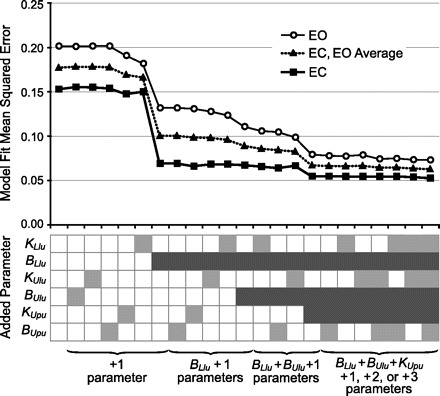
Identification of model active feedback control parameters that improved model fits (i.e., reduced mean squared error) to the experimental frequency-response function (FRF) data from 2° stimulus amplitude trials in both eyes closed (EC) and eyes open (EO) conditions. Mean squared error (top) is shown as model parameters, and combinations of parameters were added to the basic model (see text for definition of the basic model). Light and dark gray boxes (bottom) indicate which parameters were added to the basic model; dark gray boxes indicate parameters that produced noticeable reductions in the mean squared error and thus were retained in the final model configuration.
Most control parameters were allowed to vary across stimulus amplitude and between EO and EC, whereas a limited number of other parameters were fixed across stimulus amplitude. Time delays (τL and τU) and passive biomechanics (KLi, BLi, KUi, and BUi) were fixed across stimulus amplitude, since experimental IRFs showed no evidence for amplitude-dependent changes in the early time courses of the IRFs (i.e., <τL in the LB IRFs and <τU in the UB IRFs). Finally, the torque feedback time constant (τLt) was fixed across stimulus amplitude, because experimental FRF data showed no evidence for an amplitude-dependent influence of the torque feedback mechanism, which affects gain and phase data below about 0.1 Hz (see Fig. 6A).
Fig. 6.
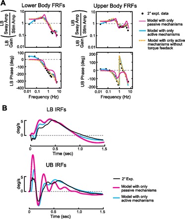
Predictions of alternative LB and UB control schemes. Predicted LB and UB FRFs (A) and impulse-response functions (IRFs; B) are shown for 2° amplitude tests based on model fits that included only active (blue lines) or only passive (red lines) control mechanisms. Results in A also show model-predicted FRFs when the LB torque feedback was eliminated (GLt = 0).
Model-Predicted FRFs and IRFs
Model-predicted FRFs were obtained by first calculating the Laplace domain expressions of θU(s)/θS(s) and θL(s)/θS(s), where s is the Laplace variable. These model-predicted FRFs included the mathematical expressions for both the mechanical system (defined by Eqs. A1–A3 in the Appendix) and the hypothesized feedback control mechanisms shown in Fig. 1. These expressions were obtained as a function of all model parameters by using the Matlab Symbolic Math Toolbox (The MathWorks). Model-predicted LB and UB FRFs were then obtained by substituting s = j2πf, where j is and f is frequency.
Model-predicted IRFs were calculated from simulated LB and UB sway using Matlab Simulink. Simulated LB and UB sway was evoked from surface rotations identical to the rotations measured from the surface during the experiments, and the simulated LB and UB responses were analyzed to calculate simulated IRFs in a manner identical to the method used to calculate experimental IRFs (Goodworth and Peterka 2009).
Statistics
Repeated-measures ANOVA was used to test for statistically significant effects of stimulus amplitude and EO vs. EC on model parameters. P < 0.05 was considered statistically significant.
RESULTS
Description of Model-Predicted FRFs and IRFs
Model-predicted FRFs were able to account for the detailed features of experimental LB and UB FRFs and IRFs in both EC (Fig. 3, A and C) and EO conditions (Fig. 4, A and C). For example, the model accounted for peaks in LB FRF gains at about 0.3 and 4 Hz, LB and UB phase leads below 0.15 Hz, local peak in LB phase at about 2.5 Hz, UB gain notch at about 1 Hz, and LB and UB gain reductions with increasing stimulus amplitude below 1 Hz. Model-predicted IRFs in both EC and EO conditions (Figs. 3C and 4C) were also very similar to experimental IRFs. For example, LB IRFs showed a brief initial negative peak at ∼0.05 s and then a first local maximum at ∼0.2 s, a second maximum at ∼0.5 s, a minimum at ∼1.5 s, and eventual decay to zero by 4 s (not shown in Figs. 3C and 4C). UB IRFs showed a large initial positive peak at ∼0.05 s, a negative peak at ∼0.2 s, a positive rise up to a local maximum at ∼0.7 s, and then an eventual decay to zero by 3 s (not shown in Figs. 3C and 4C). Stimulus amplitude-dependent changes were most noticeable after about ∼0.2 s in both LB and UB model-predicted IRFs consistent with experimental IRFs.
Fig. 3.
Model results for EC conditions. A: model-predicted (lines) and experimental (points) LB and UB FRFs for model fits where most parameters were allowed to vary across all stimulus amplitudes (unconstrained parameters, left) or where some parameters were constant across stimulus amplitude (constrained parameters, right). Model-predicted FRFs were from fits to mean FRF data. B: model parameters from unconstrained (left) and constrained fits (right). Open and filled symbols connected by lines are mean parameter values from model fits to individual subject FRF data; tinted error bars show SE. Points indicated by a cross (×) are parameter values obtained from model fits to the mean FRF data. C: experimental (expt.) LB and UB IRFs (left) and model-predicted IRFs (middle and right) based on model parameters from fits to mean FRF data.
Fig. 4.
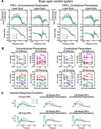
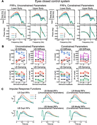
Model results for EO conditions. A: model-predicted (lines) and experimental (points) LB and UB FRFs for model fits where most parameters were unconstrained (left) or constrained (right). Model-predicted FRFs were from fits to mean FRF data. B: model parameters from unconstrained (left) and constrained fits (right). Open and filled symbols connected by lines are mean parameter values from model fits to individual subject FRF data; tinted error bars show SE. Points indicated by a cross (×) are parameter values obtained from model fits to the mean FRF data. C: experimental LB and UB IRFs (left) and model-predicted IRFs (middle and right) based on model parameters from fits to mean FRF data.
Model Control Parameters
EC parameters.
Parameter values related to intrinsic and sensory feedback mechanisms for balance control are shown in Fig. 3B for fits to mean FRFs (FRFs averaged across subjects) and fits to individual subject FRFs. Table 2 lists time delay and LB torque feedback parameters. Parameters estimated from fits to the mean FRFs were usually within 1 SE of mean parameters calculated from fits to individual subject FRFs.
Table 2.
Time delays and torque feedback parameters
| Fit to Individual FRFs |
Fit to Mean FRFs |
|||
|---|---|---|---|---|
| Parameter | Unconstrained | Constrained | Unconstrained | Constrained |
| EC τL, ms | 114 ± 3.6 | 115 ± 1.9 | 117 | 117 |
| EC τU, ms | 72.9 ± 6.5 | 71.1 ± 6.4 | 84.4 | 84.2 |
| EO τL, ms | 118 ± 4.5 | 117 ± 4.1 | 118 | 118 |
| EO τU, ms | 74.2 ± 9.3 | 67.1 ± 7.6 | 73.0 | 57.6 |
| EC τLt, s | 19.8 ± 5.3 | 17.6 ± 3.5 | 13.2 | 13.4 |
| EO τLt, s | 22.3 ± 5.7 | 23.6 ± 5.8 | 17.3 | 15.6 |
| EC GLt | ||||
| 1° stimulus | 20.4 ± 7.6 | 16.0 ± 3.44 | 11.6 | 11.6 |
| 2° stimulus | 19.2 ± 6.0 | 16.0 ± 3.44 | 12.4 | 11.6 |
| 4° stimulus | 14.4 ± 4.4 | 16.0 ± 3.44 | 10.4 | 11.6 |
| EO GLt | ||||
| 1° stimulus | 14.4 ± 4.8 | 15.6 ± 7.2 | 11.6 | 11.2 |
| 2° stimulus | 18.0 ± 7.6 | 15.6 ± 7.2 | 13.2 | 11.2 |
| 4° stimulus | 14.0 ± 8.0 | 15.6 ± 7.2 | 12.8 | 11.2 |
Values are means ± SE. FRF, frequency-response function; GLt, torque feedback gain; τL and τU, LB and UB time delays; τLt, torque feedback time constant.
In the LB control system, parameters representing the contribution of the passive mechanism (stiffness parameter KLi and damping parameter BLi) were very small, indicating that the intrinsic mechanism did not make a large contribution. In contrast, parameters representing the contributions of active sensory feedback mechanisms were large. The largest sensory feedback contribution to LB system stiffness was the KLsl parameter, which tended to orient the LB toward to the surface. The largest sensory feedback contributions to LB system damping were the BLl and BLlu parameters, which tended to move the LB upright in space and opposite to the UB, respectively.
As stimulus amplitude increased, the active stiffness parameter KLl significantly increased while KLsl significantly decreased. This coordinated pattern of parameter changes with increasing stimulus amplitude is consistent with a sensory reweighting phenomenon whereby the LB control system shifts toward increased reliance on a sensory signal that tends to orient the LB upright in space (i.e., increases in KLl) and decreased reliance on a sensory signal that tends to orient the LB toward the surface (i.e., decreases in KLsl).
In the UB control system, the passive stiffness parameter KUi and damping parameter BUi contributed about 20% and 28% to the overall stiffness and damping, respectively, indicating that in contrast to LB control, the passive UB mechanism was an important contributor to overall UB control. UB control based on active sensory feedback mechanisms was similar to the LB system in that the largest contribution to system stiffness came from the KUpu parameter, which tended to orient the UB toward pelvis tilt, whereas the major contributions to system damping came from the BUu parameter, which tended to move the UB upright.
Changes in UB parameters across stimulus amplitude were less prominent compared with changes in LB parameters. The UB parameter that showed the largest modulation with changing stimulus amplitude was KUpu, but this parameter was also associated with a high degree of variability across subjects, and the variation with stimulus amplitude was not statistically significant.
EO parameters.
Most EO parameters were similar in magnitude to EC parameters (Fig. 4B, Table 2), but the values of some parameter were significantly larger in EO than EC condition. These larger parameters were indicative of corrective torque generation that tended to orient body segments more vertically in space (KLl, BLl, and KUu) and thus are consistent with the overall lower FRF gains in EO compared with EC (compare Figs. 4A and 3A) and the smaller magnitude EO IRFs compared with EC IRFs after ∼0.2 s (compare Figs. 4C and 3C). The increase in KLl and KUu in EO conditions is indicative of an enhanced visual contribution.
As stimulus amplitude increased, KLl significantly increased while KLsl significantly decreased. This result is consistent with a sensory reweighting mechanism contributing to LB control whereby reliance on visual/vestibular information increases and reliance on proprioceptive information signaling LB orientation with respect to the surface decreases with increasing stimulus amplitude in the LB control system. In addition, increasing stimulus amplitude resulted in statistically significant increases in KUu. This result indicates that, in contrast to the EC conditions, the EO UB control system increased active stiffness that oriented the UB toward vertical as stimulus amplitude increased. However, the increase in KUu was not accompanied by a corresponding monotonic decrease in KUpu, which would tend to orient the UB toward alignment with the pelvis. Thus no coordinated reweighting among these control parameters occurred in UB control.
Simplified Model
Several active sensory feedback parameters exhibited nonmonotonic variation across stimulus amplitude. A simple hypothesis for these nonmonotonic variations is that the nervous system did not actively modulate the contribution of these particular sensory signals as stimulus amplitude changed. To explore this hypothesis, we performed additional fits to individual subject FRF data where mean control parameters that exhibited nonmonotonic changes across stimulus amplitude were constrained to be constant across stimulus amplitude. This fit procedure was repeated until all parameters that were free to vary across stimulus amplitude exhibited monotonic variation with amplitude while the remaining parameters were constant across stimulus amplitude.
In the simplified model for EC conditions, only two parameters (KLl and KLsl) varied across stimulus amplitude (Fig. 3B, right). This simplified model still provided a very accurate fit to the experimental FRFs (Fig. 3A, right). Even though no UB control parameters varied across stimulus amplitude, the amplitude-dependent changes in UB FRFs were still accounted for through interactive torques between the LB and UB and through UB control torques generated as a function of sensory signals that were dependent on LB orientation in space (i.e., sensory signals encoding θP − θU and θL − θU). Specifically, UB torque generated in relation to UB tilt relative to the pelvis (parameter KUpu) is also related to LB motion, because pelvis tilt is a function of LB tilt (see Appendix) and UB torque generated in relation to intersegmental velocity (parameter BUlu) is a function of LB velocity. The ability of the simplified model to account for the experimental FRFs indicates that, in EC conditions, the primary mechanism for dynamic neural control across stimulus amplitude was a sensory reweighting mechanism in the LB control system.
In the simplified model for EO conditions, seven parameters (KLl, KLsl, BLl, BLsl, KUu, BUu, and BUlu) varied across stimulus amplitude, and this simplified model accounted well for features of EO experimental FRFs (Fig. 4A, right). Decreases in KLsl and BLsl and increases in KLl, BLl, and KUu were statistically significant. Compared with the simplified EC model, the finding that the simplified EO model included more parameters that varied with amplitude and that both LB and UB control system parameters varied with amplitude suggests that the nervous system uses a different control strategy to regulate balance when additional sensory orientation information from vision is available.
Parameter Sensitivity
To better understand the impact each model parameter had on FRFs, we performed a sensitivity analysis. Model parameters determined from the fit to the mean EC FRF for the 4° stimulus amplitude were independently increased or decreased by 15%. The FRF resulting from the 15% increase or decrease in parameter value was compared with the FRF determined from the fit to the mean EC FRF by calculating the mean squared error between FRF fits.
The sensitivity analysis showed that modulation of parameters in the LB control system had a greater impact on both LB and UB FRFs compared with modulation of parameters in the UB control system (Table 3, total relative sensitivity). In particular, the five control parameters that had the largest overall impact on LB and UB FRFs were part of the LB control system (KLsl, τL, BLl, KLl, and BLsl). This result underscores the fact that certain changes in the LB control system have a dramatic impact on UB responses and further implies that the nervous system more tightly regulates the torque contributions associated with sensory signals encoding LB motion compared with signals in the UB control system, because segmental dynamics are most sensitive to changes in LB control parameters.
Table 3.
Relative sensitivity of model FRFs to ±15% changes in model parameters
| Total Relative Sensitivity |
Low-Frequency Relative Sensitivity |
High-Frequency Relative Sensitivity |
||||
|---|---|---|---|---|---|---|
| Parameter | LB | UB | LB | UB | LB | UB |
| KLi | ∼0 | ∼0 | ∼0 | ∼0 | ∼0 | ∼0 |
| BLi | ∼0 | ∼0 | ∼0 | ∼0 | ∼0 | ∼0 |
| KLsl | +++ | +++ | +++ | +++ | + | + |
| BLsl | + | ++ | + | + | +++ | +++ |
| KLl | ++ | + | ++ | + | + | ∼0 |
| BLl | ++ | ++ | ++ | ++ | + | + |
| BLlu | + | + | + | + | + | + |
| GLt | + | + | + | + | ∼0 | ∼ 0 |
| τLt | + | + | + | + | ∼0 | ∼ 0 |
| τL | +++ | +++ | +++ | +++ | +++ | +++ |
| KUi | + | + | + | + | ∼0 | + |
| BUi | ∼0 | + | ∼0 | ∼0 | + | + |
| KUu | ∼0 | ∼0 | ∼0 | ∼0 | ∼0 | ∼0 |
| BUu | + | + | + | + | + | +++ |
| KUpu | + | + | + | + | + | + |
| BUlu | ∼0 | + | ∼0 | ∼0 | + | + |
| τU | ∼0 | + | ∼0 | ∼0 | + | +++ |
Sensitivity to parameter changes was evaluated by calculating the mean squared error (MSE) between model FRFs calculated using the best-fit parameters for the 4° EC test and model FRFs where one model parameter was varied ±15% from its best-fit value. Total relative sensitivity is based on MSE values calculated across all FRF frequencies. Low- and high-frequency relative sensitivities are based on MSE values calculated across FRF frequencies <1 Hz and >1 Hz, respectively. For each of the total, low-frequency, and high-frequency categories, the parameter(s) producing relatively large changes in MSE within each category is indicated by +++, medium changes by ++, small changes by +, and essentially no change by ∼0. KL and BL are LB control parameters, and KU and BU are UB control parameters; see Table 1 for definitions of subscripts representing sensory signals.
The sensitivity analysis also showed that parameter changes often influenced system dynamics over specific frequency regions (Table 3, low- and high-frequency relative sensitivity). For example, changes in LB parameters had the largest impact on the LB and UB FRF at frequencies <1 Hz, whereas changes in UB control parameters (τU and BUu) had a relatively large influence on UB FRFs at frequencies >1 Hz. Because changes in experimental FRFs across stimulus amplitude and between EO and EC conditions occurred mainly at frequencies <1 Hz, LB parameters were the primary contributors to these changes.
By examining individual FRFs obtained by varying only one parameter at a time, we confirmed that it was not possible to account for the experimental changes across stimulus amplitude by varying only one model parameter. For example, varying only KLsl resulted in FRFs with resonant peaks at either ∼0.8 Hz (with an increase in KLsl) or ∼0.2 Hz (with a decrease in KLsl). This resonance is indicative of a system that generates too much or too little corrective torque (Peterka and Loughlin 2004). Thus the observed changes in system dynamics across stimulus amplitude, such as increases or decreases of FRF gain, were not due to an increase or decrease in the contribution from any single sensory feedback signal, but rather required a simultaneous change in the contribution of more than one sensory feedback signal.
DISCUSSION
Passive vs. Active Contribution to Segmental Orientation Control
By including intrinsic biomechanical properties with active sensory feedback in a model that accurately accounted for sway behavior over a wide range of frequencies, the relative portion of passive vs. active contributions could be quantified. Results showed that the origin of LB torque was primarily from neuromuscular activation as a function of sensory feedback. In contrast, UB torque included a substantial passive contribution from the intrinsic biomechanical properties of the UB/pelvis system.
The relative contributions of LB and UB passive mechanisms can explain the early time course of IRFs that predict the response to a sudden surface tilt. In response to a sudden surface tilt, the pelvis tilts in the same direction. This pelvis tilt results in the immediate onset of UB sway toward alignment with the tilted pelvis, because the UB passive mechanism generates torque in proportion to θP − θU and the velocity of θP − θU with no time delay. Thus the initial UB IRF trajectory is positive and in the same direction as pelvis and surface tilt. This positive UB motion produces initial negative LB motion through interaction torques that are only counteracted after a time delay, because the LB system consisted only of active (i.e., time delayed) control mechanisms.
The relative proportion of active to passive control (defined as the ratio of the values of active to active-plus-passive model parameters) was much higher in the LB control system (96 and 100% of stiffness and damping, respectively, in EC and EO) compared with the UB (80 and 73% of stiffness and damping, respectively, in EC and 72 and 68%, respectively in EO). In the LB system, active mechanisms included sensory feedback from proprioceptive, vestibular, and visual (in EO) systems. The modeling results indicated that vestibular and visual cues contributed to LB control even though these sensory systems do not directly monitor LB motion. Specifically, a sensory representation of θL is assumed to arise from the transformation of visual and/or vestibular information, encoding head-in-space orientation, through intersegmental proprioceptive signals, encoding the orientation of one body segment relative to another (Mergner and Rosemeier 1998). For the UB system, a sensory representation of θU is assumed to be available. This sensory representation would arise from a transformation of visual and/or vestibular information through head/neck intersegmental proprioceptive signals. Because we considered the UB to be one segment, our model does not explicitly represent this sensory transformation.
Although only one specific sensory input (encoding θL − θU) was shared in common between UB and LB control systems, there was additional interaction between UB and LB controls. Specifically, torque generated about the UB joint also influenced LB sway via mechanical interaction torques (see Fig. 1 and Appendix). Torque generated about LB joints influenced UB sway via mechanical interaction torques (Fig. 1 and Appendix), shared sensory input (i.e., torque generated in relation to a sensory signal encoding θL − θU), and pelvis-orienting biomechanical and proprioceptive sensory feedback encoding θP − θU. Pelvis-related properties influence UB sway because pelvis orientation depends on both the surface angle and LB orientation. This finding that torque generated about LB joints (based on sensory feedback) influences UB sway in numerous ways is in agreement with the results of the sensitivity analysis showing that changes in LB parameters had a particularly large impact on both LB and UB sway behavior. Together, these modeling results indicate that sensory feedback is critical for generating corrective torque about LB joints and that this torque has a profound impact on UB control, as well.
Regulation of Sensory Feedback in Segmental Orientation Control
Overall, for both EC and EO conditions, our model-based interpretation of experimental results supports the hypothesis that sensory reweighting accounts for the major amplitude-dependent changes observed in a narrow stance condition in the frontal plane balance control system. The pattern of parameter changes as a function of stimulus amplitude can be interpreted as representing a relative control strategy change that occurs via sensory reweighting whereby the surface-orienting proprioceptive contribution (generating LB torque proportional to a sensory signal encoding θS − θL) decreased while the vertical-orienting sensory contribution (generating torque proportional to a sensory signal encoding θL) increased with increasing stimulus amplitude in both EO and EC conditions.
In EC conditions, the sensory reweighting phenomenon was present only in the LB control system and, furthermore, involved changes of only the stiffness parameters KLl and KLsl as a function of stimulus amplitude. In EO conditions, the sensory reweighting phenomenon involved amplitude-dependent changes in a larger number of control parameters. Specifically, in addition to the sensory reweighting mechanism present in the EC condition (i.e., amplitude-dependent changes in KLl and KLsl), EO results also showed statistically significant sensory reweighting in two LB damping parameters, where BLl increased and BLsl decreased with increasing stimulus amplitude. There was also a statistically significant increase in one UB control parameter, KUu, with stimulus amplitude, but this could not be classified as a reweighting because it was not accompanied by a decrease in another UB stiffness parameter. Two other UB damping parameters, BUu and BUlu, showed monotonic changes with stimulus amplitude in EO conditions, but these changes were small and were not statistically significant for model parameters obtained using both unconstrained and constrained parameter estimation procedures.
Our model-based interpretation also revealed that access to visual orientation cues produced no significant changes in any damping parameters and altered only a few stiffness parameters of the balance control system. Specifically, the reduced FRF gains in EO vs. EC conditions were attributable primarily to a significant increase in KLl and a significant decrease in KLsl and, in addition, to a small but significant increase in KUu.
Comparisons With Previous Studies
The proposed LB control system has many similarities to a previously formulated model of whole body frontal plane CoM control (Cenciarini and Peterka 2006). In the study by Cenciarini and Peterka, eyes-closed subjects were constrained to sway as a single-segment inverted pendulum by a backboard that allowed rotation about the axis midway between the feet at ankle height. Similar to the current study, the control model was based on proprioceptive inputs that oriented the body toward the surface, vestibular inputs that oriented the body toward vertical, and a low-pass filtered torque feedback, all with one effective system time delay. In both studies, changes in active control parameters were consistent with a sensory reweighting mechanism whereby subjects shifted away from reliance on proprioception signaling body orientation relative to the surface and toward reliance on vestibular information as stimulus amplitude increased in EC conditions. The previous study results were also similar in that intrinsic mechanisms made only a small contribution to the overall corrective torque. The similarities between studies are not surprising because the dynamic characteristics of whole body CoM sway are very similar to LB sway evoked by surface tilts (Goodworth and Peterka 2010b). However, differences between modeling results are also expected, because the equations of motion differ greatly between the single-segment whole body model in the previous study and the multisegment model in the current study. In particular, a phasic intersegmental proprioceptive signal was found to be an important sensory input in the current study, but this signal has no meaning in the Cenciarini and Peterka study, where single-segment dynamics were enforced by use of a backboard.
Several comparisons can be made between the model of UB control in the current study and a previously developed model of spinal stability (Goodworth and Peterka 2009, 2010a). In the previous studies, UB control was characterized in conditions where LB sway was prevented. A model was developed that included intrinsic stiffness, a short-latency phasic mechanism, a medium-latency phasic mechanism, and a long-latency mechanism. The intrinsic stiffness and short-latency phasic mechanisms together were approximately equal to the UB intrinsic mechanism in the current study, because the short-latency time delay was only ∼25 ms. Also, sensory system-related inputs to the long-latency mechanism (encoding θL, θL − θU, and θP − θU) in the spinal stability model were identical to inputs for the active mechanism in the current study.
In both studies, the pelvis-orienting damping from active mechanisms was low (BUpu was zero in the current study); however, in the previous spinal stability study, intersegmental proprioception was found to make the largest contribution to UB damping, whereas in the current study, both vestibular/visual and intersegmental proprioception made important contributions to UB damping. This difference could simply indicate that UB control differed in the two studies due to the different constraints on the LB (Cordo and Nashner 1982). Alternatively, because it was not possible to distinguish between vestibular and intersegmental proprioception in normal subjects in the spinal stability study, it is possible that vestibular cues made a greater contribution to UB damping than was previously assumed. However, the notion that UB control is organized differently depending on test conditions and constraints is strongly supported by the fact that it was not possible to find LB parameters that could provide stable whole body control when the spinal stability model identified by Goodworth and Peterka (2009, 2010a) was substituted for the UB control system in the model shown in Fig. 1. Thus the isolated identification of UB control properties provided only limited insight into UB control when the LB was free to move.
The UB intrinsic stiffness was approximately two times larger in EC conditions in the current study (EO was comparable, based on fits to mean subject data). The EC UB intrinsic stiffness result could be explained by a higher coactivation level in freestanding conditions. Fixing the UB stiffness in the current study to the value obtained in the previous spinal stability study resulted in very similar model predictions, suggesting that the relatively small time delay associated with UB control introduced a degree of redundancy between passive and active pelvis-orienting mechanisms in the current model.
The UB effective time delay was lower in the current study compared with time delays associated with both medium-latency (∼135 ms) and long-latency mechanisms (∼281 ms) in the spinal stability study. Because a τU value of ∼70–75 ms in the current study is consistent with the time delay associated with sagittal plane UB torque generated in another freestanding study (hip eigenmovement time delay of 66 ms in study by Alexandrov et al. 2005), it is likely that active control of the UB utilized neural pathways with shorter delay in freestanding conditions compared with conditions where LB sway is prevented.
Time delays in the LB (∼115–117 ms) obtained in the current study, when an electromechanical delay was considered, were slightly smaller than previous results from EMG onset times recorded in a variety of LB muscles in response to surface translations (range ∼110–130 ms; Henry et al. 1998), whereas our UB time delays (∼70 ms) are notably shorter than those reported by Henry et al. (∼100 to 200 ms). Comparison of the EMG onset times from the study of Henry et al. with time delays identified in the current study is limited due to the very different stimuli used in the studies.
Alternative Control Schemes
State variable feedback.
The Fig. 1 model can be transformed into an alternative representation that more closely resembles state variable feedback models previously used to understand sagittal plane multisegment body sway (Barin 1989; Kuo 1995, 2005; Park 2002; Park et al. 2004; van der Kooij et al. 1999, 2001). Specifically, θL and θU and their derivatives can be considered to be the state variables. Stiffness and damping parameters, determining the corrective torque generated as a function of these state variables, can then be calculated from the parameter values in the Fig. 1 model. It is also necessary to include additional parameters characterizing torque generated as a function of θS and its derivative to represent the coupling of body sway to the surface-tilt stimulus.
Previous sagittal plane models using state variable feedback have either ignored time delays in the system (Barin 1989; Kuo 1995, 2005; Park 2002; Park et al. 2004) or included only one time delay (van der Kooij et al. 1999, 2001). However, to assure an accurate representation of the Fig. 1 model, it is necessary to include separate sets of feedback gain parameters with each set associated with passive feedback (zero time delay), active LB feedback (τL delay), and active UB feedback (τU delay). Furthermore, the LB torque feedback component could not be transformed without introducing additional state variables. Therefore, the transformed Fig. 1 model differs in several ways from state variable feedback models used previously.
Parameters of the restructured model are shown in Fig. 5. For LB active control, θS-related stiffness and damping parameters had positive values that decreased with increasing stimulus amplitude. These θS-related parameters generate torque that would tend to align the body to the surface, and the decrease in parameter values with increasing amplitude indicates a decreased tendency to align to the surface at higher stimulus amplitudes. The θL-related stiffness and damping parameters had negative values and the stiffness parameter became slightly more negative with increasing stimulus amplitude. A positive θL would generate a negative torque that would tend to move the LB back toward an upright orientation, and larger negative torques at larger amplitudes would strengthen the drive to remain upright. Thus the stiffness parameter changes related to θS and θL are consistent with the reweighting results previously identified in parameters from the Fig. 1 model. Finally, the results from the restructured model make it clear that torques associated with UB velocity make a fairly large contribution to damping in the LB control (Fig. 5, square symbols at bottom left). This contribution is not evident in parameters associated with the Fig. 1 model representation.
Fig. 5.
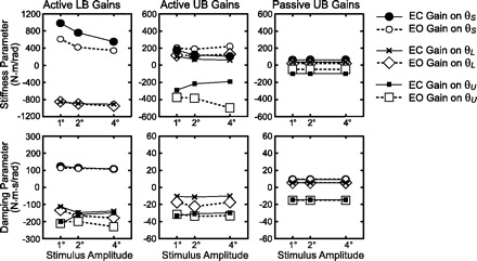
LB and UB stance control systems represented by the stiffness and damping parameter values from Figs. 3 and 4 transformed into gains on state variables θL and θU and their derivatives and gains representing the coupling of the stimulus, θS, to balance control.
For UB active control, the restructured model representation (Fig. 5, middle) demonstrates a large coupling of both surface tilt (but only through the stiffness factor and not the damping factor) and LB motion to UB control. The surface-tilt coupling is masked in the Fig. 1 model representation because there is no sensory input to the active UB control mechanism that is a direct sensory representation of θS. Rather, the surface-tilt coupling to UB control occurs through the sensory input encoding θP − θU, because θP is a function of θL and θS (Appendix, Eq. A4).
Only intrinsic mechanisms.
One simple control hypothesis is that the LB and UB system is based entirely on passive mechanisms. That is, LB control is based on passive stiffness and damping factors that orient the LB toward the surface with no time delay, and UB control is based on passive stiffness and damping factors that orient the UB toward the pelvis with no time delay. To determine the extent to which passive mechanisms could account for the experimental data, only KUi, BUi, KLi, and BLi were allowed to be nonzero in the Fig. 1 model. Results from a model based on passive mechanisms were only able to account for some of the general features of experimental FRF gains (Fig. 6A, red curves). UB phase curves were poorly described. Only with a large decrease in damping could UB phases be better accounted for, but a decrease in damping also produced high-resonance peaks in gain curves and therefore no overall improvement. Similarly, the model-predicted IRFs did not describe the experimental data well (Fig. 6B). However, the very early time course (<50 ms) of UB IRFs was similar to experimental UB IRFs, indicating the importance of passive mechanisms in determining the early time course of UB IRFs.
Only active sensory feedback.
A model structure was also explored where control was based entirely on active sensory feedback mechanisms (i.e., KUi, BUi, KLi, and BLi were all set to zero). The model predictions were dependent on sensory feedback time delays (τL and τU). When τL and τU were both set to 100 ms, the optimization routine failed to find parameters associated with stable control. When τL and τU were set to 117 and 84 ms, respectively (based on fits to mean FRFs), the optimization routine also failed to find parameters associated with stable control. When τU was reduced to 50 ms, stable control could be achieved and the experimental FRFs were well described over most of the frequency range (Fig. 6A, blue curves). However, the early time courses of LB and UB IRFs were not well described by the model with only active feedback (Fig. 6B). Specifically, the model-predicted IRFs exhibited a clear delay that was not present in the experimental data, followed by an overshoot of the experimental IRFs.
Absent torque feedback.
The influence of torque feedback was also explored by setting the torque feedback gain (GLt) to zero and observing the predicted FRFs in narrow stance conditions (Fig. 6A). Without torque feedback in the LB control system, model-predicted FRF gains in both the LB and UB were too high and phases were too low at frequencies less than ∼0.15 Hz. Thus model results showed that torque feedback primarily influenced low frequencies by reducing UB and LB gains and by enhancing UB and LB phase leads.
Future Model Refinement
There a several ways the model could be used in future studies to obtain more insight into the balance control system. Because the model represented the contribution of specific sensory systems to balance control, quantitative model predictions could be tested by performing experiments on subjects with sensory loss in particular systems. Also, the model could be used to explore whether optimization principles can account for the experimentally observed dynamic behavior and sensory reweighting (Goodworth et al. 2009; Kuo 1995, 2005; Qu and Nussbaum 2009; van der Kooij and Peterka 2011).
GRANTS
This work was supported by National Institute on Aging Grant AG17960.
DISCLOSURES
No conflicts of interest, financial or otherwise, are declared by the author(s).
AUTHOR CONTRIBUTIONS
A.D.G. and R.J.P. conception and design of research; A.D.G. and R.J.P. performed experiments; A.D.G. and R.J.P. analyzed data; A.D.G. and R.J.P. interpreted results of experiments; A.D.G. and R.J.P. prepared figures; A.D.G. and R.J.P. drafted manuscript; A.D.G. and R.J.P. edited and revised manuscript; A.D.G. and R.J.P. approved final version of manuscript.
APPENDIX
Description and Simplification of Body Mechanics
Figure A1A shows a schematic of a frontal plane multisegment body with the LB represented as a closed-chain mechanical system. The UB representation is a simplification of the true mechanics in that the pelvis-UB joint was assumed to be located at the midpoint between hip joint centers. This simplification means that the pelvis-UB joint location at any point in time is influenced only by θL. A more anatomically accurate model would include the distance between hip joint centers and the L4/L5 joint, which would result in a pelvis-UB joint position that is influenced by θP, which is a function of both θS and θL. This pelvis-UB joint simplification was previously shown to affect the early time course (<50 ms) of UB IRFs (Fig. 3 in Goodworth and Peterka 2009) via additional interaction torques associated with lateral displacements of the pelvis-UB joint as a function of θS, but otherwise did not influence the IRFs.
Fig. A1.
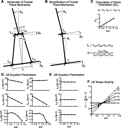
Multisegment mechanical models of LB and UB frontal plane mechanics. Schematics are shown of a full mechanical system (A) with LB closed-chain mechanical linkage and a simplified system (B) defined by UB orientation (θU), LB orientation (θL), pelvis orientation (θP), support surface tilt angle (θS), LB torque (TL), and UB torque (TU). The pelvis ratio (PR) parameter (defined in C) was used in Eq. A4 to determine θP as a function of θS and θL. LB mechanical parameters (D) were used in Eq. A1, and UB mechanical parameters (E) were used in Eq. A2. The R factor (defined in F) was used in Eq. A1 to scale TL. All plots show parameter variations as a function of the ratio of heel-to-heel stance width (S) to the distance between hip joint centers (W). Parameters were evaluated at S/W values of 0, 0.63, 1.03, 1.57, and 2.11, which correspond to intermalleolar distances of 0, 5, 12, 21.5, and 31 cm, respectively, for our average subject. LB and UB parameters shown represent values based on the mean body mass and dimensions of subjects in the study.
Following the approach of Koozekanani et al. 1980, equations of motion in the frontal plane were calculated for the Fig. A1A system by developing free body diagrams (D'Alembert's principle) of the surface, two legs, a pelvis, and a UB in an earth-fixed Cartesian coordinate system, where the left ankle was assumed to be the origin. Three equations (one force equation with respect to earth horizontal, one force equation with respect to earth vertical, and one moment equation) were developed for each segment, resulting in a total of 15 free body diagram equations. The free body diagram equations were solved simultaneously using the Symbolic Math Toolbox in Matlab (The MathWorks) so that LB and UB torque was related to segment motion (position, velocity, and acceleration) and segment dimensions (mass, length, CoM location, moments of inertia, and stance width). Equations were solved separately for each subject and for an average subject based on mean segment dimensions.
The equations of motion for the Fig. A1A model are extremely complex due to the closed-chain mechanics of the LB. We sought a more tractable two-segment inverted pendulum mechanical model representation by recognizing that although the LB consists of two leg segments and one pelvis segment, the LB has only one degree of freedom in the frontal plane (assuming straight knees), because the two legs and pelvis form a closed loop system (Day et al. 1993). To formulate a two-segment approximation to the mechanical system in Fig. A1A, the LB and UB equations of motion were linearized about the vertical orientation. The schematic in Fig. A1B shows the linearized system represented as a two-segment inverted-pendulum. The equations of motion for this two-segment representation are
| (A1) |
| (A2) |
with
| (A3) |
In Eqs. A1 and A2, TL is the torque applied to the LB segment at an equivalent ankle joint and is equal to the sum of torques applied to the two ankle and two hip joints, TU is the torque applied to the UB segment, g is the acceleration due to gravity, J parameters are factors related to inertial torques, and A parameters are factors related to torques due to gravity. Unlike an actual two-segment inverted pendulum, all six of the J and A parameters in Eq. A1 vary as a function of the ratio of stance width, S, to hip width, W (Fig. A1D). These parameters' variations with S/W account for the fact that, in the LB closed-chain mechanical system represented in Fig. A1A, when a given joint torque is applied at an ankle or hip joint, the angular acceleration of the LB depends not only on the magnitude of the applied torque but also on the configuration of the LB mechanical system as defined by S/W (Bingham et al. 2011). In addition to J and A parameters varying with S/W in Eq. A1, the effectiveness of TL depends on S/W and on the distribution, D, of TL between hip and ankle joints with D being equal to the proportion of TL applied to the hip joints. The scale factor R (Eq. A3), which multiplies TL in Eq. A1, defines how S/W and D influence the effectiveness of TL. Figure A1F shows how R varies as a function of S/W for various values of D. In the current study, the average subject S/W was 0.63, and we assumed that TL was distributed equally among the four LB joints, giving D = 0.5. Thus R = 0.82 for the average subject.
As S approaches zero, the LB effectively becomes a fixed triangular structure where the hip angle cannot change, and Eqs. A1 and A2 become equivalent to previously published equations for a two-segment inverted pendulum (e.g., Eq. 6.58 in Craig 1989). In the UB equation of motion (Eq. A2), JUL varied only minimally with S/W, and JU and AU did not vary with S/W (Fig. A1E). Note that previously published two-segment (Kiemel et al. 2008) and multisegment inverted pendulum equations (Koozekanani et al. 1983) use a different equation form that includes terms that are the difference between adjacent joint torques. For example, an alternative version of Eq. A1 could be written that includes TL − TU on the right side of the equation. This equation form can be converted to the form we used by solving Eq. A2 for TU and then substituting for TU in the alternative version of Eq. A1 to give our version of Eq. A1, which includes only TL.
To determine the accuracy of the linearized equations, we compared LB and UB torques predicted from the linearized equations with torques predicted from the full solution for each test condition. For the linearized set of equations, θS, θL, and θU positions and accelerations from the mean experimental time series over the 43.72-s cycle duration were substituted into Eqs. A1 and A2 to calculate TL and TU using the appropriate coefficients from Fig. A1, D and E, for each test condition. Similarly, for the full set of 15 equations, θS, θL, and θU position, velocity, and accelerations from the mean experimental time series were used to calculate TL and TU. The comparison of TL and TU time series from the linearized and full equations showed excellent agreement [R2 values of nearly 1 (>0.999) across all test conditions]. Therefore, the linearized equations provided an accurate description of body dynamics over the range of experimentally obtained LB and UB sway.
Description of Pelvis Tilt Angle
An important mechanical feature of frontal plane body mechanics that is not captured by the two-segment body model alone is the orientation angle of the pelvis, θP, as a function of LB sway and surface tilt. Although θP does not appear in Eqs. A1 and A2, θP is a potentially important kinematic variable, since previous results demonstrated that a proprioceptive signal encoding θP − θU contributed to UB control (Goodworth and Peterka 2009).
The simplified frontal plane mechanical model is completed by defining how θP varies as a function of θL and θS. The exact relationship of θP to θL and θS is a complex trigonometric function that depends on S/W, but at a given S/W, a simple linear approximation provides a satisfactory representation over the range of θS and θL values found in the experimental data. The linear approximation was obtained by calculating an exact set of θP, θL, and θS angles at a given S/W and then fitting the following equation to this data set:
| (A4) |
where the “pelvis ratio” parameter, PR (which depends on S/W) is the only parameter needed to define θP as a function of θL and θS.
To obtain the exact θP, θL, and θS angles needed to derived the PR parameter in Eq. A4, we used the trigonometric equations of Day et al. (1993) to define the LB ankle and hip joint angles. Because all LB joint angles are determined once any single LB joint angle is specified, we varied one ankle angle relative to θS between ±2° in 0.1° increments to calculate a range of ankle and hip angles compatible with the range in experimental data. For each incremented ankle angle, the set of ankle and hip joint angles and the known segment lengths were used to determine the coordinates of hip joint centers and the midpoint between the hip joint centers. The hip joint center coordinates were used to calculate θP, and the hip midpoint coordinates were used to calculate θL. This procedure was repeated for θS angles between ±2° in 0.1° increments to obtain a set of exact θP, θL, and θS angles, at a given S/W, needed to obtain the value of PR. Four stance widths were evaluated with their PR values shown in Fig. A1C. The linear approximation provided an excellent representation of θP as a function of θL and θS [minimum R2 value of nearly 1 (>0.999) between the full trigonometric calculation of θP and the calculation of θP using the Eq. A4 approximation across 4 stance widths of 5-, 12-, 21.5-, and 31-cm intermalleolar distances (IMDs), corresponding to S/W values of 0.63, 1.03, 1.57, and 2.11 for our average subject].
The PR values in Fig. A1C show that when heel-to-heel distance is equal to the distance between hip joint centers (S/W = 1 at ∼12-cm IMD), PR = 1 and θP = θS (Fig. A1C). For S/W < 1, PR is less than one and positive θS and θL values both result in positive values of θP. However, for S/W > 1, PR is greater than one and positive θS gives positive θP while positive θL gives negative θP values.
Interpretation of LB Control Parameters
Our model analysis assumed that LB torque was generated equally across all four LB joints (D = 0.5). However, an identical LB segmental motion can occur with an appropriately scaled torque generated about only one LB joint or about any combination of joints (Bingham et al. 2011). With this type of system, it is likely that the proportion of torque generation about one joint compared with another is dictated by optimization principles so that some cost function is minimized (e.g., Todorov 2004). However, it was beyond the scope of the current study to investigate the optimal distribution of LB torque. Instead, the current study focused on identifying contributions to TL, the summation of all passive and active mechanisms that generate LB torque applied equally about all LB joints (Fig. A1B). The assumption that LB torque was generated equally across all LB joints was chosen for simplicity and was arbitrary. Had a different assumption been made about which LB joint or joints torque was applied, determination of all UB parameters, the LB time delay (τL), and the time constant of torque feedback (τLt) would have been unaffected, but the remaining LB control parameters would need to have been scaled to different values to accommodate the different assumption. The following discussion focuses on these remaining LB control parameters and does not pertain to LB parameters τL and τLt, or to any UB parameters.
The relationship among LB joint torques is particularly simple in the condition where the LB forms a parallelogram, because a given torque applied at a particular LB joint results in identical segmental motion as if the torque were applied at any one of the other three LB joints (S = W, and therefore R = 1 for all values of D; see Eq. A3 and Fig. A1F). Consequently, there is no need to adjust LB feedback parameters to account for different assumptions about how the total LB torque is distributed among the LB joints.
At other stance widths, torque applied about an ankle joint results in different LB motion from that which would have occurred if the same torque was applied about a hip joint. Specifically, for S/W < 1, ankle torque is more effective than hip torque; and vice versa for S/W > 1. Thus the interpretation of variations in LB control parameter values with varying stimulus amplitude at a particular stance width is complicated by the fact that the torque distribution between ankle and hip influences LB motion at stance widths other than when the LB forms a parallelogram. For example, in an EC narrow stance condition addressed in the present study, KLl increased with increasing stimulus amplitude (Fig. 3B, left). This increase could represent a change in the LB balance control where 1) the proportional distribution of total LB torque among the ankle and hip joints remained fixed and the muscle activations generating torque at the ankle and hip joints all increased with increasing stimulus amplitude; 2) there was a redistribution of total LB torque among the ankle and hip joints such that there was an increase in the proportion of torque applied to the ankle joints relative to torque applied to hip joints (i.e., when S/W < 1, a decrease in D causes an increase in R and, therefore, an increased effectiveness of TL; see Fig. A1F); or 3) there was a combination of an increased torque generation at ankle and hip joints as well as a redistribution of joint torques that increased the proportions of ankle torque relative to hip torque. In all cases, the change in KLl across stimulus amplitude or between EO and EC conditions indicates there were neurally mediated changes in the active LB control mechanism that altered the dynamic characteristics of the LB, but the changes in KL1 do not specify the exact method the nervous system used to achieve the change in LB control. The same considerations apply to the other LB stiffness and damping parameters.
REFERENCES
- Alexandrov AV, Frolov AA, Horak FB, Carlson-Kuhta P, Park S. Feedback equilibrium control during human standing. Biol Cybern 93: 309–322, 2005 [DOI] [PMC free article] [PubMed] [Google Scholar]
- Allison LK, Kiemel T, Jeka JJ. Multisensory reweighting of vision and touch is intact in healthy and fall-prone older adults. Exp Brain Res 175: 342–352, 2006 [DOI] [PubMed] [Google Scholar]
- Angelaki DE, McHenry MQ, Dickman JD, Newlands SD, Hess BJ. Computation of inertial motion: Neural strategies to resolve ambiguous otolith information. J Neurosci 19: 316–327, 1999 [DOI] [PMC free article] [PubMed] [Google Scholar]
- Barin K. Evaluation of a generalized model of human postural dynamics and control in the sagittal plane. Biol Cybern 61: 34–50, 1989 [DOI] [PubMed] [Google Scholar]
- Bendat JS, Piersol AG. Random Data: Analysis and Measurement Procedures. New York: Wiley, 2000 [Google Scholar]
- Bingham JT, Choi JT, Ting LH. Stability in a frontal plane model of balance requires coupled changes to postural configuration and neural feedback control. J Neurophysiol 106: 437–448, 2011 [DOI] [PMC free article] [PubMed] [Google Scholar]
- Bosco G, Poppele RE. Broad directional tuning in spinal projections to the cerebellum. J Neurophysiol 70: 863–866, 1993 [DOI] [PubMed] [Google Scholar]
- Bosco G, Poppele RE, Eian J. Reference frames for spinal proprioception: limb endpoint based or joint-level based? J Neurophysiol 83: 2931–2945, 2000 [DOI] [PubMed] [Google Scholar]
- Casabona A, Stella Valle M, Bosco G, Perciavalle V. Cerebellar encoding of limb position. Cerebellum 3: 172–177, 2004 [DOI] [PubMed] [Google Scholar]
- Cenciarini M, Peterka RJ. Stimulus-dependent changes in the vestibular contribution to human postural control. J Neurophysiol 95: 2733–2750, 2006 [DOI] [PubMed] [Google Scholar]
- Cordo PJ, Nashner LM. Properties of postural adjustments associated with rapid arm movements. J Neurophysiol 47: 287–302, 1982 [DOI] [PubMed] [Google Scholar]
- Craig JJ. Introduction to Robotics: Mechanics and Control (2nd ed.). New York: Addison-Wesley, 1989 [Google Scholar]
- Davies WDT. System Identification for Self-Adaptive Control. New York: Wiley-Interscience, 1970 [Google Scholar]
- Day BL, Steiger MJ, Thompson PD, Marsden CD. Effect of vision and stance width on human body motion when standing: implications for afferent control of lateral sway. J Physiol 469: 479–499, 1993 [DOI] [PMC free article] [PubMed] [Google Scholar]
- Erdmann WS. Geometric and inertial data of the trunk in adult males. J Biomech 30: 679–688, 1997 [DOI] [PubMed] [Google Scholar]
- Ernst MO, Banks MS. Humans integrate visual and haptic information in a statistically optimal fashion. Nature 415: 429–433, 2002 [DOI] [PubMed] [Google Scholar]
- Goodworth AD, Peterka RJ. Contribution of sensorimotor integration to spinal stabilization in humans. J Neurophysiol 102: 496–512, 2009 [DOI] [PMC free article] [PubMed] [Google Scholar]
- Goodworth AD, Peterka RJ. Influence of bilateral vestibular loss on spinal stabilization in humans. J Neurophysiol 103: 1978–1987, 2010a [DOI] [PMC free article] [PubMed] [Google Scholar]
- Goodworth AD, Peterka RJ. Influence of stance width on frontal plane postural dynamics and coordination in human balance control. J Neurophysiol 104: 1103–1118, 2010b [DOI] [PMC free article] [PubMed] [Google Scholar]
- Goodworth AD, Wall C, III, Peterka RJ. Influence of feedback parameters on performance of a vibrotactile balance prosthesis. IEEE Trans Neural Syst Rehabil Eng 17: 397–409, 2009 [DOI] [PMC free article] [PubMed] [Google Scholar]
- Henry SM, Fung J, Horak FB. EMG responses to maintain stance during multidirectional surface translations. J Neurophysiol 80: 1939–1950, 1998 [DOI] [PubMed] [Google Scholar]
- Kiemel T, Elahi AJ, Jeka JJ. Identification of the plant for upright stance of humans: multiple movement patterns from a single neural strategy. J Neurophysiol 100: 3394–3406, 2008 [DOI] [PMC free article] [PubMed] [Google Scholar]
- Koozekanani SH, Stockwell CW, McGhee RB, Firoozmand F. On the role of dynamic models in quantitative posturography. IEEE Trans Biomed Eng 27: 605–609, 1980 [DOI] [PubMed] [Google Scholar]
- Koozekanani SH, Barin K, McGhee RB, Chang HT. A recursive free-body approach to computer simulation of human postural dynamics. IEEE Trans Biomed Eng 30: 787–792, 1983 [DOI] [PubMed] [Google Scholar]
- Kuo AD. An optimal control model for analyzing human postural balance. IEEE Trans Biomed Eng 42: 87–101, 1995 [DOI] [PubMed] [Google Scholar]
- Kuo AD. An optimal state estimation model of sensory integration in human postural balance. J Neural Eng 2: S235–S249, 2005 [DOI] [PubMed] [Google Scholar]
- Maurer C, Mergner T, Peterka RJ. Multisensory control of human upright stance. Exp Brain Res 171: 231–250, 2006 [DOI] [PubMed] [Google Scholar]
- Merfeld DM, Zupan LH. Influence of rotational cues on the neural processing of gravito-inertial force. In: Levels of Perception, edited by Harris LR, Jenkin M. New York: Springer, 2003, p. 351–384 [Google Scholar]
- Mergner T. A neurological view on reactive human stance control. Annu Rev Control 34: 177–198, 2010 [Google Scholar]
- Mergner T, Hlavacka F, Schweigart G. Interaction of vestibular and proprioceptive inputs. J Vestib Res 3: 41–57, 1993 [PubMed] [Google Scholar]
- Mergner T, Huber W, Becker W. Vestibular-neck interaction and transformation of sensory coordinates. J Vestib Res 7: 347–367, 1997 [PubMed] [Google Scholar]
- Mergner T, Rosemeier T. Interaction of vestibular, somatosensory and visual signals for postural control and motion perception under terrestrial and microgravity conditions - a conceptual model. Brain Res Rev 28: 118–135, 1998 [DOI] [PubMed] [Google Scholar]
- Mergner T, Siebold C, Schweigart G, Becker W. Human perception of horizontal trunk and head rotation in space during vestibular and neck stimulation. Exp Brain Res 85: 389–404, 1991 [DOI] [PubMed] [Google Scholar]
- Oie KS, Kiemel T, Jeka JJ. Multisensory fusion: simultaneous re-weighting of vision and touch for the control of human posture. Cogn Brain Res 14: 164–176, 2002 [DOI] [PubMed] [Google Scholar]
- Park S. Human Standing Postural Control Adjusts to Biomechanical Constraints (PhD thesis). Ann Arbor, MI: University of Michigan, 2002 [Google Scholar]
- Park S, Horak FB, Kuo AD. Postural feedback responses scale with biomechanical constraints in human standing. Exp Brain Res 154: 417–427, 2004 [DOI] [PubMed] [Google Scholar]
- Peterka RJ. Sensorimotor integration in human postural control. J Neurophysiol 88: 1097–1118, 2002 [DOI] [PubMed] [Google Scholar]
- Peterka RJ. Simplifying the complexities of maintaining balance. IEEE Eng Med Biol Mag 22: 63–68, 2003 [DOI] [PubMed] [Google Scholar]
- Peterka RJ, Loughlin PJ. Dynamic regulation of sensorimotor integration in human postural control. J Neurophysiol 91: 410–423, 2004 [DOI] [PubMed] [Google Scholar]
- Pintelon R, Schoukens J. System Identification: A Frequency Domain Approach. Piscataway, NJ: IEEE, 2001 [Google Scholar]
- Qu X, Nussbaum MA. Evaluation of the roles of passive and active control of balance using a balance control model. J Biomech 42: 1850–1855, 2009 [DOI] [PubMed] [Google Scholar]
- Scrivens JE, DeWeerth SP, Ting LH. A robotic device for understanding neuromechanical interactions during standing balance control. Bioinsp Biomim 3: 026002, 2008 [DOI] [PubMed] [Google Scholar]
- Seidel GK, Marchinda DM, Dijkers M, Soutas-Little RW. Hip joint center location from palpable bony landmarks—a cadaver study. J Biomech 28: 995–998, 1995 [DOI] [PubMed] [Google Scholar]
- Skotte JH. Estimation of low back loading on nurses during patient handling tasks: the importance of bedside reaction force measurement. J Biomech 34: 273–276, 2001 [DOI] [PubMed] [Google Scholar]
- Todorov E. Optimality principles in sensorimotor control. Nat Neurosci 7: 907–915, 2004 [DOI] [PMC free article] [PubMed] [Google Scholar]
- van der Kooij H, Jacobs R, Koopman B, Grootenboer H. A multisensory integration model of human stance control. Biol Cybern 80: 299–308, 1999 [DOI] [PubMed] [Google Scholar]
- van der Kooij H, Jacobs R, Koopman B, van der Helm F. An adaptive model of sensory integration in a dynamic environment applied to human stance control. Biol Cybern 84: 103–115, 2001 [DOI] [PubMed] [Google Scholar]
- van der Kooij H, Peterka RJ. Non-linear stimulus-response behavior of the human stance control system is predicted by optimization of a system with sensory and motor noise. J Comput Neurosci 30: 759–778, 2011 [DOI] [PMC free article] [PubMed] [Google Scholar]
- Westwick DT, Kearney RE. Identification of Nonlinear Physiological Systems. Piscataway, NJ: Wiley-Interscience, 2003 [Google Scholar]
- Winter DA. Biomechanics and Motor Control of Human Movement. Hoboken, NJ: Wiley, 2005 [Google Scholar]