

Abstract
Correlations between spontaneous fluctuations in the blood oxygenation level dependent (BOLD) signal measured with functional MRI are finding increasing use as measures of functional connectivity in the brain, where differences can potentially predict cognitive performance and diagnose disease. Caffeine, which is a widely consumed neural stimulant and vasoactive agent, has been found to decrease the amplitude and correlation of resting-state BOLD fluctuations, and hence is an important factor to consider in functional connectivity studies. However, because the BOLD signal is sensitive to neural and vascular factors, the physiological mechanisms by which caffeine alters spontaneous BOLD fluctuations remain unclear. Resting-state functional connectivity has traditionally been assessed using stationary measures, such as the correlation coefficient between BOLD signals measured across the length of a scan. However, recent work has shown that the correlation of resting-state networks can vary considerably over time, with periods as short as 10 seconds. In this study, we used a sliding window correlation analysis to assess temporal variations in resting-state functional connectivity of the motor cortex before and after caffeine ingestion. We found that the temporal variability of BOLD correlation was significantly higher following a caffeine dose, with transient periods of strong correlation alternating with periods of low or negative correlation. This phenomenon was primarily due to increased variability in the phase difference between BOLD time courses in the left and right motor cortices. These results indicate that caffeine may cause underlying spontaneous neural fluctuations to go in and out of coherence more frequently, and emphasizes the need to consider non-stationary measures when studying changes in functional connectivity.
Keywords: nonstationary, functional MRI, resting-state network, temporal dynamics, correlation, spectral decomposition
Introduction
Resting-state functional MRI (fMRI) can be used to assess functional connectivity within the brain through the measurement of correlations between spontaneous blood oxygenation level-dependent (BOLD) fluctuations in different regions. Synchronous BOLD fluctuations have been consistently found at rest within functional networks such as the motor cortex, visual cortex, and default mode network (DMN) (Biswal et al. 1995; Lowe et al. 1998; Greicius et al. 2003). A growing number of studies have shown that functional connectivity is altered for cognitive disorders such as multiple sclerosis, epilepsy, Parkinson’s, and Alzheimer’s disease (Lowe et al. 2002; Greicius et al. 2004; Lui et al. 2008; Kwak et al. 2010), suggesting that resting-state studies can aid in disease diagnosis and improved understanding of disease mechanisms. In addition, inter-subject differences in functional connectivity have been shown to correlate with performance on working memory tasks and intelligence (Hampson et al. 2006; Song et al. 2008).
To date, functional connectivity studies have typically employed stationary metrics obtained with seed-based correlations or independent component analysis computed over an entire resting scan. However, recent work has shown that the correlation strength between different brain regions may vary in time. For example, a study using magnetoencephalography (MEG) found transient formations of widespread correlations in resting-state power fluctuations within the DMN and task positive network (TPN) (de Pasquale et al. 2010). This nonstationary phenomenon was particularly apparent when considering nodes in different hemispheres, which exhibited very low stationary correlation. Another study using fMRI found that the phase angle between spontaneous BOLD fluctuations in the DMN and TPN varied considerably over time, with frequent periods of significant anti-correlation (Chang and Glover 2010). These studies indicate that coordination of spontaneous neural activity is a dynamic process, and suggest that time varying approaches can provide critical insights into functional connectivity.
Despite the increasing appearance of resting-state functional connectivity studies in the literature, it remains difficult to interpret the physiological mechanisms behind changes in BOLD signal correlations. The BOLD signal provides an indirect measure of neural activity, and is a complex function of changes in cerebral blood flow (CBF), cerebral blood volume, and oxygen metabolism (Buxton et al. 2004). Factors that alter any part of the pathway between neural activity and the BOLD response can change functional connectivity measurements, making it difficult to decipher the origin of this effect. For example, caffeine is a widely used stimulant that has a complex effect on the coupling between neural activity and blood flow (Fredholm et al. 1999; Pelligrino et al. 2010). Through adenosine antagonism, caffeine enhances neural activity by blocking the inhibitory affects of adenosine activation (Dunwiddie and Masino 2001). In addition, by inhibiting adenosine binding to receptors on smooth muscles cells, caffeine reduces the ability of blood vessels to dilate (Meno et al. 2005; Pelligrino et al. 2010) and causes an overall reduction in baseline cerebral blood flow (Cameron et al. 1990). All of these factors can lead to BOLD signal changes.
Previous work by our group assessing caffeine’s effect on resting-state BOLD fluctuations has shown that it reduces both the stationary correlation and amplitude of the fluctuations in the motor cortex (Rack-Gomer et al. 2009). While it is difficult to determine the underlying physiological mechanisms behind this effect, recent studies suggests that it may stem primarily from changes in neural activity coherence. For example, preliminary work by our group with magnetoencephalography (MEG) found similar reductions in the correlation of MEG power fluctuations in the motor cortex, which do not have the same vascular confounds that are present in the BOLD fMRI signal (Tal et al. 2011). In addition, caffeine has been shown to impair motor learning compared to a placebo (Mednick et al. 2008). Since it has been shown that the strength of resting-state functional connectivity is related to memory performance (Hampson et al. 2006), these findings suggest that the caffeine-induced reduction in BOLD correlation may represent underlying neural changes.
In this study, we employed a non-stationary analysis approach to gain further insight into the mechanisms of caffeine’s effect on functional connectivity. Specifically, we used a sliding window correlation analysis to assess whether caffeine consistently weakens the correlation over time or if transient periods of strong correlation still exist, albeit less frequently. A persistent and stationary decrease in correlation could be caused by an overall change in the vascular system induced by caffeine. However, it is unlikely that a shift in the state of the vascular system would give rise to an increase in the non-stationarity of the correlations, when viewed on a time scale of tens of seconds. Instead, a caffeine-induced increase in the temporal variability of the correlations would tend to support the existence of greater temporal variability in the coherence of the underlying neural fluctuations.
Methods
Experimental protocol
The data used in this study were collected for a previous experiment examining the effects of caffeine on resting-state BOLD connectivity as assessed with stationary correlation measures (Rack-Gomer et al. 2009). Nine healthy volunteers (5 males and 4 females, ages 23 to 41 years) participated in this study after providing informed consent. Participants were instructed to refrain from ingesting caffeine for at least 12 hours prior to being scanned. The estimated daily caffeine usage for each subject based on self-reports of coffee, tea, and soda consumption is presented in Table 1. The assumed caffeine contents for an 8-oz cup of coffee, an 8-oz cup of tea, and a 12-oz soda were 100 mg, 40 mg, and 20 mg respectively (Fredholm et al. 1999).
Table 1.
Estimated daily caffeine usage and the number of voxels in each ROI for each subject. The volume of each voxel is 84.4 mm3.
| Subject | Estimated daily caffeine usage (mg) | Volume of Right ROI (voxels) | Volume Left ROI (voxels) |
|---|---|---|---|
| 1 | < 30 | 31 | 9 |
| 2 | < 30 | 10 | 10 |
| 3 | 340 | 12 | 25 |
| 4 | < 30 | 12 | 7 |
| 5 | 50 | 30 | 35 |
| 6 | < 30 | 36 | 27 |
| 7 | 50 | 28 | 23 |
| 8 | < 30 | 11 | 25 |
| 9 | 225 | 25 | 21 |
Each subject participated in two imaging sessions: a caffeine session and a control session, in that order. The two imaging sessions were separated by at least 6 weeks. The caffeine session consisted of a pre-dose and a post-dose imaging section, each lasting around 45 minutes. Upon completion of the pre-dose section, participants ingested a 200 mg caffeine pill and then rested for approximately 30 minutes outside of the magnet before starting the post-dose section. The first resting-state scan of the post-dose section began approximately 45 minutes after the caffeine pill was ingested to achieve approximately 99% absorption of caffeine from the gastrointestinal tract (Fredholm et al. 1999). Control sessions used the same protocol, but without the administration of caffeine between sections, similar to the protocol used in (Perthen et al. 2008). Subjects were not given a placebo during the control session. However, for convenience, we will still refer to the two scan sections as the “pre-dose” and “post-dose” sections.
Each scan section included a high-resolution anatomical scan, a bilateral finger tapping block design, and two five-minute resting-state BOLD scans. Bilateral finger tapping was self-paced and the block design run consisted of 20s rest followed by 5 cycles of 30s tapping and 30s resting. Subjects were instructed to tap while a flashing checkerboard was displayed and then to rest during the display of a control image, consisting of a white square situated in the middle of a gray background. During resting-state scans, the control image was displayed for the entirety of the scan and subjects were asked to maintain attention on the white square.
Image acquisition
Imaging data were collected on a GE Excite HDX 3 Tesla whole body system with an eight channel receive coil. Laser alignment was used to landmark subjects and minimize differences in head position between pre-dose and post-dose sections.
The high-resolution anatomical scan was acquired with a magnetization prepared 3D fast spoiled gradient (FSPGR) sequence (TI=450 ms, TR=7.9 ms, TE=3.1 ms, 12° flip angle, FOV 25 cm, 256 × 256 matrix, slice thickness = 1mm). Functional data were collected over six oblique 6-mm thick slices prescribed through the primary motor cortex. The finger tapping scan was acquired with a PICORE QUIPSS II (Wong et al. 1998) arterial spin labeling (ASL) sequence (TR = 2s, TI1/TI2 = 600/1500 ms, 10 cm tag thickness, 1 cm tag-slice gap) with dual echo spiral readout (TE1/TE2 = 9.2/30 ms, FOV = 24 cm, 64 × 64 matrix, and flip angle = 90°). The two resting-state BOLD scans were acquired using BOLD-weighted imaging with spiral readout (TE = 30 ms, TR = 500 ms, FOV = 24 cm, 64 × 64 matrix, and flip angle = 45°).
Cardiac pulse and respiratory effort data were monitored using a pulse oximeter (InVivo) and a respiratory effort transducer (BIOPAC), respectively. The pulse oximeter was placed on the subject’s index finger, and the respiratory effort belt was placed around the subject’s abdomen. The pulse oximeter was not worn during the bilateral finger-tapping scan. Physiological data were sampled at 40 samples per second using a multi-channel data acquisition board (National Instruments).
Data analysis
Images from each scan section were co-registered using AFNI software (Cox 1996). In addition, the anatomical volume from each post-dose section was aligned to the anatomical volume of its respective pre-dose section, and the rotation and shift matrix used for this alignment was then applied to the post-dose functional images. The outer two slices of the functional data were discarded to minimize partial volume effects associated with the rotation of the post-dose data, and the first 10s of each functional run were not included. In addition, voxels from the edge of the brain were not included in the analysis in order to minimize the effects of motion.
The second echo data from the finger tapping scans were used to generate BOLD activation maps of the motor cortex. This was accomplished using a general linear model (GLM) approach for the analysis of ASL data (Mumford et al. 2006; Restom et al. 2006). The stimulus-related regressor was produced by the convolution of the square wave stimulus pattern with a gamma density function (Boynton et al. 1996). Constant and linear trends were included in the GLM as nuisance regressors. In addition, the data were pre-whitened using an autoregressive model of order 1 (Burock and Dale 2000; Woolrich et al. 2001). The statistical maps were based on the square root of the F-statistic, which is equal to the t-statistic in the case of one nuisance term (Liu et al. 2001). For consistency with our prior study (Rack-Gomer et al. 2009), active voxels were defined using a method based on activation mapping as a percentage of local excitation (AMPLE) (Voyvodic 2006). In summary, the maps were separated into left and right hemispheric regions. The highest value in each region was identified and then every voxel was converted to a percentage of the peak statistical value for the region ( ). Active voxels were required to exceed an AMPLE value of 45% and a value of 2 (p < 0.05). The final activation maps were defined from the intersection of voxels active in both pre-dose and post-dose scan sections. Regions of interest (ROIs) were then defined for the left and right motor cortices from these activation maps. Thus, the same ROIs were used in the comparison of pre-dose and post-dose functional connectivity within an imaging session. The numbers of voxels in each subject’s left and right ROIs are listed in Table 1.
Nuisance terms were removed from the BOLD resting-state data through linear regression. Nuisance regressors included constant and linear trends, 6 motion parameters obtained during image co-registration, physiological noise contributions (Glover et al. 2000), low frequency variations in cardiac and respiratory rate (Birn et al. 2008; Chang et al. 2009), and a version of the global signal that we will call the “regional” signal term. The regional signal term was calculated as the mean signal from the anterior portion of the brain in order to minimize bias that can occur when all the voxels in the brain are used to define a global mean signal as a nuisance regressor (Murphy et al. 2009). Data were then temporally low-pass filtered using a finite impulse response function (Diniz et al. 2002) with a cutoff frequency of 0.08 Hz. This cutoff frequency was chosen for consistency with previous functional connectivity studies (Biswal et al. 1997; Cordes et al. 2001; Fox et al. 2005).
To quantify functional connectivity strength, we extracted average BOLD signals from the left and right motor cortices. A stationary measure of inter-hemispheric functional connectivity was calculated as the correlation coefficient between the right and left motor BOLD signals computed over the entire length of each resting run. To assess temporal variations in inter-hemispheric motor cortex connectivity, we applied a sliding window over the length of each resting run and calculated the correlation between the left and right motor BOLD signals within each window. Correlation variability was quantified as the standard deviation of the sliding window correlation time series. To assess the affect of window length on correlation variability, we varied the window length from 10 seconds to 100 seconds in 1 second increments.
For all subjects, metrics were averaged across the two resting runs in each scan section. Two-tailed paired t-tests were performed between the pre-dose and post-dose results to assess caffeine-induced changes. In addition, a repeated measures two-way analysis of variance (ANOVA) was performed for each metric to assess the interaction between caffeine and scan session.
Cross Power Analysis
To gain more insight into the cause of temporal variations in BOLD signal correlation, we performed a cross power analysis on each pair of left and right motor cortex BOLD signals. Let x[n] and y[n] represent the average BOLD time courses from the left and right motor cortices, respectively. The power spectral estimate of x[n], which is of length N and sampled at a rate of fs, is given by
| (1) |
where horizontal bars indicate complex conjugation and X[k] is the discrete Fourier Transform of x[n], which is defined as
| (2) |
(Oppenheim and Schafer 1989). The units of the estimated power spectrum are given in power/Hz. The cross power spectrum between x[n] and y[n], both of length N and sampled at a rate of fs, is
| (3) |
(Roth 1971). The cross power spectrum is a complex function, so we can define a cross magnitude component MXY [k] =|PXY [k]| and a cross phase component ΦXY [k], which is the complex argument arg (PXY [k]).
The correlation between x[n] and y[n] can be computed in terms of their cross power spectrum using the following expression
| (4) |
where we assume that x[n] and y[n] have their means removed. Equation 4 is derived in the Appendix, and can be further decomposed into the product of an “average” cross magnitude component and cross phase component, which we will call and , respectively;
| (5) |
where
| (6) |
and
| (7) |
To estimate the relative contributions of cross magnitude and phase to temporal variability of the correlation coefficient, we computed an estimate of the average magnitude and phase for each window position. The average cross magnitude computed in equation 6 takes on values between 0 and 1, and can be thought of normalized joint power of the two signals. The cosine of the average phase computed in equation 7 will produce values from -1 to 1. Signals that have an average phase of zero will be highly correlated (i.e. cos(0°) = 1), whereas signals that have an average phase of 90° will be uncorrelated (i.e. cos(90°) = 0). Signals with an average phase of 180° will be anti-correlated with a correlation of -1.
Sliding window time series of average cross magnitude and cosine of average cross phase were calculated for each resting run. R2 values between these time courses and the sliding window correlation time series were computed to show the amount of variance in the correlation time course that can be explained by each component. In addition, we estimated the variability in and as the standard deviation of each of the respective time courses. For all subjects, cross power metrics were averaged across the two resting runs in each scan section. Two-tailed paired t-tests were performed between the pre-dose and post-dose results to assess caffeine-induced changes.
Temporal Variability of Nuisance Signals
To look at the temporal variability of the nuisance signals, we computed the projection of the resting-state BOLD signals for each voxel onto the subspace spanned by the motion regressors, the physiological noise regressors, and the regional signal regressor. These projections were then low-pass filtered (0.08 Hz cutoff frequency) and averaged across the left and right motor regions of interest to generate an average nuisance time course for each run. We used a sliding window (lengths of 20s and 30s) analysis to compute the running mean and standard deviation as a function of time, where both measures were normalized by the standard deviation measured across the entire time. We then defined the mean variability and the standard deviation variability as the standard deviation of the running mean and standard deviation time courses, respectively. These metrics were averaged across runs and two-tailed paired t-tests were used to compare the results across conditions.
Results
Stationary measures of functional connectivity (i.e. the correlation computed across all time points) are shown for each subject before and after caffeine ingestion in Figure 1a, where the solid line represents equality between the two states. Consistent with our previous study (Rack-Gomer et al. 2009), we find that caffeine significantly reduces inter-hemispheric BOLD connectivity in the motor cortex (t(8) = 3.2, p = 0.012). Figure 2b shows the pre-dose and post-dose functional connectivity measures obtained in the control session for each subject. There were no significant changes in these metrics (t(8) = -1.2, p = 0.25). These results are consistent with a repeated measures two-way ANOVA, which showed that the interaction between scan section (pre-dose vs. post-dose) and session (caffeine vs. control) is significant (F(1,8) = 21, p = 0.002).
Figure 1.
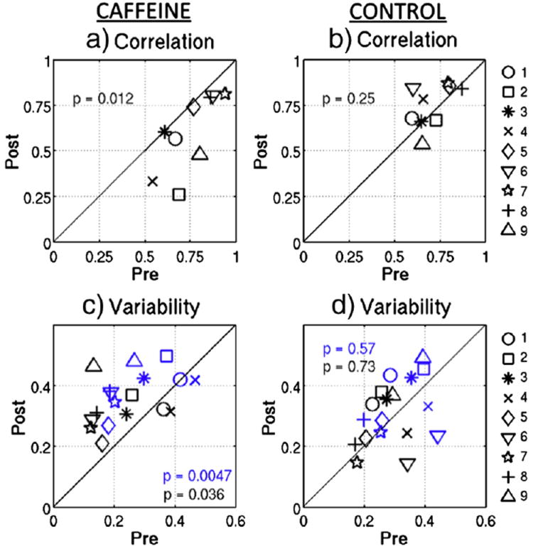
Static measures of inter-hemispheric BOLD correlation are shown for the post-dose versus pre-dose scan sections from a) the caffeine session and b) the control session. Inter-hemispheric BOLD correlation variability measures (standard deviation of sliding window correlation time series) are shown for the post-dose versus pre-dose scan sections during c) the caffeine session and d) the control session. Blue data points were generated using a 20s sliding window and black data points were generated using a 30s window. Solid lines represent equality between the two sections and paired t-test p-values are shown.
Figure 2.
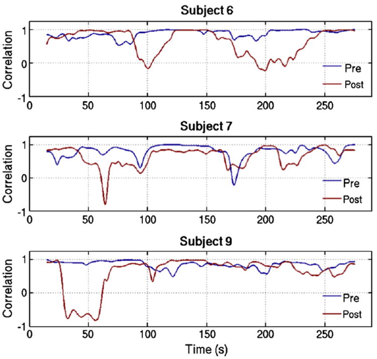
Sliding window correlation time series are shown for 3 representative subjects during the pre-dose (blue line) and post-dose (red line) scan sections, using a representative window length of 30s.
Windowed BOLD signal correlations between the left and right motor cortices are shown as a function of time for three representative subjects in Figure 2, using a representative window length of 30s. While correlation varies with time in both the pre-dose and post-dose scan sections, temporal variability generally appears larger in the caffeinated state. However, extended time periods of strong correlation still exist in the post-dose measures. The scatter plots in Figure 1c and 1d show correlation variability using two representative sliding window lengths of 20s (blue) and 30s (black) for each subject during the caffeine and control sessions, respectively. Caffeine ingestion significantly increased variability for both window lengths (|t(8)| > 2.5, p < 0.04), while the control session data do not display significant changes in variability between scan sections for either window length (|t(8)| < 0.55, p > 0.55). The interaction between imaging section and session measured with a repeated measures two-way ANOVA approaches significance for caffeine-induced variability, with (F(1,8) = 3.9, p = 0.08) for a 20s window and (F(1,8) = 2.88, p = 0.13) for a 30s window. One subject (subject 1) exhibited a greater increase in post-dose correlation variability during the control session as compared to the caffeine session. When this subject is not included, then the ANOVA interaction is significant for both window lengths (F(1,8) > 6, p < 0.04).
To show that the caffeine-induced increase in correlation variability is not specific to a certain window length, caffeine-induced changes in correlation variability are shown as a function of window length in Figure 3, which plots paired t-statistics between the post- and pre-dose scan sections versus window length. T-statistics are shown for both the caffeine session (red circles) and control session (blue circles). In this case a positive t-statistic indicates that variability is larger in the post-dose state, and data points above the top dashed line represent significant (p < 0.05) post-dose increases. Significant caffeine-induced increases in correlation variability are present in the caffeine session for window lengths of 31 seconds and shorter, with a maximum difference occurring for a window length of 18s. Longer windows tend to smooth out correlation variations, making it more difficult to detect the effects of caffeine on correlation variability. In contrast, the control data do not show significant changes in correlation variability between the pre- and post-dose scan sections for any window length. If the regional signal term is not included as a nuisance regressor, we find that correlation variability for the caffeine session data is significantly greater in the caffeinated state for window lengths of 27 seconds and shorter.
Figure 3.
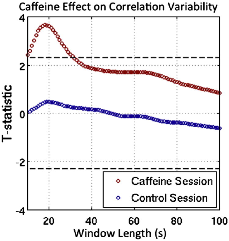
Differences in correlation variability between the post-dose and pre-dose scan sections are plotted versus window length, where red circles are paired t-test statistics for the caffeine session and blue circles are paired t-test statistics for the control session. Values above the top dashed line represent significant (p < 0.05) post-dose increases in variability, and values below the bottom dashed line would represent significantly larger variability in the pre-dose session. Window lengths between 10s and 31s produce significant caffeine-induced changes, with a maximum difference for a window length of 18s. No significant differences in correlation variability were present in the control session data.
BOLD time courses from the left and right motor cortices are shown before and after caffeine ingestion for a representative subject (Subject 9) in the top panel of Figure 4. To visualize temporal variability in cross magnitude and phase, we created time-frequency plots of the windowed cross power spectra, which are shown below the BOLD time courses in Figure 4. These were created by computing the cross power spectrum between the left and right motor cortex BOLD signals for each sliding window period (a representative 30s window was used) and displaying the resulting spectrum as a column in the time-frequency plot. For visualization purposes, we “increased” frequency resolution by zero-padding to 4 times the window length. In the plot, the color scale represents magnitude in units of normalized log-spectrum log2 (MXY [k] / σx σy where σx and σy are the standard deviations computed over the entire length of the two BOLD time courses. Arrows are used to represent phase, with each arrow pointing to a position along the unit circle given by its phase angle. A 90° phase would have an arrow pointing up, a 180° phase would have an arrow pointing to the left, and so on. The frequency axis (y-axis) is restricted to frequencies less than the 0.08 Hz cut-off frequency that was used in the processing of the data. The plots in the bottom row of Figure 4 show sliding window time courses for correlation (black), cosine of the average phase (pink), and average cross power magnitude (light blue).
Figure 4.
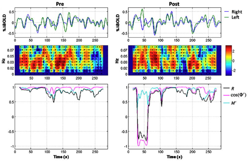
BOLD time courses from the left and right motor cortices are shown for a representative subject in the pre-dose (left plot) and post-dose (right plot) scan sections in the top row. Cross power spectra versus time are shown in the middle row, where the color represents the logarithm to the base 2 of the normalized magnitude and the arrows represent phase differences between the 2 time courses. The bottom row shows correlation (black), cosine of the average cross phase cos( ) (pink), and the average cross magnitude (light blue) versus time.
The power spectra in Figure 4 show that periods of low joint BOLD signal power (blue and green colors) correspond in time with reductions in correlation, shown in the plots below. This relationship is also captured by the time courses (light blue), which appear to track the correlation time courses fairly well, particularly in the pre-dose state. In addition, non-zero phase differences between the two signals (indicated with arrows on the power spectra) also correspond with decreases in the correlation time series shown in the plots below, especially in the post-dose state. The relationship between phase and correlation is shown more clearly in the bottom plots, where is in pink and correlation is in black. From viewing these sliding window time courses, it can be seen that phase offsets between the BOLD time courses approach 180 degrees during the post-dose section, and appear to be responsible for the large drop in correlation. This suggests that larger phase differences, rather than variations in joint signal power, during the post-dose state may be responsible for the caffeine-induced increase in correlation variability.
The scatter plots in the top row of Figure 5 show the R2 values between the sliding window correlation and a) the cosine of the average cross phase , and b) the average cross power magnitude . The plots on the bottom row chart the post-dose versus pre-dose variability (standard deviation of the time series) of and in panels c and d, respectively. In these figures, blue data points were generated using a 20s window and black data points were from a 30s window. It can be seen that temporal variations in phase explain significantly (|t(8)| > 3, p < 0.02) more of the variance in correlation after caffeine ingestion (Fig 5a). Furthermore, similar to the increase in correlation variability, there is a significant (|t(8)| > 3.2, p < 0.02) caffeine-induced increase in phase variability (Fig 5c). On the other hand, explains significantly (|t(8)| > 2.8, p < 0.03) more of the sliding window correlation in the pre-dose section (Fig 5b). However, variability in is greater in the post-dose section (|t(8)| > 2.5, p < 0.04) (Fig 5d). It seems likely that fluctuations in joint signal power produce variations in BOLD correlation during both the pre-dose and post-dose states. However, because phase variations (mean variability of 0.49 and 0.41 for 20s and 30s windows, respectively) are substantially larger in the post-dose state than joint power fluctuations (mean variability of 0.19 and 0.18 for 20s and 30s windows, respectively), the relationship between BOLD correlation and may be partially masked in the post-dose data. Note that the control session data did not show significant differences between scan sections for any of the metrics shown in Figure 5 (|t(8)| < 1.1, p > 0.3).
Figure 5.
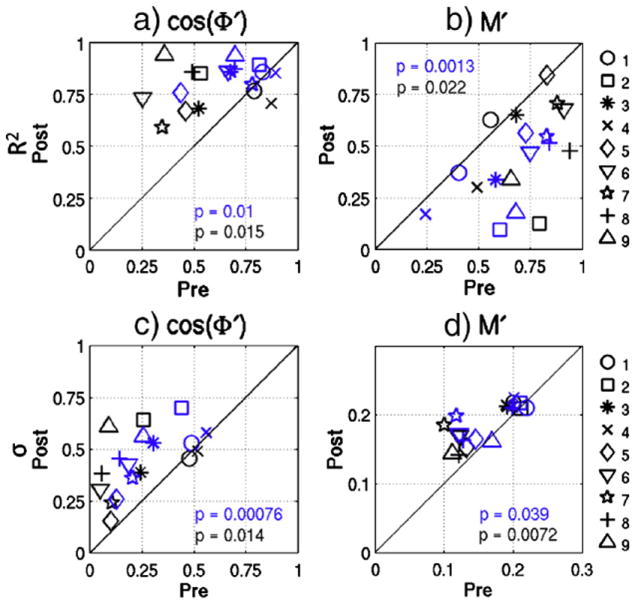
R2 values between sliding window BOLD correlation and a) and b) for the post-dose versus pre-dose scan sections. Variability values (standard deviation of the sliding window time courses) are plotted for c) and d) before and after caffeine ingestion. Blue data points were generated using a 20s sliding window and black data points were generated using a 30s window. The solid line represents equality between the sections, and paired t-test p-values are shown.
Metrics for the temporal variability of the nuisance signals were also examined. There were no significant caffeine-related differences in either the mean variability (p > 0.28 for 20s time window; p > 0.26 for 30s time window) or the standard deviation variability (p > 0.49 for 20s time window; p > 0.26 for 30s time window). These results suggest that the observed caffeine-induced changes in the temporal variability of the correlation are not likely to be due to differences in the stationarity of the nuisance signals. Even if a significant difference had been observed, a straightforward interpretation would have been difficult. This is because the removal of non-stationary regressors can either increase or decrease the stationarity of the resulting correlations. For example, a large sudden movement would cause the motion regressors to be non-stationary, but regressing out its effects could produce a cleaner set of BOLD signals with inter-regional correlations that are more stationary. On the other hand, the removal of a regressor with a large spike that is not reflected in the original data could impose a large transition in the corrected data, leading to greater non-stationarity in the correlations.
Discussion
Caffeine has been previously shown to reduce stationary measures of the correlation between spontaneous BOLD signal fluctuations in the motor cortex (Rack-Gomer et al. 2009). However, because of the complexity of caffeine’s interaction with both the neural and vascular systems, it remains unclear how BOLD signal correlation is disrupted. In this study, we examined temporal variations in correlation before and after a 200mg dose of caffeine to gain more insight into the physiological mechanisms of caffeine’s effect on functional connectivity. We found that correlations between left and right motor cortex BOLD signals showed significantly more temporal variability following a caffeine dose. Furthermore, these variations appear to be driven by phase differences between the signals.
Fluctuations in BOLD correlation, particularly those dependent on phase differences, may reflect the underlying dynamic nature of neural activity coherence. Transient episodes of inter-regional phase-locking of neural activity have been theoretically simulated in models based on the known anatomical connectivity of the primate brain (Honey et al. 2007) and demonstrated in vivo (Varela et al. 2001). In addition, transient periods of strong correlations were found between magnetoencephalography (MEG) power fluctuations within distributed resting-state networks, revealing the presence of nonstationary neuronal dynamics in the human brain (de Pasquale et al. 2010). This temporal variability in neural activity correlation was predominantly seen between hemispheres. While a relationship between BOLD fluctuations and electrical power fluctuations has been shown using simultaneous electroencephalography (EEG) and fMRI (Goldman et al. 2002; Laufs et al. 2003; Moosmann et al. 2003; de Munck et al. 2007; Ritter et al. 2008), BOLD fluctuations have generally produced stronger and more stationary correlations within functional networks than those found with EEG or MEG. It has been hypothesized that the hemodynamic response function (HRF) smoothes out this temporal variability. However, very slow (0.15-0.5 Hz) modulations in local field potential (LFP) power have been shown to exhibit large and variable phase differences between the cat homologues of the DMN and task positive network (TPN) (Popa et al. 2009), which would not be masked by HRF smoothing. Furthermore, previous work has shown variable phase differences between BOLD time courses in the DMN and TPN (Chang and Glover 2010). These variations are also found in the data presented in this study.
Caffeine caused greater variability in the correlation between resting BOLD time courses in the left and right motor cortices. The mode of interhemispheric coordination of spontaneous oscillations in neural activity is not known for certain. One possibility is that homologous activity in the left and right sensorimotor cortex is primarily mediated by the corpus callosum (Johnston et al. 2008). However, it is also possible that the thalamus, which serves as a relay center for both sensory and motor mechanisms (Herrero et al. 2002), coordinates spontaneous activity between the motor cortex hemispheres (MacDonald et al. 1996; Uddin et al. 2008). Previous studies have shown that caffeine stimulates motor activity by counteracting the inhibitory control exerted by adenosine receptors on striatal dopamine transmission, which will ultimately disinhibit thalamo-cortical projection neurons (Fisone et al. 2004; Fontanez and Porter 2006). Caffeine’s direct impact on the pathway between the thalamus and the cortex may increase variability in the coordination of neural activity between these two sites, which could lead to the correlation variability between hemispheres observed in this study.
As caffeine antagonism of adenosine receptors produces both neural and vascular effects, which in turn both influence the BOLD signal, the increased temporal variability in BOLD correlation might also reflect changes in the vasculature that reduce the BOLD signal’s sensitivity to underlying neural activity. This could be accomplished either through caffeine’s inhibition of adenosine-induced dilation of blood vessels (Meno et al. 2005; Pelligrino et al. 2010) or its reduction of the ratio between blood flow changes and oxygen metabolism changes in response to neural activity (Chen and Parrish 2009). If the BOLD signal is less sensitive to underlying neuronal fluctuations, then a larger proportion of noise of non-neural origins could be present in the resting-state BOLD time courses. This decrease in signal to noise ratio could lead to the observed reductions in stationary correlation and increased temporal variability in correlation without an accompanying change in the coherence of spontaneous neural activity. However, it is unlikely that increased physiological noise in the BOLD signal is primarily responsible for the findings presented here. This is because we find extended periods of strong correlation in the post-dose condition that are unlikely to be present if there was an overall decrease in signal-to-noise ratio. Furthermore, preliminary work by our group with MEG measures, which are insensitive to caffeine’s vascular effects, has shown that caffeine also reduces stationary measures of correlation in the motor cortex (Tal et al. 2011). Future work with simultaneous electroencephalographic (EEG) and fMRI measures will be useful in elucidating whether caffeine directly increases phase variability between neural activity in the left and right motor cortices.
In conclusion, we find that correlation between the BOLD signals in the left and right motor cortices varies over time, and that this variability is significantly increased by caffeine. The predominant source of these variations appears to be the non-stationarity of the phase differences between the two signals. These results suggest that caffeine causes greater variability in the underlying coherence of neural activity. As caffeine is a widely consumed stimulant, its effects on functional connectivity should be considered as a potential confound for other restingstate disease and drug studies. Furthermore, future studies assessing changes in functional connectivity caused by other pharmaceutical agents or diseases will benefit from considering not just stationary measures of functional connectivity, but dynamic properties as well.
Acknowledgments
We thank Joanna Perthen and Joy Liau for their assistance with this study. This work was supported in part by a grant from the National Institutes of Health (R01NS051661).
Appendix
Derivation of Cross Power Spectral Representation of the Correlation Coefficient
Let x[n] and y[n] represent average resting-state BOLD time courses from the left and right motor cortex ROIs, respectively, and assume that the means of these time courses have been subtracted. The correlation coefficient between x[n] and y[n], which are both of length N, is defined as
| (A.1) |
By applying Parseval’s Theorem, the above expression can be written in terms of the discrete Fourier Transforms of x[n] and y[n], which are denoted as X[k] and Y[k], respectively. Parseval’s Theorem states that
| (A.2) |
where horizontal bars represent complex conjugation (Oppenheim and Schafer 1989). Since x[n] and y[n] are real-valued signals, and equation A.1 can be written as
| (A.3) |
The frequency indexing in equation A.3 starts at 1 instead of zero because the means have been removed from x[n] and y[n], and hence X[0] = Y[0] = 0. Using the definitions for power spectra and cross power spectra provided in the Methods section, equation A.3 can be written as
| (A.4) |
which is the cross power spectral representation of the correlation coefficient. Note that a 1/fs term, where fs is the sampling rate, is also present in the definitions for power spectra, but this term will divide out in the above expression.
The cross power spectral representation of the correlation coefficient can be decomposed into the product of average cross magnitude and phase components. To show this, we first note that because the signals are real, the cross power spectrum exhibits conjugate symmetry (Oppenheim and Schafer 1989). Then the sum in the numerator of Equation A.4 may be written as
| (A.5) |
where we have assumed that the length N is an even number and made use of the fact that PXY [N /2] is real. For signals with an odd length N, the sum may be written as
| (A.6) |
By substituting equation A.5 into equation A.4 it can be seen that the cross power spectral representation of the correlation coefficient can be decomposed into the product of an “average” cross magnitude component and cross phase component, which we will call and , respectively. Thus, R can be written as
| (A.10) |
where
| (A.11) |
and
| (A.12) |
Footnotes
Publisher's Disclaimer: This is a PDF file of an unedited manuscript that has been accepted for publication. As a service to our customers we are providing this early version of the manuscript. The manuscript will undergo copyediting, typesetting, and review of the resulting proof before it is published in its final citable form. Please note that during the production process errors may be discovered which could affect the content, and all legal disclaimers that apply to the journal pertain.
References
- Birn RM, Smith MA, Jones TB, Bandettini PA. The respiration response function: the temporal dynamics of fMRI signal fluctuations related to changes in respiration. Neuroimage. 2008;40(2):644–54. doi: 10.1016/j.neuroimage.2007.11.059. [DOI] [PMC free article] [PubMed] [Google Scholar]
- Biswal B, Hudetz AG, Yetkin FZ, Haughton VM, Hyde JS. Hypercapnia reversibly suppresses low-frequency fluctuations in the human motor cortex during rest using echo-planar MRI. J Cereb Blood Flow Metab. 1997;17(3):301–8. doi: 10.1097/00004647-199703000-00007. [DOI] [PubMed] [Google Scholar]
- Biswal B, Yetkin FZ, Haughton VM, Hyde JS. Functional connectivity in the motor cortex of resting human brain using echo planar MRI. Magn Reson Med. 1995;34:537–541. doi: 10.1002/mrm.1910340409. [DOI] [PubMed] [Google Scholar]
- Boynton GM, Engel SA, Glover GH, Heeger DJ. Linear systems analysis of functional magnetic resonance imaging in human V1. J Neuroscience. 1996;16:4207–4221. doi: 10.1523/JNEUROSCI.16-13-04207.1996. [DOI] [PMC free article] [PubMed] [Google Scholar]
- Burock MA, Dale AM. Estimation and detection of event-related fMRI signals with temporally correlated noise: a statistically efficient and unbiased approach. Human Brain Mapping. 2000;11:249–260. doi: 10.1002/1097-0193(200012)11:4<249::AID-HBM20>3.0.CO;2-5. [DOI] [PMC free article] [PubMed] [Google Scholar]
- Buxton RB, Uludag K, Dubowitz DJ, Liu TT. Modeling the hemodynamic response to brain activation. Neuroimage. 2004;23(Suppl 1):S220–33. doi: 10.1016/j.neuroimage.2004.07.013. [DOI] [PubMed] [Google Scholar]
- Cameron OG, Modell JG, Hariharan M. Caffeine and human cerebral blood flow: a positron emission tomography study. Life Sci. 1990;47(13):1141–6. doi: 10.1016/0024-3205(90)90174-p. [DOI] [PubMed] [Google Scholar]
- Chang C, Cunningham JP, Glover GH. Influence of heart rate on the BOLD signal: the cardiac response function. Neuroimage. 2009;44(3):857–69. doi: 10.1016/j.neuroimage.2008.09.029. [DOI] [PMC free article] [PubMed] [Google Scholar]
- Chang C, Glover GH. Time-frequency dynamics of resting-state brain connectivity measured with fMRI. Neuroimage. 2010;50(1):81–98. doi: 10.1016/j.neuroimage.2009.12.011. [DOI] [PMC free article] [PubMed] [Google Scholar]
- Chen Y, Parrish TB. Caffeine’s effects on cerebrovascular reactivity and coupling between cerebral blood flow and oxygen metabolism. Neuroimage. 2009;44(3):647–52. doi: 10.1016/j.neuroimage.2008.09.057. [DOI] [PMC free article] [PubMed] [Google Scholar]
- Cordes D, Haughton VM, Arfanakis K, Carew JD, Turski PA, Moritz CH, Quigley MA, Meyerand ME. Frequencies contributing to functional connectivity in the cerebral cortex in “resting-state” data. AJNR Am J Neuroradiol. 2001;22(7):1326–33. [PMC free article] [PubMed] [Google Scholar]
- Cox RW. AFNI-software for analysis and visualization of functional magnetic resonance neuroimages. Comput Biomed Res. 1996;29:162–173. doi: 10.1006/cbmr.1996.0014. [DOI] [PubMed] [Google Scholar]
- de Munck JC, Goncalves SI, Huijboom L, Kuijer JP, Pouwels PJ, Heethaar RM, Lopes da Silva FH. The hemodynamic response of the alpha rhythm: an EEG/fMRI study. Neuroimage. 2007;35(3):1142–51. doi: 10.1016/j.neuroimage.2007.01.022. [DOI] [PubMed] [Google Scholar]
- de Pasquale F, et al. Temporal dynamics of spontaneous MEG activity in brain networks. Proc Natl Acad Sci U S A. 2010;107(13):6040–5. doi: 10.1073/pnas.0913863107. [DOI] [PMC free article] [PubMed] [Google Scholar]
- Diniz PSR, da Silva EAB, Netto SL. Digital Signal Processing: System Analysis and Design. Cambridge University Press; Cambridge: 2002. [Google Scholar]
- Dunwiddie TV, Masino SA. The role and regulation of adenosine in the central nervous system. Annu Rev Neurosci. 2001;24:31–55. doi: 10.1146/annurev.neuro.24.1.31. [DOI] [PubMed] [Google Scholar]
- Fisone G, Borgkvist A, Usiello A. Caffeine as a psychomotor stimulant: mechanism of action. Cell Mol Life Sci. 2004;61(7-8):857–72. doi: 10.1007/s00018-003-3269-3. [DOI] [PMC free article] [PubMed] [Google Scholar]
- Fontanez DE, Porter JT. Adenosine A1 receptors decrease thalamic excitation of inhibitory and excitatory neurons in the barrel cortex. Neuroscience. 2006;137(4):1177–84. doi: 10.1016/j.neuroscience.2005.10.022. [DOI] [PMC free article] [PubMed] [Google Scholar]
- Fox MD, Snyder AZ, Vincent JL, Corbetta M, Van Essen DC, Raichle ME. The human brain is intrinsically organized into dynamic, anticorrelated functional networks. Proc Natl Acad Sci U S A. 2005;102(27):9673–8. doi: 10.1073/pnas.0504136102. [DOI] [PMC free article] [PubMed] [Google Scholar]
- Fredholm BB, Battig K, Holmen J, Nehlig A, Zvartau EE. Actions of caffeine in the brain with special reference to factors that contribute to its widespread use. Pharmacol Rev. 1999;51(1):83–133. [PubMed] [Google Scholar]
- Glover GH, Li TQ, Ress D. Image-based method for retrospective correction of physiological motion effects in fMRI: RETROICOR. Magn Reson Med. 2000;44(1):162–7. doi: 10.1002/1522-2594(200007)44:1<162::aid-mrm23>3.0.co;2-e. [DOI] [PubMed] [Google Scholar]
- Goldman RI, Stern JM, Engel J, Jr, Cohen MS. Simultaneous EEG and fMRI of the alpha rhythm. Neuroreport. 2002;13(18):2487–92. doi: 10.1097/01.wnr.0000047685.08940.d0. [DOI] [PMC free article] [PubMed] [Google Scholar]
- Greicius MD, Krasnow B, Reiss AL, Menon V. Functional connectivity in the resting brain: a network analysis of the default mode hypothesis. Proc Natl Acad Sci U S A. 2003;100(1):253–8. doi: 10.1073/pnas.0135058100. [DOI] [PMC free article] [PubMed] [Google Scholar]
- Greicius MD, Srivastava G, Reiss AL, Menon V. Default-mode network activity distinguishes Alzheimer’s disease from healthy aging: evidence from functional MRI. Proc Natl Acad Sci U S A. 2004;101(13):4637–42. doi: 10.1073/pnas.0308627101. [DOI] [PMC free article] [PubMed] [Google Scholar]
- Hampson M, Driesen NR, Skudlarski P, Gore JC, Constable RT. Brain connectivity related to working memory performance. J Neurosci. 2006;26(51):13338–43. doi: 10.1523/JNEUROSCI.3408-06.2006. [DOI] [PMC free article] [PubMed] [Google Scholar]
- Herrero MT, Barcia C, Navarro JM. Functional anatomy of thalamus and basal ganglia. Childs Nerv Syst. 2002;18(8):386–404. doi: 10.1007/s00381-002-0604-1. [DOI] [PubMed] [Google Scholar]
- Honey CJ, Kotter R, Breakspear M, Sporns O. Network structure of cerebral cortex shapes functional connectivity on multiple time scales. Proc Natl Acad Sci U S A. 2007;104(24):10240–5. doi: 10.1073/pnas.0701519104. [DOI] [PMC free article] [PubMed] [Google Scholar]
- Johnston JM, Vaishnavi SN, Smyth MD, Zhang D, He BJ, Zempel JM, Shimony JS, Snyder AZ, Raichle ME. Loss of resting interhemispheric functional connectivity after complete section of the corpus callosum. J Neurosci. 2008;28(25):6453–8. doi: 10.1523/JNEUROSCI.0573-08.2008. [DOI] [PMC free article] [PubMed] [Google Scholar]
- Kwak Y, Peltier S, Bohnen NI, Muller ML, Dayalu P, Seidler RD. Altered resting state cortico-striatal connectivity in mild to moderate stage Parkinson’s disease. Front Syst Neurosci. 2010;4:143. doi: 10.3389/fnsys.2010.00143. [DOI] [PMC free article] [PubMed] [Google Scholar]
- Laufs H, Kleinschmidt A, Beyerle A, Eger E, Salek-Haddadi A, Preibisch C, Krakow K. EEG-correlated fMRI of human alpha activity. Neuroimage. 2003;19(4):1463–76. doi: 10.1016/s1053-8119(03)00286-6. [DOI] [PubMed] [Google Scholar]
- Liu TT, Frank LR, Wong EC, Buxton RB. Detection power, estimation efficiency, and predictability in event-related fMRI. Neuroimage. 2001;13(4):759–73. doi: 10.1006/nimg.2000.0728. [DOI] [PubMed] [Google Scholar]
- Lowe MJ, Mock BJ, Sorenson JA. Functional connectivity in single and multislice echoplanar imaging using resting-state fluctuations. Neuroimage. 1998;7(2):119–32. doi: 10.1006/nimg.1997.0315. [DOI] [PubMed] [Google Scholar]
- Lowe MJ, Phillips MD, Lurito JT, Mattson D, Dzemidzic M, Mathews VP. Multiple sclerosis: low-frequency temporal blood oxygen level-dependent fluctuations indicate reduced functional connectivity initial results. Radiology. 2002;224(1):184–92. doi: 10.1148/radiol.2241011005. [DOI] [PubMed] [Google Scholar]
- Lui S, Ouyang L, Chen Q, Huang X, Tang H, Chen H, Zhou D, Kemp GJ, Gong Q. Differential interictal activity of the precuneus/posterior cingulate cortex revealed by resting state functional MRI at 3T in generalized vs. Partial seizure. J Magn Reson Imaging. 2008;27(6):1214–20. doi: 10.1002/jmri.21370. [DOI] [PubMed] [Google Scholar]
- MacDonald KD, Brett B, Barth DS. Inter- and intra-hemispheric spatiotemporal organization of spontaneous electrocortical oscillations. J Neurophysiol. 1996;76(1):423–37. doi: 10.1152/jn.1996.76.1.423. [DOI] [PubMed] [Google Scholar]
- Mednick SC, Cai DJ, Kanady J, Drummond SP. Comparing the benefits of caffeine, naps and placebo on verbal, motor and perceptual memory. Behav Brain Res. 2008;193(1):79–86. doi: 10.1016/j.bbr.2008.04.028. [DOI] [PMC free article] [PubMed] [Google Scholar]
- Meno JR, Nguyen TS, Jensen EM, Alexander West G, Groysman L, Kung DK, Ngai AC, Britz GW, Winn HR. Effect of caffeine on cerebral blood flow response to somatosensory stimulation. J Cereb Blood Flow Metab. 2005;25(6):775–84. doi: 10.1038/sj.jcbfm.9600075. [DOI] [PubMed] [Google Scholar]
- Moosmann M, Ritter P, Krastel I, Brink A, Thees S, Blankenburg F, Taskin B, Obrig H, Villringer A. Correlates of alpha rhythm in functional magnetic resonance imaging and near infrared spectroscopy. Neuroimage. 2003;20(1):145–58. doi: 10.1016/s1053-8119(03)00344-6. [DOI] [PubMed] [Google Scholar]
- Mumford JA, Hernandez-Garcia L, Lee GR, Nichols TE. Estimation efficiency and statistical power in arterial spin labeling fMRI. Neuroimage. 2006;33(1):103–14. doi: 10.1016/j.neuroimage.2006.05.040. [DOI] [PMC free article] [PubMed] [Google Scholar]
- Murphy K, Birn RM, Handwerker DA, Jones TB, Bandettini PA. The impact of global signal regression on resting state correlations: are anti-correlated networks introduced? Neuroimage. 2009;44(3):893–905. doi: 10.1016/j.neuroimage.2008.09.036. [DOI] [PMC free article] [PubMed] [Google Scholar]
- Oppenheim AV, Schafer RW. Discrete-Time Signal Processing. Prentice-Hall; Englewood Cliffs, New Jersey: 1989. [Google Scholar]
- Pelligrino DA, Xu HL, Vetri F. Caffeine and the control of cerebral hemodynamics. J Alzheimers Dis. 2010;20(Suppl 1):S51–62. doi: 10.3233/JAD-2010-091261. [DOI] [PMC free article] [PubMed] [Google Scholar]
- Perthen JE, Lansing AE, Liau J, Liu TT, Buxton RB. Caffeine-induced uncoupling of cerebral blood flow and oxygen metabolism: A calibrated BOLD fMRI study. Neuroimage. 2008;40(1):237–47. doi: 10.1016/j.neuroimage.2007.10.049. [DOI] [PMC free article] [PubMed] [Google Scholar]
- Popa D, Popescu AT, Pare D. Contrasting activity profile of two distributed cortical networks as a function of attentional demands. J Neurosci. 2009;29(4):1191–201. doi: 10.1523/JNEUROSCI.4867-08.2009. [DOI] [PMC free article] [PubMed] [Google Scholar]
- Rack-Gomer AL, Liau J, Liu TT. Caffeine reduces resting-state BOLD functional connectivity in the motor cortex. Neuroimage. 2009;46(1):56–63. doi: 10.1016/j.neuroimage.2009.02.001. [DOI] [PMC free article] [PubMed] [Google Scholar]
- Restom K, Behzadi Y, Liu TT. Physiological noise reduction for arterial spin labeling functional MRI. Neuroimage. 2006;31(3):1104–15. doi: 10.1016/j.neuroimage.2006.01.026. [DOI] [PubMed] [Google Scholar]
- Ritter P, Moosmann M, Villringer A. Rolandic alpha and beta EEG rhythms’ strengths are inversely related to fMRI-BOLD signal in primary somatosensory and motor cortex. Hum Brain Mapp. 2008 doi: 10.1002/hbm.20585. [DOI] [PMC free article] [PubMed] [Google Scholar]
- Roth PR. Effective measurements using digital signal analysis. IEEE Spectrum. 1971;8:62–70. [Google Scholar]
- Song M, Zhou Y, Li J, Liu Y, Tian L, Yu C, Jiang T. Brain spontaneous functional connectivity and intelligence. Neuroimage. 2008;41(3):1168–76. doi: 10.1016/j.neuroimage.2008.02.036. [DOI] [PubMed] [Google Scholar]
- Tal O, Wong CW, Olafsson V, Diwakar M, Huang M-X, Liu TT. Caffeine-induced Reductions in Motor Connectivity: A Comparison of fMRI and MEG Measures. Proceedings of the 19th ISMRM, Montreal. 2011:106. [Google Scholar]
- Uddin LQ, et al. Residual functional connectivity in the split-brain revealed with resting-state functional MRI. Neuroreport. 2008;19(7):703–9. doi: 10.1097/WNR.0b013e3282fb8203. [DOI] [PMC free article] [PubMed] [Google Scholar]
- Varela F, Lachaux JP, Rodriguez E, Martinerie J. The brainweb: phase synchronization and large-scale integration. Nat Rev Neurosci. 2001;2(4):229–39. doi: 10.1038/35067550. [DOI] [PubMed] [Google Scholar]
- Voyvodic JT. Activation mapping as a percentage of local excitation: fMRI stability within scans, between scans and across field strengths. Magn Reson Imaging. 2006;24(9):1249–61. doi: 10.1016/j.mri.2006.04.020. [DOI] [PubMed] [Google Scholar]
- Wong EC, Buxton RB, Frank LR. Quantitative imaging of perfusion using a single subtraction (QUIPSS and QUIPSS II) Magn Reson Med. 1998;39(5):702–708. doi: 10.1002/mrm.1910390506. [DOI] [PubMed] [Google Scholar]
- Woolrich MW, Ripley BD, Brady M, Smith SM. Temporal autocorrelation in univariate linear modeling of FMRI data. Neuroimage. 2001;14(6):1370–86. doi: 10.1006/nimg.2001.0931. [DOI] [PubMed] [Google Scholar]