Conformation Types of Ubiquitin [M+8H]⁸⁺ Ions from Water:Methanol Solutions: Evidence for the N and A States in Aqueous Solution

Abstract

Ion mobility and mass spectrometry measurements are used to examine the gas-phase populations of [M+8H]⁸⁺ ubiquitin ions formed upon electrospraying 20 different solutions: from 100:0 to 5:95 water:methanol that are maintained at pH = 2.0. Over this range of solution conditions, mobility distributions for the +8 charge state show substantial variations. Here we develop a model that treats the combined measurements as one data set. By varying the relative abundances of a discrete set of conformation types, it is possible to represent distributions obtained from any solution. For solutions that favor the well-known A-state ubiquitin, it is possible to represent the gas-phase distributions with seven conformation types. Aqueous conditions that favor the native structure require four more structural types to represent the distribution. This analysis provides the first direct evidence for trace amounts of the A state under native conditions. The method of analysis presented here should help illuminate how solution populations evolve into new gas-phase structures as solvent is removed. Evidence for trace quantities of previously unknown states under native solution conditions may provide insight about the relationship of dynamics to protein function as well as misfolding and aggregation phenomena.

Introduction

While it is widely believed that proteins sample a wide range of structures as they fold and denature, characterization of many different forms has not been possible by use of traditional techniques, such as circular dichroism (CD),¹ Raman spectroscopy,² nuclear magnetic resonance (NMR),^3,4 and crystallography.⁵ This is because few conformers can be trapped, isolated and stabilized for time periods that allow experimental determination of their structures.⁶ One system that has attracted considerable attention is ubiquitin, a small, 76-residue cytoplasmic protein.^7,8 NMR data show that the native state (N) exists in aqueous environments from pH ∼ 1.2 to 8.4.⁹ The N state favors tightly packed three-dimensional configurations that incorporate α- and 3₁₀-helices, a five-stranded β-sheet, and seven reverse turns, as illustrated in Figure 1.¹⁰ Dynamics studies show that on the ns to μs timescale, the C-terminal tail of the protein can sample a wide range of geometries.¹¹ This, and other high-frequency motions, results in configurations that are similar to the 46 different crystal structures for ubiquitin bound to different substrates.¹¹ When dissolved in ∼40:60 water: methanol solutions (pH ∼ 2), a new state (A) is stabilized.^{12, 13} Although its tertiary structure has not been determined directly, NMR and CD studies show that A-state ubiquitin retains some secondary structural features of the N state; however, substantial differences are also apparent.^12-17 For example, the N-terminal half of the A state persists as a networked β-sheet (as in the N state); whereas, the C-terminal half of the protein undergoes a methanol-induced transition that leads to a more elongated structure with high α-helical propensity.¹⁴ Figure 1 illustrates this secondary structure for a relatively extended rendering, similar to illustrations published previously.¹⁴ A number of studies suggest that the A state may be a late-stage intermediate along the pathway from unfolded conformations to the native fold.^{13,15,16,18-20} However, this state has never been directly measured from the aqueous native solution environment. At higher methanol compositions (and under other denaturing conditions) there is evidence for poorly defined unfolded structures, referred to collectively as the U state.^13,21,22 Figure 1 also shows a random-like structure that might resemble an unfolded state.

Figure 1.

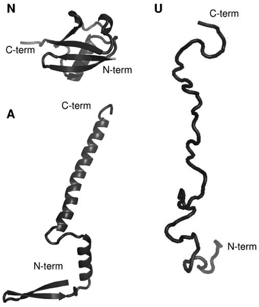
(N) Structure of the native state of ubiquitin.¹⁰ (A) Structural model of the A state of ubiquitin (constructed based on the model proposed in ^{ref. 14}). (U) Structural model of the unfolded state of ubiquitin.

In this paper we use ion mobility spectrometry (IMS) to examine the conformations of ubiquitin [M+8H]⁸⁺ ions produced upon electrospraying 20 water: methanol solutions (from 100:0 to 5:95 water: methanol at pH = 2). Electrospray ionization (ESI)²³ allows populations of states that exist in solution to be transferred to the gas phase where they can be analyzed by a range of mass spectrometry (MS) techniques.^24-29 An issue that is attracting considerable attention is the degree to which in vacuo conformations might resemble distributions of structures that originated from solution.^30-37 One might assume that the process of electrospraying ions would be so disruptive that any resemblance of the ions to solution structures would be lost.³⁰ However, many studies provide evidence that this is not the case and to some extent information about solution states is transferred to the gas-phase ions.^31-37 Recently, Wyttenbach and Bowers provided evidence for the preservation of N-state ubiquitin conformations in the gas phase.³⁸

Below, we focus on characterizing how many different types of gas-phase structures are produced from a range of solution compositions that should favor the N, A, and U states. Our focus is to correlate populations that are present in solution to specific peaks that are observed in the gas-phase measurement. Previous studies show that the IMS distributions obtained from two different solutions are different.³⁹ We investigate [M+8H]⁸⁺ species because upon ESI the percentage of this ion (within the total distribution of different charge states) is nearly constant across all of these solution compositions (an average of 6 ± 2% of the total ion population). This allows us to examine the IMS distributions without complications that arise from variations in ion population due to changes in the charge state distribution.⁴⁰ Additionally, [M+8H]⁸⁺ ions of ubiquitin are interesting because they appear to exist as a wide range of conformations in the gas phase -from compact structures having experimental cross sections that are near the value that is calculated for NMR and crystallographic coordinates of the N state, to extended geometries that must retain very little tertiary structure.⁴¹ Lower ubiquitin charge states (e.g., +7, and to a lesser extent +6) favor compact structures and are the most abundant charge states when electrosprayed from aqueous N-state solution conditions; higher charge states (+10 to +13) adopt elongated conformations because these structures reduce the relatively large repulsive Coulombic interactions.^41,42 ESI favors high charge states (e.g., +10 to +12) when ubiquitin is electrosprayed from non-native (high-methanol) solution conditions. The large range of geometries for the intermediate +8 charge state arises because of a delicate balance of repulsive interactions and attractive folding forces (e.g., hydrogen- and van der Waals-bonding interactions).⁴³ Thus, this charge state becomes a target for understanding the number of isolatable states for a relatively small model system. Below, we show that it is possible to model distributions of ions formed from all solutions by a single set of gas-phase structures. The only difference between the distributions from different solutions is the conformer populations. This model provides new insight about how populations that are present in solution evolve into gas-phase ions during the electrospray process. For example, we were surprised to find that trace amounts of the A state emerge as the +8 charge state upon electrospraying from native solution conditions.

Experimental

IMS-MS methods

IMS measurements,^44-46 instrumentation,^47-57 and theory^44,58-61 are described in detail elsewhere. Only a brief description of the experimental setup as it pertains to the analysis presented below is given here. The instrument consists of an electrospray source, a drift tube and a time-of-flight (TOF) MS detector. The drift tube is 183 cm in length and is filled with ∼3.5 Torr of helium buffer gas (300 K). For the current experiments, protein solutions (ubiquitin – see below) are electrosprayed by a TriVersa NanoMate autosampler (Advion, Ithaca, NY). Ions are accumulated in an hour-glass ion funnel⁵⁷ and periodically released into the drift tube. Ions traverse the drift tube under the influence of a 10 V·cm^-1 uniform electric field over ∼20 to 30 ms. Upon exiting the drift tube, ions are extracted, and analyzed by MS. Flight time distributions are recorded in a nested fashion, enabling the creation of a two-dimensional data set containing drift time (t_D) and mass-to-charge (m/z) information for all ions, as described previously.⁵⁰ It is worthwhile to note that as the ions drift through the buffer gas, diffusion results in a diffuse ion packet. As described previously,⁶² the drift tube incorporates ion funnel regions to focus these ions and improve transmission efficiency. We note that the field from the dc bias across the ion funnel is maintained sufficiently higher than the drift field in order to eliminate peak broadening associated with ion transmission in the ion funnel regions.⁶²

Determination of experimental collision cross sections

It is often useful to plot data on a collision cross section scale. We convert calibrated drift time distributions to cross section distributions by using the following relation:⁴⁴

$$\Omega =\frac{{\left(18\pi \right)}^{1/2}}{16}\frac{ze}{{\left(k_{\text{b}}T\right)}^{1/2}}{\left[\frac{1}{m_{\mathrm{I}}}+\frac{1}{m_{\mathrm{B}}}\right]}^{1/2}\frac{t_{\mathrm{D}}E}{L}\frac{760}{P}\frac{T}{273.2}\frac{1}{N}$$ (1)

Here, ze corresponds to the ion's charge, k_b is Boltzmann's constant, m _I is the mass of the ion, and m_B is the mass of the buffer gas. The variables E and L are the electric field and the drift length, respectively. P and T correspond to the buffer gas pressure and temperature, respectively. N is the neutral number density of the buffer gas at STP. The need to calibrate data sets arises because of the non-linear fields introduced in the ion funnel (overall this results in only small shifts in the drift time). The calibration is performed as described previously using direct measurement of the drift time through a drift region that does not contain ion funnels.⁶³

Calculation of theoretical cross sections for the structures shown in Figure 1

Atomic coordinates for the N state were taken from Protein Data Bank (pdb file 1UBQ).¹⁰ Coordinates for the ubiquitin A state were obtained by constructing the appropriate secondary structure using the Insight II molecular modeling software (Accelrys Inc., San Diego, CA). This rendering is similar to a model depicted previously.¹⁴ The U-state coordinates correspond to a structure that has very little secondary or tertiary structure. We intended this conformation to be extended and constructed it by carrying out molecular dynamics simulations for the [M+13H]¹³⁺ ion. The high Coulomb energy associated with this charge state forces ubiquitin to adopt highly unfolded geometries. Cross sections are calculated using the projection approximation,^64-66 exact hard sphere scattering,⁵⁹ and trajectory methods⁶⁰ developed by M. F. Jarrold's group and available as the MOBCAL program. All cross sections reported here were obtained by the trajectory method.

Sample preparation

Lyophilized ubiquitin from bovine erythrocytes (≥98%, Sigma-Aldrich Co, St. Louis, MO) was used without further purification. Protein was dissolved in water: methanol mixtures to a final concentration of ∼1·mg·mL^-1. Twenty water and methanol solution compositions, ranging from 100:0 to 5:95 water: methanol (V:V, where the fraction of methanol was increased by 5% for each solution), were prepared. Formic acid was added to each solution to adjust the pH to 2.0 (direct measurement). Our previous studies have employed water: acetonitrile solutions.⁴¹ However, because the A state has been characterized in water: methanol solutions by CD and NMR,^12,14 we have selected this solvent system for the present studies.

Data analysis

The cross section distributions are modeled with a set of Gaussian functions by the Peak Analyzer tool in OriginPro 8.5.0 software (OriginLab Corporation, Northampton, MA). Here the distribution of a single gas-phase conformation type is represented by a Gaussian function. The minimum number of gas-phase conformation types comprising the experimental cross section distribution is estimated by the minimum number of Gaussian functions necessary to represent the distributions arising from the analysis of the multiple protein solutions. Peak centers and widths have been varied iteratively to determine the best settings for modeling all 20 distributions of the ubiquitin [M+8H]⁸⁺ ions; once the peak centers and widths have been established, only the peak heights are varied between data sets obtained under different solvent conditions. The residual sum of squares is calculated and used as a measure of the quality of the model. We note that peak fitting techniques have been used previously to determine the composition of ion drift time distributions providing an indication of the numbers and types of gas-phase conformations that are produced upon ionization.^67-69 The model described here is unique in that the same set of Gaussian functions (peak centers and peak widths) representing specific conformations are applied to all drift time distributions (i.e., those obtained upon electrospraying different solvent compositions). This allows the determination of conformation type abundance within each sample comprised of different solution compositions.

We also compare our experimental data to distributions that are calculated for transport of a pulse of ions corresponding to a single structure using the conditions of our drift tube. This distribution is calculated from equation 2,⁴⁴

$$F\left(t\right)=\int \text{d}{t}_{\text{p}}P\left(t_{\text{p}}\right)\frac{C\left[v_{\text{D}}+L/\left(t-t_{\text{p}}\right)\right]}{{\left(\mathit{\text{D}}T\right)}^{1/2}}\times \left\{1-exp\left[\frac{-r_0^2}{4D\left(t-t_{\text{p}}\right)}\right]\right\}exp\left\{\frac{-{\left[L-v_D\left(t-t_{\text{p}}\right)\right]}^2}{4D\left(t-t_{\text{p}}\right)}\right\}$$ (2)

where dt_pP(t_p) is the distribution function of the packet of ions entering the drift tube, v_D is the drift velocity, C is a constant, r₀ is the radius of the drift tube entrance aperture, and D is the diffusion constant. The original distribution function is based on the ion pulse width (150 μs) used in the experiment. Under low-field conditions, D = v_Dk_BT/(zeE).

Results and discussion

Overview of collision cross section distributions for [M+8H]⁸⁺ ubiquitin ions from different solutions

Figure 2 shows representative cross section distributions for [M+8H]⁸⁺ ions of ubiquitin produced from six of the twenty water: methanol solutions. (The mass spectra for ions electrosprayed from these six solutions are provided as supplementary information and the cross section distributions for [M+8H]⁸⁺ ubiquitin ions generated from the twenty water: methanol solutions are also provided in the supplementary information section.) We note that solution concentrations that are intermediate between those shown in Figure 2 appear only slightly different from one another, such that differences that are observed in Figure 2 appear gradually as the solution composition is varied. For reference the calculated cross sections for the N, A, and U structures (Figure 1) are 1090, 1640, and 1900 Ų, respectively. When ions are formed from the 100:0 solution, we observe a sharp peak in the cross section distribution at 1020 Ų (corresponding to relatively compact conformers that are ∼6% smaller than the calculated value for the N state) and a broad distribution extending from ∼1040 to ∼1620 Ų. Two very small sharp peaks at relatively large cross section values of 1650 and 1680 Ų are also observed. These ions have cross sections that are ∼12-13% smaller than values calculated for the extended U-state coordinates; the peaks are within ∼1-2% of the A-state structure (Figure 1).

Figure 2.

Collision cross section (ccs) distributions for [M+8H]⁸⁺ ubiquitin ions from six different water:methanol solutions. The plots have been obtained from nested t_D(m/z) data sets where all m/z bins over a narrow range (corresponding to [M+8H]⁸⁺ ubiquitin ions) have been integrated for each t_D bin. Solution compositions (water:methanol) are provided as labels for each of the distributions. The data sets have been normalized by using the integrated peak intensity. Dashed lines are drawn to indicate the calculated ccs for the N, A, and U state model structures shown in Figure 1.

As the methanol concentration is increased, substantial changes in the cross section distributions are observed. The distribution obtained upon ESI of the 85:15 solution shows that the relative abundance of the sharp peak at 1020 Ų decreases and the broad feature appears to shift to lower cross sections as well as change in relative intensity. When the solution composition reaches 70:30 the peak at 1020 Ų has all but disappeared. This solution favors two broad features centered at ∼1150 and 1450 Ų and the two sharp peaks at 1650 Ų and 1680 Ų. As the methanol content is increased further, slight shifts in the positions of the broad features are apparent.

Overall, at least some of the changes observed in our data set appear to be consistent with changes in structure known from solution studies. For example, under aqueous conditions we favor the relatively compact 1020 Ų peak. This peak disappears with increased methanol and new states are favored. Other peaks appear to be associated with structures that are favored from high methanol solutions. For example, the sharp features at 1650 and 1680 Ų are clearly apparent at 70:30 and higher methanol content. Additionally two broad features are resolved as the fraction of water is decreased. These peaks appear to arise from the A- and U-state solution populations. We speculate that the sharp features at 1020, 1650 and 1680 Ų in the datasets correspond to conformations that are very similar to the solution structures determined for the N state (first feature) and the A state (latter two features).

Representing IMS features as Gaussian functions

The complete data set described above for the 20 solutions shows that there are gradual changes in the cross section distributions with variations in methanol percentage. This suggests that small changes in the populations of a fixed number of conformer types may account for the observed solvent-dependent cross section distributions. Here, we develop a model that allows us to describe the distributions obtained from all solutions. We begin by assuming that the measured distribution intensity (I) at each cross section (for all solutions) can be represented by a set of Gaussians, each having the form,

$$I=\frac{A}{\sigma \sqrt{2\pi }}{e}^{-\frac{{\left(\Omega -{\Omega }_{\mathit{0}}\right)}^2}{2{\sigma }^2}}$$ (3)

where Ω₀ represents the center of the distribution of each conformation type, σ corresponds to the width of the distribution of states that are populated within each type and A corresponds to the population of each conformation type. Initially, we do not know: 1) the number of conformer types; 2) the mean cross section associated with each type; or, 3) the width of the distribution associated with each conformer type. Progress in refining these variables for the entire data set is made by modeling the sharp peaks that are observed for specific solutions. For example, at the 100:0 extreme, we determine the position and width of the sharp peak Ω = 1020 ± 6 Ų. Comparison with the transport equation (Equation 2) for ions drifting through our instrument indicates that this peak shape is very near what is anticipated for one or two conformations with defined cross sections. Similarly the 5:95 solution allows us to define two Gaussians representing conformer types with Ω = 1650 ± 11 and Ω = 1680 ± 6 Ų. The latter peak is also similar to that expected from Equation 2 for a distribution containing only a single structure. Other features in the data are represented by conformer types that require broader distributions (in some cases ∼15 different transport limited structures would be needed to represent these broad features). Once specific features are determined, they can be subtracted from the data and an iterative process is used to define the number of states required to represent the distributions across all solution compositions.

Figure 3 illustrates this process in more detail. If we include 2 additional broad peaks with positions and distribution widths that are obtained by examining data recorded from the 70:30 to 30:70 solutions, we find that many of the subtle features for other solution compositions are not described accurately. As an example consider the ∼1050 to 1550 Ų region (Figure 3A). Five Gaussian conformer types allow us to pick up the sharp features in all solutions; additionally the broad features in the 70:30 to 30:70 solutions are reasonably well represented. However, the 100:0 to 75:25 solutions are not well represented as a main portion of the ion population centered at ∼1350 Ų is missed.

Figure 3.

Gaussian models of collision cross section (ccs) distributions of [M+8H]⁸⁺ ubiquitin ions electrosprayed from six different water:methanol solutions. Solution compositions (water:methanol) are provided as labels for each of the distributions. Panels A, B, and C have utilized 5, 8, and 11 Gaussian functions respectively, to model the data sets. The experimental data (normalized) are plotted as solid circles, the Gaussian functions are plotted as black solid lines and the sum of the Gaussian functions is plotted as a red dashed line. In Panel C, conformer types that are assigned to the N, A and U states of ubiquitin are plotted in blue, green and pink, respectively (see text for more details).

Figure 3 also shows the results obtained when 5 additional distributions are included (such that there are 8 total Gaussian conformer types in our analysis). The model is much better (Figure 3B). However, the regions between 1050 to 1100 Ų are not well represented from more aqueous solutions. The region 1570 to 1630 Ų is poorly captured for data obtained from high methanol solutions. When 8 additional Gaussian distributions are included (i.e., a total of 11 structural types), the model appears to capture all of the main features that are observed for every solution condition. Figure 3C shows this for the 11 chosen distributions.

More progress in assessing how many conformer types are required to best model all the data can be obtained by calculating the average residual sums of squares for models of all 20 distributions over the range of different numbers of Gaussians that are employed. The result of this analysis is shown in Figure 4. This plot shows that substantial improvements in the ability to represent the complete data set are found as the number of Gaussians is increased to ∼10 or 11. Beyond this value, the improvement for each added Gaussian adds little to the accuracy of representing the entire data set. Table 1 lists a description of each Gaussian and its contribution to the distribution recorded for all 20 solutions that we obtain by assuming 11 conformer types are present.

Figure 4.

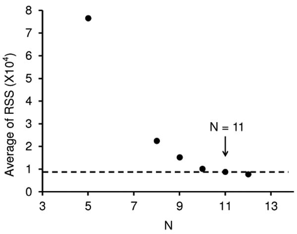
Plot of the average residual sums of squares (RSS) obtained from the Gaussian models of the 20 distributions against the number of Gaussian functions (N) employed.

Table 1. Relative intensity for the 11 conformation types of ubiquitin [M+8H]⁸⁺ ions (distributions represented by Gaussian functions) at different solution compositions.

%MeOH	Relative Intensity for Conformation Typesa											Sumc
	Nb1	N2	N3	Ub	N4	N5	N6	Ab1	A2	A3	A4	N	A	U
	1020 (6)d	1040 (25)	1120 (41)	1160 (60)	1210 (34)	1290 (42)	1360 (47)	1450 (49)	1570 (28)	1650 (11)	1680 (6)
0	0.039	0.056	0.184	0.000	0.147	0.178	0.272	0.112	0.007	0.002	0.003	0.876	0.124	0.000
5	0.054	0.112	0.179	0.000	0.124	0.198	0.223	0.100	0.007	0.002	0.002	0.889	0.111	0.000
10	0.028	0.048	0.174	0.000	0.165	0.206	0.220	0.144	0.009	0.003	0.004	0.840	0.160	0.000
15	0.024	0.042	0.214	0.055	0.189	0.167	0.108	0.180	0.011	0.005	0.006	0.744	0.201	0.055
20	0.035	0.055	0.206	0.180	0.137	0.083	0.071	0.204	0.014	0.006	0.009	0.587	0.233	0.180
25	0.017	0.024	0.155	0.265	0.036	0.031	0.067	0.346	0.025	0.015	0.020	0.330	0.405	0.265
30	0.002	0.000	0.084	0.199	0.024	0.019	0.050	0.517	0.042	0.026	0.037	0.180	0.621	0.199
35	0.000	0.000	0.065	0.210	0.013	0.029	0.020	0.548	0.046	0.028	0.042	0.127	0.663	0.210
40	0.000	0.000	0.060	0.246	0.000	0.038	0.000	0.539	0.043	0.031	0.043	0.098	0.656	0.246
45	0.000	0.000	0.043	0.233	0.000	0.031	0.000	0.582	0.046	0.026	0.039	0.075	0.693	0.233
50	0.000	0.000	0.050	0.259	0.000	0.032	0.000	0.541	0.045	0.029	0.044	0.082	0.659	0.259
55	0.000	0.000	0.055	0.241	0.000	0.039	0.000	0.549	0.046	0.027	0.043	0.094	0.665	0.241
60	0.000	0.000	0.050	0.237	0.000	0.043	0.000	0.555	0.046	0.028	0.041	0.093	0.669	0.237
65	0.000	0.000	0.040	0.302	0.000	0.133	0.000	0.442	0.033	0.021	0.030	0.173	0.525	0.302
70	0.000	0.000	0.036	0.399	0.000	0.087	0.000	0.386	0.037	0.022	0.033	0.123	0.478	0.399
75	0.000	0.000	0.057	0.256	0.000	0.040	0.000	0.533	0.043	0.028	0.043	0.097	0.647	0.256
80	0.000	0.000	0.070	0.266	0.000	0.046	0.000	0.501	0.045	0.030	0.042	0.116	0.618	0.266
85	0.000	0.000	0.072	0.385	0.000	0.047	0.000	0.398	0.041	0.023	0.035	0.120	0.496	0.385
90	0.000	0.000	0.034	0.418	0.000	0.090	0.000	0.364	0.039	0.022	0.032	0.125	0.458	0.418
95	0.000	0.000	0.046	0.446	0.000	0.050	0.000	0.362	0.040	0.021	0.034	0.096	0.458	0.446

^aThe reported intensities are obtained by dividing the area of each Gaussian distribution by the total area for each solution.

^bThe solution phase state (N, A, or U) assigned to the respective gas-phase conformation type.

^cThe sum of relative intensities of different gas-phase conformation types.

^dValues of the center of the 11 Gaussian distributions and the standard deviation of the distributions as represented by Ω₀ (σ) where Ω₀ has units of Ų.

On the relationship of the N, A and U solution states to gas-phase conformer types

It is interesting to consider the analytical implications of the analysis presented above. One way to do this is to plot the populations that are obtained upon modeling all solutions for the specific gas-phase conformer types that were found in the analysis above. We use the 11 conformer type model that is summarized in Table 1. There is little ambiguity about the Ω = 1020 ± 6, Ω = 1650 ± 11 and Ω = 1680 ± 6 Ų distributions, since the sharp nature of these peaks (and their positions at extreme points in the distributions) allows them to be followed visually. Figure 5A shows that the Ω = 1020 Ų conformation type is most abundant from aqueous solutions. As the methanol content increases, the relative abundance of the gas-phase conformer type decreases, until it is no longer observable within our detection limits (for the 65:35 solution). This behavior indicates that this gas-phase conformer type arises from N states that were present in solution. We note that this is the most compact state that is observed for the +8 charge state. The sharp nature of the peak suggests that it was well defined in solution and it emerges as well defined structure in the gas phase. The cross section is slightly smaller than the 1090 Ų value calculated for the N structure in Figure 1. Thus, the ion must have contracted slightly upon desolvation.

Figure 5.

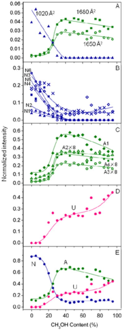
Plots of peak intensity as a function of solvent methanol percentage for different gas-phase conformation types. (A) shows intensities for the three sharp conformer types having Ω = 1020 ± 6 ( ), Ω = 1650 ± 11 ( ) and Ω = 1680 ± 6 Ų ( ). The most compact feature has been assigned to the N state and the more elongated features have been assigned to the A state. (B), (C) and (D) show intensities for the gas-phase conformers that are assigned to the solution states of ubiquitin, N, A, and U, respectively. The labels N1-N6, A1-A4, and U correspond to the assignments in Table 1. N1:1020 ± 6 Ų ( ), N2: 1040 ± 25 Ų ( ), N3: 1120 ± 41 Ų ( ), N4: 1210 ± 34 Ų ( ), N5: 1290 ± 42 Ų ( ),N6: 1360 ± 47 Ų ( ); A1: 1450 ± 49 Ų ( ), A2: 1570 ± 28 Ų ( ), A3: 1650 ± 11 Ų ( ), A4: 1680 ± 6 Ų ( ); U: 1160 ± 60 Ų ( ). Intensity multiplication factors are listed for specific conformer types. (E) shows the sum of the intensities for different gas-phase conformation types that are assigned to the N, A and U states of ubiquitin. Conformer types that are assigned to the N, A and U states of ubiquitin are plotted in blue, green and pink, respectively.

The plot of the percentage of the Ω = 1650 ± 11 and Ω = 1680 ± 6 Ų peaks shows a different profile (Figure 5A). These peaks are most abundant when the gas-phase conformer types are produced from 30:70 to 70:30 solutions. As the fraction of water in these solutions increases the abundance of these features drops dramatically. This behavior is consistent with what we would anticipate for the A structure from solution. It is also remarkable that both cross sections are similar to the 1640 Ų value that we calculated for the A-state coordinates (Figure 1). This suggests that an A state of this type may be transferred into the gas phase while retaining much of its solution structure. We note that there are many other gas-phase configurations that would have this cross section; however, the cross section value combined with the narrow peak width suggest that a direct correlation may exist.

It is interesting that both of these sharp peaks appear to arise from the solution A state. This could be interpreted several ways. It may be that there must be more than one A state in solution, and that we have resolved each of these states upon desolvation. Another interpretation is that the A state from solution splits into two peaks because of differences that arise during the ESI process. For example, slight differences in the locations of the charge sites may lead to differences in the structures of the gas-phase ions. With either interpretation, we were surprised to see the small peaks associated with the A states in the distribution of the 100:0 solution. This interpretation provides the first direct evidence that the A state is present in equilibrium with the N state, even in the 100:0 N-state solution. We also note that another explanation for the data is that the A state is formed during the ESI process. Previous studies have shown that significant ion activation is required to induce structural transformations of compact ubiquitin ions to form more elongated conformers.⁶³ Mobility selections of features corresponding to different conformations within the [M+8H]⁸⁺ distribution also do not provide evidence for structural transformations. This suggests that the A state conformation type observed under native conditions arises in solution rather than as a result of the ESI process. However, we cannot entirely rule out the latter explanation. That such a state was not detected by more conventional methods is consistent with the relatively low abundance of this peak. The +8 charge state comprises 6 ± 2% of the charge state distribution, and these two sharp features comprise only ∼0.5% of the cross section distribution. This reveals another aspect of this analysis, showing that under favorable conditions this type of analysis can detect a very small fraction of ions emerging from solution; in this case, only 0.03% of the ions exist as the Ω = 1650 ± 11 and Ω = 1680 ± 6 Ų peaks. Here, the analysis is very sensitive because no other ions are found at such high cross sections (without the unfolding of [M+8H]⁸⁺ ubiquitin ions by collisional activation).^39,41

While we are sensitive to very low abundance species (i.e., ≥ 0.03%) this value may not represent the actual percentage of A state in the native solution. By making similar plots for all 11 Gaussian representations of conformer types, we can begin to assess which other features show abundance profiles that are similar in appearance to those obtained for N and A peaks. If we plot the Ω = 1040 ± 25, Ω = 1120 ± 41, Ω = 1210 ± 34, Ω = 1290 ± 42, and Ω = 1360 ± 47 Ų peaks, we find that these decay as is expected for the N state (Figure 5B). This is fascinating behavior. In these cases, the cross sections and peak widths are different than what is expected from the single structure of Figure 1, which depicts a very static representation of the N-state structure. We cannot resist noting that one interpretation that is consistent with these data is that there may be many types of structures that are present in solution (as observed on ns to μs timescales by NMR).¹¹ In this interpretation, slight differences in well- folded conformer types that exist in solution may be amplified as ions emerge from the solution. Another, interesting interpretation is that a relatively well-defined set of structures from solution is perturbed by the ESI process and that these comprise the observed gas-phase distribution of structures -this interpretation is similar to analyses that we have done previously, which show that ubiquitin may unfold when stored in a trap or injected at high energies into a drift tube.^41,70 We note that Freitas' and Marshall's data showed evidence for two hydrogen/deuterium exchange rates for [M+8H]⁸⁺ ubiquitin ions when trapped for as long as an hour.⁷¹ Thus, from either interpretation provided above, once these ions are dehydrated and in the gas phase it does not appear that they are interconverting as if they are in equilibrium. We also note that the mobility distributions of a number of features that have been mobility selected from the original ion distribution using a technique described previously⁷² show no evidence for structural transformations. Figure 5C shows a plot of all Gaussian type ions that exhibit A-state behavior. The interpretations that were given for the multiple N-state ions can be extended to the A state.

Figure 5D shows the singular gas-phase conformer type (Ω = 1160 ± 60 Ų) that appears to display neither N- nor A-type behavior as the solution composition is varied. We suspect that this type of profile may correspond to what has been deemed U-state ubiquitin.^13,21,22 It is interesting that the cross section is much smaller than the calculated value of 1900 Ų for the U-type structure from Figure 1. We anticipate that unfolded structures that emerge from solution might collapse as solvent is removed. It is also interesting that this peak is broad. This would be consistent with a large distribution of different unfolded structures emerging from solution (or the formation of new states in the gas phase).

Finally, once the solution state is defined from these profiles, it is possible to estimate the fraction of N, A, and U states that contribute to the +8 charge state. The sum of populations for Gaussians that show similar changes with variations in solution is shown in Figure 5E. This plot illustrates that the N state dominates for aqueous solutions, and only the N and A states contribute to the distribution of 100:0 to 90:10 solutions. The methanol-induced transition leads to a large abundance of A-state ubiquitin at a solution composition of ∼75:25 and this state dominates the contribution to the [M+8H]⁸⁺ distribution from there forward. N-state contributions to the [M+8H]⁸⁺ distribution are minimized to ∼10% of the distribution when methanol comprises more than 40% of the solution.

Summary and Conclusions

The collision cross section distributions of [M+8H]⁸⁺ ubiquitin ions obtained by electrospraying different water: methanol solutions (pH maintained at 2.0 with formic acid) have been reported. These distributions change gradually with increased percentage of methanol in the solvent. A new method that employs Gaussian functions to model the data has been used to determine the minimum number of gas-phase conformation types formed upon electrospraying the 20 different solutions. The minimum number of Gaussian distributions required to represent the data set is determined to be ∼11. Examination of the intensities of the conformation types as a function of solution composition suggests that it is possible to correlate the N, A, and U solution structures to the gas-phase conformer types that are observed upon dehydration.

This analysis provides the first direct evidence that the A state exists in trace amounts, even in aqueous solutions that favor the native protein. The sigmoidal shapes of the methanol-induced changes in relative populations are a reflection of the cooperative nature of the transitions between these states. Thus, in aqueous solutions, the N and A states exist in an equilibrium that strongly favors the N state. The ability to detect small non-native populations from native solution may provide new insight into the important roles of protein dynamics in establishing function.^73-76 Especially relevant, may be the contribution of previously unknown populations to misfolding and aggregation phenomena.^77,78

References

- 1.Hoffmann A, Kane A, Nettels D, Hertzog DE, Baumgärtel P, Lengefeld J, Reichardt G, Horsley DA, Seckler R, Bakajin O, Schuler B. Proc Natl Acad Sci USA. 2007;104:105–110. doi: 10.1073/pnas.0604353104. [DOI] [PMC free article] [PubMed] [Google Scholar]
- 2.Balakrishnan G, Weeks CL, Ibrahim M, Soldatova AV, Spiro TG. Curr Opin Struct Biol. 2008;18:623–629. doi: 10.1016/j.sbi.2008.06.001. [DOI] [PMC free article] [PubMed] [Google Scholar]
- 3.Dyson HJ, Wright PE. Chem Rev. 2004;104:3607–3622. doi: 10.1021/cr030403s. [DOI] [PubMed] [Google Scholar]
- 4.Korzhnev DM, Religa TL, Banachewicz W, Fersht AR, Kay LE. Science. 2010;329:1312–1316. doi: 10.1126/science.1191723. [DOI] [PubMed] [Google Scholar]
- 5.Radford SE, Bartlett AI. Nat Struct Mol Biol. 2009;16:582–588. doi: 10.1038/nsmb.1592. [DOI] [PubMed] [Google Scholar]
- 6.Englander SW, Mayne L. Annu Rev Biophys Biomol Struct. 1992;21:243–265. doi: 10.1146/annurev.bb.21.060192.001331. [DOI] [PubMed] [Google Scholar]
- 7.Goldstein G, Scheid M, Hammerling U, Boyse EA, Schlesinger DH, Niall HD. Proc Natl Acad Sci USA. 1975;72:11–15. doi: 10.1073/pnas.72.1.11. [DOI] [PMC free article] [PubMed] [Google Scholar]
- 8.Rechsteiner M. Ubiquitin. Plenum Press; New York: 1988. [Google Scholar]
- 9.Lenkinski RE, Chen DM, Glickson JD, Goldstein G. Biochim Biophys Acta. 1977;494:126–130. doi: 10.1016/0005-2795(77)90140-4. [DOI] [PubMed] [Google Scholar]
- 10.Vijay-Kumar S, Bugg CE, Cook WJ. J Mol Biol. 1987;194:531–544. doi: 10.1016/0022-2836(87)90679-6. [DOI] [PubMed] [Google Scholar]
- 11.Lange OF, Lakomek N–A, Farès C, Schröder GF, Walter KFA, Becker S, Meiler J, Grubmüller H, Griesinger C, de Groot BL. Science. 2008;320:1471–1475. doi: 10.1126/science.1157092. [DOI] [PubMed] [Google Scholar]
- 12.Wilkinson KD, Mayer AN. Arch Biochem Biophys. 1986;250:390–399. doi: 10.1016/0003-9861(86)90741-1. [DOI] [PubMed] [Google Scholar]
- 13.Harding MM, Williams DH, Woolfson DN. Biochemistry. 1991;30:3120–3128. doi: 10.1021/bi00226a020. [DOI] [PubMed] [Google Scholar]
- 14.Brutscher B, Brüschweiler R, Ernst RR. Biochemistry. 1997;36:13043–13053. doi: 10.1021/bi971538t. [DOI] [PubMed] [Google Scholar]
- 15.Stockman BJ, Euvrard A, Scahill TA. J Biomol NMR. 1993;3:285–296. doi: 10.1007/BF00212515. [DOI] [PubMed] [Google Scholar]
- 16.Cordier F, Grzesiek S. Biochemistry. 2004;43:11295–11301. doi: 10.1021/bi049314f. [DOI] [PubMed] [Google Scholar]
- 17.Kony DB, Hünenberger PH, van Gunsteren WF. Protein Sci. 2007;16:1101–1118. doi: 10.1110/ps.062323407. [DOI] [PMC free article] [PubMed] [Google Scholar]
- 18.Sorenson JM, Head-Gordon T. Proteins Struct Funct Genet. 2002;46:368–379. [PubMed] [Google Scholar]
- 19.Zhang J, Qin M, Wang W. Proteins Struct Funct Bioinf. 2005;59:565–579. doi: 10.1002/prot.20430. [DOI] [PubMed] [Google Scholar]
- 20.Jackson SE. Org Biomol Chem. 2006;4:1845–1853. doi: 10.1039/b600829c. [DOI] [PubMed] [Google Scholar]
- 21.Jourdan M, Searle MS. Biochemistry. 2001;40:10317–10325. doi: 10.1021/bi010767j. [DOI] [PubMed] [Google Scholar]
- 22.Mohimen A, Dobo A, Hoerner JK, Kaltashov IA. Anal Chem. 2003;75:4139–4147. doi: 10.1021/ac034095+. [DOI] [PubMed] [Google Scholar]
- 23.Fen JB, Mann M, Meng CK, Wong SF, Whitehouse CM. Science. 1989;246:64–71. doi: 10.1126/science.2675315. [DOI] [PubMed] [Google Scholar]
- 24.Johnson RS, Martin SA, Biemann K. Int J Mass Spectrom Ion Processes. 1988;86:137–154. [Google Scholar]
- 25.Loo JA, Edmonds CG, Smith RD. Science. 1990;248:201–204. doi: 10.1126/science.2326633. [DOI] [PubMed] [Google Scholar]
- 26.Covey T, Douglas DJ. J Am Soc Mass Spectrom. 1993;4:616–623. doi: 10.1016/1044-0305(93)85025-S. [DOI] [PubMed] [Google Scholar]
- 27.Suckau D, Shi Y, Beu SC, Senko MW, Quinn JP, Wampler FM, McLafferty FW. Proc Natl Acad Sci USA. 1993;90:790–793. doi: 10.1073/pnas.90.3.790. [DOI] [PMC free article] [PubMed] [Google Scholar]
- 28.Syka JEP, Coon JJ, Schroeder MJ, Shabanowitz J, Hunt DF. Proc Natl Acad Sci USA. 2004;101:9528–9533. doi: 10.1073/pnas.0402700101. [DOI] [PMC free article] [PubMed] [Google Scholar]
- 29.Pan Y, Brown L, Konermann L. Int J Mass Spectrom. 2011;302:3–11. [Google Scholar]
- 30.Wolynes PG. Proc Natl Acad Sci USA. 1995;92:2426–2427. doi: 10.1073/pnas.92.7.2426. [DOI] [PMC free article] [PubMed] [Google Scholar]
- 31.Baumketner A, Bernstein SL, Wyttenbach T, Bitan G, Teplow DB, Bowers MT, Shea JE. Protein Sci. 2006;15:420–428. doi: 10.1110/ps.051762406. [DOI] [PMC free article] [PubMed] [Google Scholar]
- 32.Pierson NA, Chen L, Valentine SJ, Russell DH, Clemmer DE. J Am Chem Soc. 2011;133:13810–13813. doi: 10.1021/ja203895j. [DOI] [PMC free article] [PubMed] [Google Scholar]
- 33.Ruotolo BT, Robinson CV. Curr Opin Chem Biol. 2006;10:402–408. doi: 10.1016/j.cbpa.2006.08.020. [DOI] [PubMed] [Google Scholar]
- 34.Patriksson A, Marklund E, van der Spoel D. Biochemistry. 2007;46:933–945. doi: 10.1021/bi061182y. [DOI] [PubMed] [Google Scholar]
- 35.Ganem B, Li YT, Henion JD. Tetrahedron Lett. 1993;34:1445–1448. [Google Scholar]
- 36.Goodlett DR, Camp DG, Hardin CC, Corregan M, Smith RD. Biol Mass Spectrom. 1993;22:181–183. doi: 10.1002/bms.1200220307. [DOI] [PubMed] [Google Scholar]
- 37.Loo JA. Mass Spectrom Rev. 1997;16:1–23. doi: 10.1002/(SICI)1098-2787(1997)16:1<1::AID-MAS1>3.0.CO;2-L. [DOI] [PubMed] [Google Scholar]
- 38.Wyttenbach T, Bowers MT. J Phys Chem B. 2011;115:12266–12275. doi: 10.1021/jp206867a. [DOI] [PubMed] [Google Scholar]
- 39.Li J, Taraszka JA, Counterman AE, Clemmer DE. Int J Mass Spectrom. 1999;185/186/187:37–47. [Google Scholar]
- 40.Chowdhury SK, Katta V, Chait BT. Rapid Commun Mass Spectrom. 1990;4:81–87. doi: 10.1002/rcm.1290040305. [DOI] [PubMed] [Google Scholar]
- 41.Valentine SJ, Counterman AE, Clemmer DE. J Am Soc Mass Spectrom. 1997;8:954–961. doi: 10.1016/S1044-0305(99)00079-3. [DOI] [PubMed] [Google Scholar]
- 42.Shelimov KB, Clemmer DE, Hudgins RR, Jarrold MF. J Am Chem Soc. 1997;119:2240–2248. [Google Scholar]
- 43.Valentine SJ, Anderson JG, Ellington AD, Clemmer DE. J Phys Chem B. 1997;101:3891–3900. [Google Scholar]
- 44.Mason EA, McDaniel EW. Transport Properties of Ions in Gases. Wiley; New York: 1988. [Google Scholar]
- 45.For a review of IMS techniques see (and references therein): St Louis RH, Hill HH, Eiceman GA. Crit Rev Anal Chem. 1990;21:321–355.
- 46.For a review of IMS techniques see (and references therein): Hoaglund-Hyzer CS, Counterman AE, Clemmer DE. Chem Rev. 1999;99:3037–3079. doi: 10.1021/cr980139g.
- 47.Wittmer D, Chen YH, Luckenbill BK, Hill HH. Anal Chem. 1994;66:2348–2355. [Google Scholar]
- 48.von Helden G, Wyttenbach T, Bowers MT. Science. 1995;267:1483–1485. doi: 10.1126/science.267.5203.1483. [DOI] [PubMed] [Google Scholar]
- 49.Chen YH, Siems WF, Hill HH. Anal Chim Acta. 1996;334:75–84. [Google Scholar]
- 50.Hoaglund CS, Valentine SJ, Sporleder CR, Reilly JP, Clemmer DE. Anal Chem. 1998;70:2236–2242. doi: 10.1021/ac980059c. [DOI] [PubMed] [Google Scholar]
- 51.Dugourd Ph, Hudgins RR, Clemmer DE, Jarrold MF. Rev Sci Instrum. 1997;68:1122–1129. [Google Scholar]
- 52.Hoaglund-Hyzer CS, Li J, Clemmer DE. Anal Chem. 2000;72:2737–2740. doi: 10.1021/ac0000170. [DOI] [PubMed] [Google Scholar]
- 53.Bluhm BK, Gillig KJ, Russell DH. Rev Sci Instrum. 2000;71:4078–4086. [Google Scholar]
- 54.Hoaglund-Hyzer CS, Clemmer DE. Anal Chem. 2001;73:177–184. doi: 10.1021/ac0007783. [DOI] [PubMed] [Google Scholar]
- 55.Srebalus Barnes CA, Hilderbrand AE, Valentine SJ, Clemmer DE. Anal Chem. 2002;74:26–36. doi: 10.1021/ac0108562. [DOI] [PubMed] [Google Scholar]
- 56.Hoaglund-Hyzer CS, Lee YJ, Counterman AE, Clemmer DE. Anal Chem. 2002;74:992–1006. doi: 10.1021/ac010837s. [DOI] [PubMed] [Google Scholar]
- 57.Tang K, Shvartsburg AA, Lee HN, Prior DC, Buschbach MA, Li F, Tolmachev AV, Anderson GA, Smith RD. Anal Chem. 2005;77:3330–3339. doi: 10.1021/ac048315a. [DOI] [PMC free article] [PubMed] [Google Scholar]
- 58.Revercomb HE, Mason EA. Anal Chem. 1975;47:970–983. [Google Scholar]
- 59.Shvartsburg AA, Jarrold MF. Chem Phys Lett. 1996;261:86–91. [Google Scholar]
- 60.Mesleh MF, Hunter JM, Shvartsburg AA, Schatz GC, Jarrold MF. J Phys Chem. 1996;100:16082–16086. [Google Scholar]
- 61.Wyttenbach T, von Helden G, Batka JJ, Carlat D, Bowers MTJ. Am Soc Mass Spectrom. 1997;8:275–282. [Google Scholar]
- 62.Koeniger SL, Merenbloom SI, Valentine SJ, Jarrold MF, Udseth HR, Smith RD, Clemmer DE. Anal Chem. 2006;78:4161–4174. doi: 10.1021/ac051060w. [DOI] [PubMed] [Google Scholar]
- 63.Koeniger SL, Merenbloom SI, Sevugarajan S, Clemmer DE. J Am Chem Soc. 2006;128:11713–11719. doi: 10.1021/ja062137g. [DOI] [PMC free article] [PubMed] [Google Scholar]
- 64.Mack E., Jr J Am Chem Soc. 1925;47:2468–2482. [Google Scholar]
- 65.Jarrold MF, Constant VA. Phys Rev Lett. 1991;67:2994–2997. doi: 10.1103/PhysRevLett.67.2994. [DOI] [PubMed] [Google Scholar]
- 66.von Helden G, Hsu MT, Gotts N, Bowers MT. J Phys Chem. 1993;97:8182–8192. [Google Scholar]
- 67.Sawyer HA, Marini JT, Stone EG, Ruotolo BT, Gillig KJ, Russell DH. J Am Soc Mass Spectrom. 2005;16:893–905. doi: 10.1016/j.jasms.2005.03.002. [DOI] [PubMed] [Google Scholar]
- 68.Robinson EW, Sellon RE, Williams ER. Int J Mass Spectrom. 2007;259:87–95. doi: 10.1016/j.ijms.2006.09.011. [DOI] [PMC free article] [PubMed] [Google Scholar]
- 69.McLean JR, McLean JA, Wu Z, Becker C, Pérez LM, Pace CN, Scholtz JM, Russell DH. J Phys Chem B. 2010;114:809–816. doi: 10.1021/jp9105103. [DOI] [PMC free article] [PubMed] [Google Scholar]
- 70.Myung S, Badman ER, Lee YJ, Clemmer DE. J Phys Chem A. 2002;106:9976–9982. [Google Scholar]
- 71.Freitas MA, Hendrickson CL, Emmett MR, Marshall AG. Int J Mass Spectrom. 1999;185/186/187:565–575. [Google Scholar]
- 72.Koeniger SL, Merenbloom SI, Clemmer DE. J Phys Chem B. 2006;110:7017–7021. doi: 10.1021/jp056165h. [DOI] [PubMed] [Google Scholar]
- 73.Karplus M, Kuriyan J. Proc Natl Acad Sci USA. 2005;102:6679–6685. doi: 10.1073/pnas.0408930102. [DOI] [PMC free article] [PubMed] [Google Scholar]
- 74.Zhang Q, Stelzer AC, Fisher CK, Al-Hashimi HM. Nature. 2007;450:1263–1267. doi: 10.1038/nature06389. [DOI] [PubMed] [Google Scholar]
- 75.Mittermaier AK, Kay LE. Trends Biochem Sci. 2009;34:601–611. doi: 10.1016/j.tibs.2009.07.004. [DOI] [PubMed] [Google Scholar]
- 76.BernadÓ P, Blackledge M. Nature. 2010;468:1046–1048. doi: 10.1038/4681046a. [DOI] [PubMed] [Google Scholar]
- 77.Buell AK, Dhulesia A, Mossuto MF, Cremades N, Kumita JR, Dumoulin M, Welland ME, Knowles TPJ, Salvatella X, Dobson CM. J Am Chem Soc. 2011;133:7737–7743. doi: 10.1021/ja109620d. [DOI] [PMC free article] [PubMed] [Google Scholar]
- 78.Luheshi LM, Dobson CM. FEBS Lett. 2009;583:2581–2586. doi: 10.1016/j.febslet.2009.06.030. [DOI] [PubMed] [Google Scholar]
Associated Data
This section collects any data citations, data availability statements, or supplementary materials included in this article.