Gene-drive in age-structured insect populations

Abstract

To date, models of gene-drive mechanisms proposed for replacing wild-type mosquitoes with transgenic strains that cannot transmit diseases have assumed no age or mating structure. We developed a more detailed model to analyze the effects of age and mating-related factors on the number of engineered insects that must be introduced into a wild population to achieve successful gene-drive based on the Medea and engineered underdominance mechanisms. We found that models without age-structure and mating details can substantially overestimate or underestimate the numbers of engineered insects that must be introduced. In general, introduction thresholds are lowest when young adults are introduced. When both males and females are introduced, assortative mating by age has little impact on the introduction threshold unless the introduced females have diminished reproductive ability because of their age. However, when only males are introduced, assortative mating by age is generally predicted to increase introduction thresholds. In most cases, introduction thresholds are much higher for male-only introductions than for both-sex introductions, but when mating is nearly random and the introduced insects are adults with Medea constructs, male-only introductions can have somewhat lower thresholds than both-sex introductions. Results from this model suggest specific parameters that should be measured in field experiments.

Introduction

Replacement of disease-vectoring native strains of mosquitoes with genotypes that are refractory to disease transmission has been proposed as a potential strategy to control insect-borne diseases such as malaria and dengue (Scott et al. 2002; James 2005; Gould et al. 2006). The strategy involves two key components: an anti-pathogen transgene and a gene-drive mechanism by which the anti-pathogen gene spreads to high frequency or fixation in natural populations. Anti-pathogen candidate genes have been developed and tested in mosquitoes (Ito et al. 2002; Franz et al. 2006). A number of gene-drive mechanisms have been proposed (Sinkins and Gould 2006), and one drive mechanism, Medea, has recently been successfully engineered in Drosophila (Chen et al. 2007).

Because experimental tests of a gene-drive mechanism can only be conducted after major investment of time and funds, early assessment with theoretical models is desirable (Scott et al. 2002). Analysis using simple population genetic models that do not consider the ecological complexity of the natural populations is the first step of the theoretical assessment. Simple models have been used to analyze a number of candidate gene-drive systems, such as sex-linked meiotic drive (Huang et al. 2007), homing endonuclease genes (Burt 2003, 2004), Medea (Wade and Beeman 1994) and engineered underdominance (EU) (Davis et al. 2001; Magori and Gould 2006). These gene-drive systems involve naturally occurring or artificially constructed genetic elements that spread at the expense of the host (Burt and Trivers, 2006). In ideal situations, models indicate that some of these elements should spread from very low initial frequencies. However, their ability to spread, together with their speed of spread and the final frequency they attain, depends on the fitness costs associated with the inserted genes. Simple models predict that these gene-drive systems, in the presence of fitness costs, exhibit introduction thresholds: a minimum initial frequency must be exceeded in order for the genetic element to spread into a natural population.

In addition to fitness costs, ecologically complex factors such as host age structure and mating are expected to affect gene-drive. Surprisingly little attention has been paid to these factors. A single model with age structure by Rasgon and Scott (2004) examined the spread of Wolbachia, a bacterium species that can spread by causing cytoplasmic incompatibility. Although that study examined the impact of the age structure of mosquito populations on the spread of the bacterium, the exploration of the parameter conditions was limited and it is not clear whether the results of that study are applicable to other gene-drive systems. For instance, Rasgon and Scott assumed random mating and considered simultaneous release of males and females. However, it is unlikely that the mating of mosquitoes is completely random, and, because males do not transmit human diseases, it is expected that releases would solely involve males (Klassen and Curtis 2005).

There are a number of age-related factors that may affect the success of a gene-drive system. Of interest are the age-dependent reproductive pattern, the age at which individuals mate, and the degree to which mating is assortative by age. Some of these factors are captured by the classical notion of reproductive value (Fisher 1930; Gotelli 2001), although the applicability of this concept is, as discussed below, limited in this context. As some of these factors may vary from population to population, it is important to parameterize these factors and examine their impact when they vary within a biologically realistic range.

In this paper, we choose two specific gene-drive systems, EU and Medea, as cases for examining the potential impact of age structure on gene-drive by numerically analyzing an age-structured population genetic model. These two drive mechanisms were chosen because they differ dramatically in the critical number of engineered insects that need to be introduced. We address three key questions: (i) Does the consideration of age structure significantly change the predictions for the number of engineered insects needed to achieve gene-drive? (ii) What are the best age-specific release strategies for gene-drive? (iii) How does the introduction of only males affect the introduction thresholds?

The population genetics of engineered underdominance and Medea

In a gene-drive system, certain types of embryos may be not viable as caused by the gene-drive mechanism, while those viable embryos with transgenic insertions may have a reduced survival probability compared to those that do not have any transgenic insertions. In the models we use a single mathematical function f_e(G,J,K) to describe the survival probability of an embryo of genotype G, which equals the product of embryo viability and fitness (i.e., the survival probability of viable genotypes). This probability may depend on the parental genotypes J and K. It is also possible that the transgenic insertions reduce the fecundity of adult females. To incorporate this type of fitness cost, we use another function f_b(J) to describe the fecundity of females of genotype J.

Engineered underdominance, originally proposed by Davis et al. (2001), involves the introduction of individuals carrying two co-dependent engineered constructs a and b on separate chromosomes. Individuals with only a or b will die. We denote a diploid homozygous individual with the two constructs inserted into two nonhomologous autosomes by aabb, and the corresponding wild-type by AABB. When the engineered aabb individuals are introduced into a wild population and mate with wild-type individuals, only five of the nine potential F₂ genotypes are viable: AABB, AaBb, Aabb, aaBb and aabb. The other four genotypes (AABb, AaBB, aaBB and AAbb) are not viable because they contain only construct a or b, but not both.

The EU strategy requires that the frequency of engineered insects exceeds a nonzero introduction threshold in order for the constructs to go to fixation even if there are no fitness costs (Davis et al. 2001). More generally, there will be fitness costs associated with the EU constructs. We assume that these costs will be expressed as embryonic mortality. Biological justification can be found for assuming inheritance of fitness costs varying from recessive to dominant. To avoid adding additional complexity to our comparison of age-structured and nonage-structured models, we assumed additive inheritance at each locus and multiplicative effects across loci. The fitness and viability are independent of the parental genotypes, so f_e(G,J,K) = f_e(G). Genotypes that only have one of the two EU constructs, i.e., AABb, AAbb, AaBB and aaBB, are not viable and so, for these four genotypes, f_e(G)=0. The embryonic fitnesses of the remaining five genotypes, AABB, AaBb, Aabb, aaBb and aabb, are 1, (1 − c/2)², (1 − c/2)(1 − c), (1 − c)(1 − c/2) and (1 − c)², respectively. In this paper, c is allowed to vary from 0 to 0.25. The equations for the basic model describing EU can be found in Appendix A, and further details of the model can be found in Davis et al. (2001) and Magori and Gould (2006).

Medea is a selfish genetic element that has been found in natural Tribolium beetle populations (Beeman et al. 1992) and has been successfully engineered in Drosophila (Chen et al. 2007). When homozygous Medea individuals (MM) are introduced and mate with the wild-type individuals (++), there are three genotypes in the F₂ generation: MM, M+ and ++. Nine different mating types are possible when sex and genotype are considered. Among these mating types, those with mothers carrying a Medea allele can cause maternal-effect lethality to their offspring that do not inherit the Medea allele from the mother or father. Here we assume that this maternal-effect lethality is total and so f_e(G,J,K) = 0 if the mother-J contains the element while the offspring-G is wild-type. Offspring carrying the Medea construct are viable, but may have an embryonic fitness cost due to the transgenic insertion.

When there is no associated fitness cost, the Medea element is expected to increase in frequency from arbitrarily low initial frequencies (in a deterministic setting). The presence of fitness costs leads to a nonzero introduction threshold, and when these costs are substantial, the Medea element will not spread unless a large number of Medea-bearing insects are introduced.

We assume that Medea imposes an additive fitness cost on viable embryos, so that f_e(G,J,K) = 1, 1 − c/2 or 1 − c when the genotype of viable embryo is ++, M+, or MM, respectively. (As mentioned above, the ++ genotype will only be viable if the mother is also of the ++ genotype.) Here c is the embryonic fitness cost for a homozygous Medea individual. We assume that Medea also leads to a reduction in the fecundity of females, with this fitness cost again being additive, and so f_b(J) = 1, 1 − s/2, or 1 − s for female genotypes ++, M+, or MM, respectively. Here 0 ≤ s ≤ 1 is the fecundity loss of a homozygous Medea mother. Throughout this paper, we set s = 0.1. This biologically reasonable value results in a baseline introduction threshold for Medea, even when there is no embryonic fitness cost. The equations of the basic model are given in Appendix B, and further details can be found in Wade and Beeman (1994) and Chen et al. (2007).

The age-structured model

Engineered underdominance is modeled as two transgenically inserted alleles, with one allele on each of the two independently segregating chromosomes or linkage groups. The Medea element is modeled as a single allele.

We model the mosquito life cycle using 35 daily age classes, assuming that the first 10 of these represent immature stages and the remainder are adult stages. All individuals are assumed to mature after 10 days, assuming that they survive to this age. The daily survival rate is assumed to be an age-independent constant, and is taken to equal 0.9 (McDonald 1977). Birth rates of females are age-dependent and described by the function b(a), the average number of eggs produced per female per day. As the purpose of this study is to address the question of whether age structure affects gene-drive, the reproductive patterns adopted here only aim to capture qualitative features of the real-world reproductive pattern. We employ two patterns, which we call I and II ‘Fig. 1, the caption of which gives details of the functional form we adopt for b(a)’. For pattern I, the female reproductive interval is between age 13 and age 24, with highest fecundity at age 15. In pattern II females have a broader reproductive interval, with highest fecundity at age 20. Based on empirical data (e.g., Harrington et al. 2001), patterns I and II more or less depict extremes in terms of the length of reproductive interval.

Figure 1.

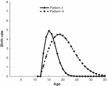
The two age-dependent female reproductive patterns, I and II, employed in our model, shown as the birth rate b(a), i.e., the average number of eggs produced per female per day. For each pattern, insects are classified into 35 age classes: 10 immature age classes and 25 adult age classes. The functional forms of these patterns are provided by truncated Weibull distributions. More precisely, we assume that b(a) = 0 for a ≤ 12 and 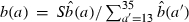for a ≥ 13. Here , for a ≥ 13. S is the total number of eggs that a female produces in her lifetime if she survives to the maximum age. In reproductive pattern I, S = 25 and λ = 4.4. In reproductive pattern II, S = 50 and λ = 9.5. Note that the larger the parameter λ is, the broader the reproductive interval.

For mosquitoes such as Aedes aegypti, females usually mate only once, and occasionally can mate more than once in their lifetime (Foster and Lea 1975; Williams and Berger 1980; Young and Downe 1982). In this paper, we assume that females mate only twice in their entire lifetime. The first mating occurs when adults just emerge (i.e., at age 11), while the second mating occurs 10 days after the first mating (i.e., at age 21) when the majority of a cohort has already died. We assume perfect sperm precedence by the last male to mate. As can be seen in Fig. 1, for reproductive pattern I a female's fecundity is very low by 10 days after her first mating, so the genes of males involved in the second mating are barely represented in the next generation.

Let N(G,a,t) and N^*(G,a,t) be the number of females and the number of males of age a and genotype G at time t, respectively. We assume a 1:1 sex ratio at birth and that survival is sex- and genotype-independent. The age and genotype-specific numbers of the female population can be tracked by the following deterministic recursive equations:

(1)

(2)

The dynamics of the male population can be tracked by the same set of equations with N(G,a,t) being replaced by N^*(G,a,t). The total number of viable eggs of genotype G produced by adults at time t, B(G,t), can be expressed as

(3)

Here f_e(G,J,K) measures the viability and relative fitness (i.e., survival probability) of a G-egg produced by a J-mother and K-father, as discussed in the previous section. Pr(G|J,K) is the probability that a zygote has genotype G when the parental genotypes are J and K, respectively. In the case of Mendelian segregation, this probability can be easily calculated by a computer algorithm. B₁(J,K,t) is the total number of eggs produced by females of genotype J who mated with males of genotype K, which can be further expressed as

(4)

Here, b(a) is the average number of eggs produced per day per female of age a, as discussed above. β(a,K,t) is the probability that a female of age a at time t mates with a male of genotype K. ψ(a,t^′) is the probability that a female of age a last mated t^′ days ago. For the two-occasion mating discussed earlier, we have that ψ(a,a − 11) = 1 for 11 ≤ a ≤ 20, ψ(a,a − 21) = 1 for a ≥ 21, and ψ(a,t^′) = 0 otherwise. For the multiple/everyday mating we have that ψ(a,0) = 1 and ψ(a,t^′)=0 for a ≥ 11 and t^′ > 0. The number of adult age classes is m (=25) and so the maximum time t^′ that can have elapsed since an individual was mated is m − 1 days. Notice that a female of age a at the current time t who last mated t^′ days ago would then have been of age a − t^′ and that the time then would have been t − t^′.

In this paper we assume that mating is random with respect to genotype, but is potentially assortative with respect to age. Females choose their mates with probability weighted by a mating preference function Φ(x) that depends on the age difference x between the female and a given male. In order to model different degrees of assortative mating we take Φ(x) to have the form

(5)

Here, 0 ≤ q ≤ 1 is a parameter by which we can adjust the degree of assortative mating. (For the situation in which q = 0, we adopt the notational convention that 0⁰ = 1.) The maximum possible age difference between male and female at mating is m − 1.

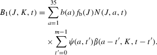
For a fixed 0<q<1, Φ(x) is a strictly decreasing function of x, which means that the mating preference decreases as the age difference increases. When q = 0, Φ(0) = 1 and Φ(x) = 0 for any x > 0, mating is completely assortative. When q = 1, Φ(x) = 1/m is constant for all x, mating is random. In this paper we consider five mating preference patterns for which q = 1, 0.94, 0.875, 0.75, and 0, respectively. The five mating patterns (MP), for which the degrees of assortative mating by age vary from being random mating to being completely assortative, are denoted by MP-1 through MP-5 (Fig. 2).

Figure 2.

Graphs of the five mating preference patterns, Φ(x), where x is the age difference between a male and a female. The five patterns represent different degrees of mating preference varying from random to completely assortative by age, which are denoted by MP₁, MP₂, MP₃, MP₄ and MP₅, respectively.

In terms of the mating preference function, we find that the mating function β(a,K,t) is given by

(6)

where the sums are only taken over adult age classes.

We consider a one-time introduction of homozygous engineered individuals, i.e., genotype aabb in the case of EU and genotype MM in the case of Medea. We consider three specific age-related introduction methods: (i) Single-age introduction, where all introduced engineered individuals have the same age; (ii) Two-age introduction, where equal numbers of engineered individuals from two different age classes are introduced; (iii) All-age introduction, where engineered individuals from all age classes are introduced, but with the same age distribution as the existing wild-type population. We assume that no introduced female has been mated prior to introduction. (We remark that this leads to a minor modification in the above model equations as the mating history of introduced and pre-existing females must be tracked separately until sufficient time has passed for the introduced cohort to have died.) We assume that introductions are made into a wild-type population that has attained its stable age distribution. In the simulations, we find this distribution by running the model for a sufficiently long time. All results presented in this paper were obtained numerically using a C++ simulation code (available on request from the authors).

Results

In the case of EU, the age-structured model has two stable equilibria E_s1 and E_s2, where the frequency of the wild genotype is 1 (constructs are lost) and at some low level (constructs are at high frequency), respectively. When there is no fitness cost (c = 0) the frequency of the wild genotype at E_s2 is 0 (constructs are fixed). The frequency of wild genotype at E_s2 increases as c increases. The age-structured model also has an unstable equilibrium, the location of which determines (in a nontrivial way) the introduction threshold. When the initial introduction frequency is below the threshold, the system approaches the E_s1 equilibrium and the wild-type goes to fixation. When the initial introduction frequency is above the threshold, the system approaches the E_s2 equilibrium, at which the frequency of the wild genotype is at some low level. The wild-type frequency is lower than 0.05 when the fitness cost c is lower than or equal 0.25.

In the case of Medea, the age-structured model has two stable equilibria at which the frequencies of the wild genotype are 1 and 0, respectively. When there are fitness costs associated with the Medea construct, the age-structured model has a unstable equilibrium whose location determines the introduction threshold. When the initial introduction frequency is below the threshold, the wild-type goes to fixation. When the initial introduction frequency is above the threshold, the wild genotype goes extinct.

Equilibrium genotype frequencies in the age-structured model are the same as those in the corresponding nonage-structured model. This result stems from our assumption that genotype-specific fitness effects (i.e., fecundity differences and survival probability differences) only occur at reproduction and at the embryonic stage, but not as individuals move between the various age classes. Consequently, at equilibrium each age class has the same genotype frequency distribution and so these equilibrium frequencies are identical to those in the nonage-structured model.

In the following sections we focus on the introduction thresholds to examine the effects of age structure. Introduction thresholds presented below are found numerically based on whether the long-term frequency of wild genotype is close to 1 or close to 0. Introduction threshold will be calculated as the proportion of released number of insects relative to the total population (including all age classes, both immature and adult) unless mentioned otherwise.

Single-age introduction of both sexes

In the case of EU, the introduction threshold varies considerably with the age of the introduced individuals. Compared with the introduction threshold predicted by the nonage-structured model, the threshold is relatively high for the introduction of a single age class of immature individuals or old adult individuals and relatively low for the introduction of a single age class of young adult individuals (Fig. 3A,B). For example, when there is no fitness cost, the nonage-structured model predicts a threshold of 27%, but the age-structured model with reproductive pattern I predicts a threshold of 13% for the introduction of age class 13 and a threshold of 75% for the introduction of age class 25.

Figure 3.

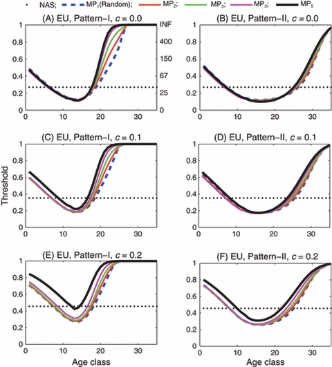
Engineered underdominance: Introduction threshold versus age class for the single-age introduction of both males and females. In panels (A), (C) and (E), the reproductive pattern is I and the fitness cost c is 0, 0.1 and 0.2, respectively. In panels (B), (D) and (F), the reproductive pattern is II and the fitness cost c is 0, 0.1 and 0.2, respectively. In each panel the horizontal dotted line is the threshold predicted by the nonage-structured model (labeled as NAS). The remaining five curves labeled by MP₁ through MP₅ are the age-specific thresholds corresponding to random, slightly assortative, moderately assortative, very assortative and completely assortative mating by age, respectively. In each panel, the left-hand vertical axis gives the threshold in terms of the proportion of introduced insects relative to the total population, whereas the right-hand vertical axis gives the threshold in terms of the number of introduced insects per 100 wild-type insects (INF means infinity).

In broad terms, the threshold is inversely related to the reproductive value of the introduced individuals (Fisher 1930; Gotelli 2001). We attempted to more specifically relate the introduction threshold to reproductive value, but found that this was not possible because calculation of reproductive value is based only on females, and males do not have the same reproductive value as females unless mating is completely assortative by age. Furthermore, reproductive value is altered by the introduction itself and the limited number of matings. While it is still useful to analyze the qualitative relations between the introduction threshold and reproductive value, a quantitative analysis is not possible. ‘Further details regarding the application of the reproductive value concept to models such as the one presented here will appear elsewhere (A.L. Lloyd, unpublished data).’

We assumed that females could only mate twice based on empirical data on mosquitoes. Under this assumption, previously emerged wild adult females in the natural population have already mated with wild-type males before the introduction of engineered insects and they do not mate again until up to 10 days after the introduction. In other words, the only wild-type females that can mate at the time of introduction are those newly emerged ones. Compared to the implicit assumption of unlimited multiple mating in the simple nonage-structured model, the sexual nonreceptivity of wild-type females at the time of introduction limits the production of heterozygous offspring that will contribute to gene-drive in the subsequent generation. Therefore, for the introduction of old adults, this limitation on mating generally causes higher thresholds than unlimited multiple/everyday mating. This has been verified by systematic comparisons between the thresholds for two-occasion and multiple-mating (results not shown). For example, if the reproductive pattern I, there is no fitness cost, and the introduced insects are 22 days old, then the thresholds assuming two-occasion mating and unlimited multiple-mating are 48.8% and 43.5%, respectively. The difference is greater when mating is assortative by age and/or when the introduced insects are older.

Mating preference has little impact on the introduction threshold for immature or young adult age classes. The situation is different, however, for the introduction of an old adult age class because, depending on the MP, older males and females can make quite different contributions to the offspring pool. Older females have very low fecundity, and if mating is assortative then older males correspondingly contribute little to the offspring pool. As the degree of assortativity of mating decreases, older males increasingly mate with younger females and hence benefit from their higher fecundity. As a consequence, when mating is anything other than totally assortative, older males can contribute more to gene-drive than older females, and so introduction thresholds decrease as the degree of assortativity decreases. When mating is random, older males frequently mate with young females and so the introduction threshold can be considerably lower than under strong assortative mating.

The introduction threshold increases as the fitness cost c increases (Fig. 3C–F). However, even if the fitness cost is as high as 20% the thresholds for the introduction of an immature or a young adult age class do not differ significantly among different mating preference patterns unless mating is almost completely assortative by age.

In reproductive pattern I, females have very low fecundity when they are older than 20 days (Fig. 1), so the threshold for the introduction of an age class larger than 20 is very high (Fig. 3A,C,E). In reproductive pattern II, females of age 20 still have rather high fecundity (Fig. 1), so the threshold for the introduction of age class 20 is very low compared with that in reproductive pattern I (Fig. 3B,D,F). The impact of assortative mating on the threshold in reproductive pattern I is stronger than in reproductive pattern II. This is partially due to the different contributions of males between the two reproductive patterns.

In the case of Medea, when a single age class of Medea males and females are introduced, the degree of assortative mating by age has a similar impact on the introduction thresholds as seen in the case of EU, except that the general threshold levels are much lower (Fig. 4).

Figure 4.

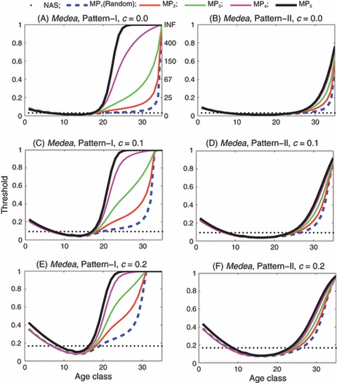
Medea: Introduction threshold versus age class for the single-age introduction of both males and females. In this figure, the fecundity loss of a homozygous Medea female is s = 0.1. In panels (A), (C) and (E), the reproductive pattern is I and the fitness cost c is 0, 0.1 and 0.2, respectively. In panels (B), (D) and (F), the reproductive pattern is II and the fitness cost c is 0, 0.1 and 0.2, respectively. In each panel, the dotted line is the threshold predicted by the nonage-structured model. The remaining five curves labeled by MP₁ through MP₅ are the age-specific thresholds corresponding to random, slightly assortative, moderately assortative, very assortative and completely assortative mating by age, respectively.

In addition to their threshold levels, EU and Medea differ in the extent to which the threshold is affected by age structure. To show this we focus on the minimum numbers of insects that must be introduced per 100 wild-type individuals which is an alternative way to express the threshold. In the case of EU, when mating is random, the absolute differences in the minimum numbers of insects that must be introduced per 100 wild-type individuals between the age-structured model (for the introduction of age class 13) and the simple nonage-structured model are 22.4, 30.1 and 46.4 for c = 0, 0.1 and 0.2, respectively (Table 1). If the target population has one million insects, then for c = 0.2, the simple model suggests that 464 000 more insects would have to be introduced than would be predicted by the age-structured model. From a practical perspective, this is a big difference. In the case of Medea, the absolute differences in the introduction thresholds between the age-structured model and the simple nonage-structured model are 1.8, 5.8 and 11.5 per 100 wild-type individuals for c = 0, 0.1 and 0.2, respectively. Compared to the case of EU, the differences between the simple model and the age-structured model are much smaller.

Table 1.

Comparisons of the introduction thresholds between the nonage-structured model (NAS) and the age-structured model (for the introduction of age class 13). Mating is random. The thresholds are given as the number of introduced insects per 100 wild-type insects

	EU (c = 0)	EU (c = 0.1)	EU (c = 0.2)
Threshold (NAS)	36.8	54.8	84.2
Threshold (age 13)	14.4	24.7	37.8
Difference	22.4	30.1	46.4
	Medea (c = 0)	Medea (c = 0.1)	Medea (c = 0.2)
Threshold (NAS)	3.2	10.1	20
Threshold (age 13)	1.4	4.3	8.5
Difference	1.8	5.8	11.5

Single-age introduction of only males

In the case of a male-only introduction of EU insects, the introduction thresholds are generally higher than those for the corresponding introduction of both males and females (Fig. 5). As in the case of both-sex introductions, the introduction threshold varies considerably with the age of the introduced individuals, and can be much lower or higher than that predicted by the nonage-structured model. For example, when there is no fitness cost, the nonage-structured model predicts a threshold of 38%, but the age-structured model with reproductive pattern I predicts a threshold of 29% for the introduction of age class 13 and a threshold of 62% for the introduction of age class 25. Note that in reproductive pattern I, males of age 25, as they can mate with younger females, have much larger contributions to gene-drive than females of the same age, so the introduction of only males of age 25 results in a lower threshold than the introduction of both males and females. Thresholds differ between reproductive patterns I and II, but the differences are not as substantial as they were for the introduction of both males and females.

Figure 5.

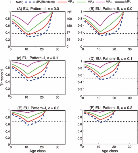
Engineered underdominance: Introduction threshold versus age class for the single-age introduction of only males. In panels (A) through (F), only males are introduced. Reproductive pattern is I in panels (A), (C) and (E), and II in panels (B), (D) and (F). Fitness cost c is 0 in panels (A) and (B), 0.1 in (C) and (D) and 0.2 in (E) and (F). In each panel the horizontal dotted line is the threshold predicted by the nonage-structured model (labeled as NAS). The remaining five curves labeled by MP₁ through MP₅ are the age-specific thresholds corresponding to random, slightly assortative, moderately assortative, very assortative and completely assortative mating by age, respectively. Note that for completely assortative mating by age (MP₅), the introduction thresholds are 1 for any age class, i.e., successful introduction is not possible. (This means that the black solid line is on the top of the frame in each panel.)

The degree of assortative mating by age has a great impact on the introduction thresholds, especially when the fitness cost is high. This is largely due to the limited mating of the F₀ wild-type adult females with the introduced males, as discussed in the previous subsection. In the case of male-only introduction, the negative impact of this mating limitation imposed by wild-type adult females on gene-drive is even stronger than in the case of both-sex introduction because only the wild-type females that mate with the introduced males can pass the engineered alleles to the next generation and contribute to gene-drive. In the worst case, i.e., when mating is completely assortative by age, the introduction of only males never achieves gene-drive, regardless of how many males are introduced (Fig. 5A–F).

In the case of a male-only single age-class introduction of Medea insects, the degree of assortative mating by age has a similar impact on the introduction thresholds as seen in the case of EU: the stronger the assortative mating is, the higher the threshold (Fig. 6). However, there are important differences between EU and Medea: (i) when mating is random, the threshold for the introduction of Medea males of age 25 is lower than 0.2 even when the fitness cost is as high as 0.2 (Fig. 6A–F), which is in contrast to the impossibility of achieving gene-drive with the introduction of EU males of the same age; (ii) when mating is random or slightly assortative by age and when the introduced insects are Medea adults, the introduction thresholds for the only-male introduction are almost always lower than those for the both-sex introduction (Figs 4 and 6). This is in contrast to the case of EU where the introduction thresholds for the only-male introduction are almost always higher than those for the both-sex introduction (Figs 3 and 5).

Figure 6.

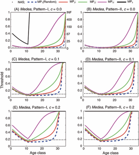
Medea: Introduction threshold versus age class for the single-age introduction of only males. In panels (A) through (F), only males are introduced. Reproductive pattern is I in panels (A), (C) and (E), and II in panels (B), (D) and (F). Fitness cost c is 0 in panels (A) and (B), 0.1 in (C) and (D) and 0.2 in (E) and (F). the fecundity loss of a homozygous Medea female is s = 0.1.

Two-age introduction

In order to determine whether there are differences between the introduction of a single age class and multiple age classes, we examine introductions involving two age classes. For illustration, we choose two age classes that have similar introduction thresholds in the case of single-age introduction when there are no fitness costs. (In order to make sure that the thresholds for the two age classes are as close as possible, the two age classes are chosen differently in some cases.)

In the case of EU, for reproductive pattern I, the introduction of both males and females of either age 9 or 17 results in a similar introduction threshold when there is no fitness cost (c = 0) and when mating is slightly assortative by age (with MP-2). When the fitness cost varies from 0 to 0.25, the thresholds for the simultaneous introduction of both age classes just differ slightly from the thresholds for the single-age introduction (Fig. 7A). Similar results are observed for reproductive pattern II where the two age classes chosen for examination are 9 and 24 (Fig. 7B).

Figure 7.

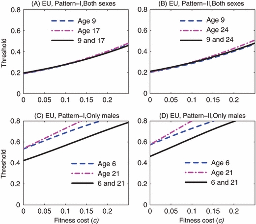
Engineered underdominance: Comparisons between the single-age introductions and two-age introduction. In panels (A) and (B), both males and females are introduced, while in panels (C) and (D), only males are introduced. In panels (A) and (C), the reproductive pattern is I, while in panels (C) and (D), the reproductive pattern is II. In each panel, the dashed line and the dot-dashed line illustrate the thresholds for the single-age introductions, while the solid line gives the thresholds for the two-age introduction. Note that in each panel the two age classes are chosen such that they result in similar introduction thresholds in the case of single-age introduction when there is no fitness cost, so these two age classes are not always the same among the four panels. In all panels, mating is assumed to be slightly assortative by age (i.e., MP₂ illustrated in Fig. 2).

In the case of Medea, for reproductive pattern I, the introduction of both males and females of either age 9 or 17 also results in a similar introduction threshold when there is no embryonic fitness cost (c = 0) and when mating is slightly assortative by age. The threshold for the introduction of both age classes together is very similar to those for the single-age introductions even when c is 0.25 (Fig. 8A). Similar results are observed for reproductive pattern II where the two age classes chosen for examination are 9 and 23 (Fig. 8B).

Figure 8.

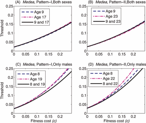
Medea: Comparisons between the single-age introductions and two-age introduction. In panels (A) and (B), both males and females are introduced, while in panels (C) and (D), only males are introduced. In panels (A) and (C), the reproductive pattern is I, while in panels (C) and (D), the reproductive pattern is II. In each panel, the dashed line and the dot-dashed line illustrate the thresholds for the single-age introductions, while the solid line gives the thresholds for the two-age introduction. In all panels, mating is assumed to be slightly assortative by age (i.e., MP₂ illustrated in Fig. 2).

In contrast, when only males are introduced there are significant differences between the single-age and two-age introductions. In the case of EU, the age-structured model for the two-age introduction predicts much lower thresholds than for the single-age introductions (Fig. 7C,D). In the case of Medea, the age-structured model for the two-age introduction also predicts lower thresholds than for the single-age introduction, but the differences are not so great as in the case of EU (Fig. 8C,D). These differences between the thresholds are largely due to the differences in the chances of mating between the wild-type adult females and the introduced males at the time of introduction. When the introduced males are of the same age, they compete for the same wild-type females that are available for mating at the time of introduction. When the introduced males are of two distinct ages, the degree of competition is reduced. The degree of competition increases as the number of introduced males increases, and that is why differences are small when the thresholds are lower, as seen in the case of Medea.

All-age introduction

In order to compare the age-structured model with the simple nonage-structured model under the same initial conditions, we examined the age-structured model in the case of all-age introduction (where the number of introduced insects is proportional to the number of wild insects with the same age). When both males and females are introduced, similar results are observed for EU and Medea: the introduction thresholds predicted by the age-structured model are slightly higher than those predicted by the simple model with the same value of the fitness cost. The differences in the thresholds become somewhat larger as c increases (Figs 9A,B and 10A,B). The higher thresholds in the age-structured model are largely due to the limited mating of the F₀ wild-type adult females, as discussed earlier.

Figure 9.

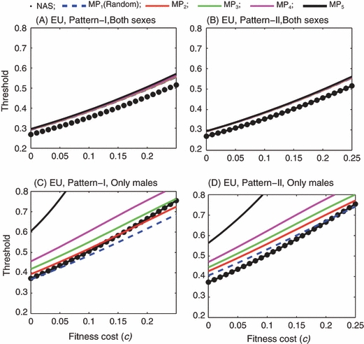
Engineered underdominance: Introduction thresholds as functions of fitness cost in the case of all-age introduction. In panels (A) and (B) both males and females are introduced. In panels (C) and (D) only males are introduced. In each panel, the thick dotted line is predicted by the simple nonage-structured model. The remaining five curves labeled by MP₁ through MP₅ correspond to the five mating preference patterns: random mating through completely assortative mating.

Figure 10.

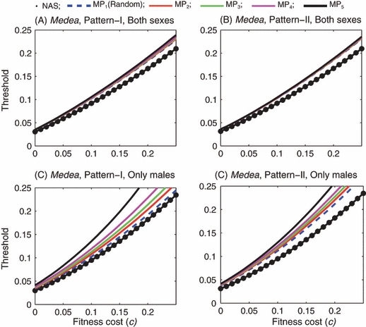
Medea: Introduction thresholds as functions of fitness cost in the case of all-age introduction. In panels (A) and (B) both males and females are introduced. In panels (C) and (D) only males are introduced. In each panel, the thick dotted line is predicted by the simple nonage-structured model. The remaining five curves labeled by MP₁ through MP₅ correspond to the five mating preference patterns: random mating through completely assortative mating.

When only males are introduced, the two-occasion mating of females has similar effects: during the initial period following the introduction, only those newly emerged adult wild-type females can mate with the introduced males and produce heterozygous offspring. Therefore, in the cases of EU and Medea the age-structured model predicts higher introduction thresholds than the nonage-structured model as long as the fitness cost is not very high (Figs 9C,D and 10C,D). However, when c is high and mating is random the age-structured model predicts lower introduction thresholds than the nonage-structured model in the case of EU (Fig. 9C,D).

When mating is random and only males are introduced, the age-structured model always predicts lower thresholds than the nonage-structured model as long as females mate every day and the introduction includes all age classes (Fig. 11). For example, when there is no fitness cost the threshold predicted by the age-structured model is about 33%, which is lower than the 38% predicted by the nonage-structured model. This is because in the nonage-structured model, males can only mate with females that are from the same discrete, nonoverlapping generation, while in the age-structured model with random mating, some males from the release generation survive long enough to mate with young females from the next generation. When mating occurs only twice instead of every day, the introduction thresholds predicted by the age-structured model increase, but they are still lower than those predicted by the nonage-structured model in cases where the fitness cost is high. Note that the fitness cost causes greater increases in thresholds in a nonage-structured population than in an age-structured population. It is also interesting that the age-structured model with complete assortative mating by age predicts almost the same thresholds as the nonage-structured model does.

Figure 11.

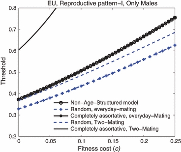
Engineered underdominance: Comparisons of the introduction thresholds among the nonage-structured model, the age-structured model with double-mating and the age-structured model with everyday-mating. In both the age-structured model and the nonage-structured model, only males are introduced. In the age-structured model, the introduction method is all-age introduction and the reproductive pattern is I. The two thicker lines with markers are the thresholds under the assumption of everyday-mating, while the two thinner lines with no markers are the thresholds under the assumption of two-mating. Note that the line corresponding to the nonage-structured model overlaps the line corresponding to the age-structured model when mating is completely assortative by age and occurs everyday.

Conclusions and discussion

In this study we used an age-structured genetic model to analyze the effects of age and mating-related factors on the number of engineered insects that must be introduced into a wild population to achieve successful gene-drive. In general, the introduction thresholds are lowest when young adults are introduced because they have the highest reproductive potential. When both males and females are introduced, assortative mating by age has little impact on the introduction threshold unless the introduced females are old, with diminished reproductive ability. Because males do not transmit disease, it has been recommended that only males be used in any introduction of engineered mosquitoes (Klassen and Curtis 2005). In general, male-only introductions increase introduction thresholds. For such introductions, even slight assortative mating by age can cause this increase to be dramatic. Even when there are no fitness costs and mating is random, the introduction of males 15 days after their emergence as adults cannot result in success of the EU approach. Previous models of EU and Medea drive mechanisms have not accounted for age structure and age-related mating details, and can overestimate or underestimate the numbers of engineered insects that must be introduced.

In this paper we have selected two specific gene-drive mechanisms as examples to examine the impact of age structure and age-related factors: Medea and EU. Medea achieves gene-drive by maternal-effect lethality to the offspring of Medea mothers that do not inherit a Medea allele from their mother or father. For EU, lethality occurs when an embryo inherits just one of the two co-dependent constructs, but involves no maternal effects. Although these two mechanisms are different, most results concerning the impact of age structure and age-related factors for the two mechanisms are similar, except that the general introduction threshold levels for EU are much higher than for Medea.

For both gene-drive mechanisms, Medea and EU, there are no deaths of first generation offspring from a cross between homozygous engineered insects and wild-type insects, so the gene-drive typically does not start until the second generation. Any population factors that decrease the percentage of matings between the engineered strain and the wild-type strain in the release generation will slow the onset of drive. When there are fitness costs, this will decrease the frequency of engineered alleles that are present in the second generation. Compared with random mating, assortative mating by age directly reduces the percentage of the engineered insects that mate with wild-type insects in the case of single-age introduction and so increases the thresholds. Compared with unlimited multiple mating, limited two-occasion mating and the fact that the wild-type adult females have mated with wild-type males before release also reduce the percentage of matings between the engineered insects and the wild-type insects, and this causes higher thresholds in the age-structured model than in the nonage-structured model.

Introduction of only transgenic male mosquitoes is generally considered more socially acceptable than the introduction of males and females because males do not bite humans and therefore do not transmit disease (Klassen and Curtis 2005). Male-only introductions (and introductions involving unmated sexually mature females) require the ability to sex insects on a large scale. There have been successful examples of separating mosquitoes by sex, e.g., according to pupal size or using genetic techniques (Klassen and Curtis 2005). However, as demonstrated in this paper, male-only introduction generally cause higher thresholds than both-sex introduction. It must also be understood that unless there is a way of causing death of female eggs in the last generation of factory-reared transgenic insects, the rearing cost associated with release of one transgenic male is expected to approach the cost of releasing one male and one female. The benefit of achieving the more socially acceptable approach of male-only release may far outweigh issues associated with critical thresholds and rearing costs, but these factors should at least be considered.

While we have demonstrated that age structure, mating behavior and fitness costs could work in combination to affect the population dynamics of gene-drive, we lack detailed field studies in these aspects. Based on the results of our model, it would be useful, but not critical to study the extent of assortative mating by age if both males and females are expected to be used in the introductions. However, if a male-only introduction is anticipated, knowledge of the degree of assortative mating would be essential. In our simulations, there was only a minor impact from the second mating (data not shown). However, if the lifespan and reproductive period of females were longer, the second mating could be more important. Given that these parameters vary between species and even from population to population, our results emphasize the need for detailed field studies of these parameters before predictions can be made about the numbers and ages of engineered insects to introduce in a specific situation.

Appendix A

The basic population genetic model of engineered underdominance

We consider introduction of engineered insects homozygous for two co-dependent engineered constructs inserted into two nonhomologous autosomes, a and b. The introduced genotype and the wild-type are denoted as aabb and AABB, respectively. We assume that (i) generations are nonoverlapping; (ii) mating is random; (iii) sex ratio in F₁ and later generations is 1:1.

When the engineered individuals cross with the wild-type individuals, there are four types of mating in the F₀ generation: female AABB × male AABB, female AABB × male aabb, female aabb × male AABB, female aabb × male aabb. These four types of matings lead to three genotypes in the F₁ generations: AABB, AaBb and aabb which are all viable. In the case of random mating the frequencies of the three viable genotypes in the F₁ generation, (AABB)₁, (AaBb)₁ and (aabb)₁, can be calculated by the following equations:

(A.1)

(A.2)

(A.3)

Here,

(A.4)

is the mean fitness. The subscripts m0 and f0 represent the genotype frequencies in males and females, respectively. f₀₀ = 1 and f₂₂ = (1 − c)² are the fitnesses of the genotypes AABB and aabb, respectively. Note that because we assume a 1:1 sex ratio for offspring, in the F₁ and later generations genotype frequencies in males and females are the same. Therefore, we will drop the sex-specific subscripts from the genotype notation from F₁ generation.

In the F₂ and later generations there are nine genotypes: AABB, AABb, AaBB, AaBb, AAbb, aaBB, Aabb, aaBb and aabb. Among them only five are viable: AABB, AaBb, Aabb, aaBb and aabb. The other four genotypes are not viable because they contain only construct a or b. In Mendelian segregation the frequencies of gametes (AB), (Ab), (aB) and (ab) in the next generation (represented by a prime) can be calculated by the frequencies of genotypes of the current (F₁ or later) generation as follows

(A.5)

(A.6)

(A.7)

(A.8)

Here f₀₀ = 1, f₁₁ = (1 − c/2)², f₁₂ = f₂₁ = (1 − c/2) (1 − c), f₂₂ = (1 − c)² are the fitnesses of the five genotypes AABB, AaBb, Aabb, aaBb and aabb, respectively. Note that the fitness costs of constructs a and b are assumed to be the same. W is the sum of all numerators on the right-hand side of Eqns (A.5)–(A.8). In the case of random mating, the relative frequencies of the five viable genotypes can be calculated based on the frequencies of gametes:

(A.9)

(A.10)

(A.11)

(A.12)

(A.13)

Substitution of Eqns (A.9)–(A.13) into Eqns (A.5)–(A.8) eliminates the genotype frequencies and leaves a system of four equations for the gamete frequencies.

Because we consider the introduction of homozygous genotype aabb to a wild population with genotype AABB, initially (Ab) = (aB) = 0. As long as this relation initially holds, it is easy to check that (Ab)=(aB) always holds. Using this symmetry between a and b and the condition (AB) + (aB) + (Ab) + (ab) = 1, this set of four equations reduces to just two

(A.14)

(A.15)

Here . When c = 0, the model has three equilibria, two locally stable ones: E_s1: (AB,ab) = (0,1) (constructs are fixed) and E_s2:(AB,ab) = (1,0) (constructs are lost) and an unstable one E_u: (AB,ab) ≍ (0.63,0.17). When c > 0 the equilibrium values at E_s2 are the same as for c=0, but the equilibrium values at E_s1 and E_u depend on c. Generally it is hard to derive analytical expressions for these two equilibria. Numerically we find that at E_s1, AB increases as c increases, but ab decreases as c increases. When c = 0.25 the equilibrium values (AB,ab) ≍ (0.02,0.76) at E_s1.

All numerical results concerning the introduction thresholds in the nonage-structured model are based on numerical simulation of the model.

Appendix B

The basic population genetic model of Medea

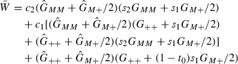
Let G_MM, G_M+ and G₊₊ be the frequencies of females of genotypes MM, M+ and ++, respectively. Let , and be the frequencies of males of genotypes MM, M+ and ++, respectively. Based on Wade and Beeman (1994), the genotype frequencies in the offspring generation after selection (represented by a prime) are

(B.1)

(B.2)

(B.3)

(B.4)

Here c₁ = 1 − c/2 and c₂ = 1 − c are the embryonic fitnesses of M+ and MM, respectively. While s₁ = 1 − s/2 and s₂ = 1 − s are the fecundity fitnesses of the M+ and MM adult females, respectively. t₀ is the mortality of wild-type offspring produced by females carrying the Medea allele(s). In our model, the maternal fecundity loss s = 0.1, and the maternal-effect mortality t₀ = 1 are fixed. c is allowed to vary from 0 to 0.25.

After the F₀ generation the sex ratio is assumed to be 1:1, so the genotype frequencies in males and females are the same. This means that we do not have to distinguish between and G. Noticing that G_MM + G_M+ + G₊₊ = 1 the set of three Eqns (B.1)–(B.3) can be reduced to only two equations.

When s = c = 0 we find that the model has two equilibria: an unstable one E₀: (G_MM,G_M+,G₊₊) = (0,0,1), where the entire population is wild-type, and a stable one E₁: (G_MM,G_M+,G₊₊) = (1,0,0), where the wild genotype is eliminated. When s > 0 and/or c > 0 the model has three equilibria: two stable ones E₀ and E₁, and an unstable one E_u. The equilibrium E₀ is (0,0,1) which is independent of s and c. The equilibrium E₁ has the form (1 − q,q,0) in which 0 < q < 1 is a function of s and c. In general it is difficult to derive the expressions of q and the entries of E_u.

Literature cited

- Beeman RW, Friesen KS, Denell RE. Maternal-effect, selfish genes in flour beetles. Science. 1992;256:89–92. doi: 10.1126/science.1566060. [DOI] [PubMed] [Google Scholar]
- Burt A. Site-specific selfish genes as tools for the control and genetic engineering of natural populations. Proceedings. Biological Sciences/The Royal Society. 2003;270:921–928. doi: 10.1098/rspb.2002.2319. [DOI] [PMC free article] [PubMed] [Google Scholar]
- Burt A. Homing endonuclease genes: the rise and fall and rise again of a selfish element. Current Opinion in Genetics and Development. 2004;14:609–615. doi: 10.1016/j.gde.2004.09.010. [DOI] [PubMed] [Google Scholar]
- Burt A, Trivers R. Genes in Conflict: The Biology of Selfish Genetic Elements. Cambridge, U.K: Harvard University Press; 2006. [Google Scholar]
- Chen CH, Huang H, Ward CM, Su JT, Schaeffer LV, Guo M, Hay BA. A synthetic maternal-effect selfish genetic element drives population replacement in Drosophila. Science. 2007;316:597–600. doi: 10.1126/science.1138595. [DOI] [PubMed] [Google Scholar]
- Davis S, Bax N, Grewe P. Engineered underdominance allows efficient and economical introgression of traits into pest populations. Journal of Theoretical Biology. 2001;212:83–98. doi: 10.1006/jtbi.2001.2357. [DOI] [PubMed] [Google Scholar]
- Fisher R. The Genetical Theory of Natural Selection. New York: Dover; 1930. ‘reprinted 1958’. [Google Scholar]
- Foster WA, Lea AO. Renewable fecundity of male Aedes aegypti following replenishment of seminal vesicles and accessory glands. Journal of Insect Physiology. 1975;21:1085–1090. doi: 10.1016/0022-1910(75)90120-1. [DOI] [PubMed] [Google Scholar]
- Franz AWE, Sanchez-Vargas I, Adelman ZN, Blair CD, Beaty BJ, James AA, Olson KE. Engineering RNA interference- based resistance to dengue virus type-2 in genetically-modified Aedes aegypti. Proceedings of the National Academy of Sciences of the United States of America. 2006;103:4198–4203. doi: 10.1073/pnas.0600479103. [DOI] [PMC free article] [PubMed] [Google Scholar]
- Gotelli NJ. A Primer Of Ecology. Sunderland, MA: Sinauer Associates; 2001. [Google Scholar]
- Gould F, Magori K, Huang Y. Genetic strategies for controlling mosquito-borne diseases. American Scientist. 2006;94:238–246. [Google Scholar]
- Harrington LC, Edman JD, Scott TW. Why do female Aedes aegypti (Diptera: Culicidae) feed preferentially and frequently on human blood? Journal of Medical Entomology. 2001;38:411–422. doi: 10.1603/0022-2585-38.3.411. [DOI] [PubMed] [Google Scholar]
- Huang Y, Magori K, Lloyd AL, Gould F. Introducing desirable transgenes into insect populations using Y-linked meiotic drive: a theoretical assessment. Evolution. 2007;61:717–726. doi: 10.1111/j.1558-5646.2007.00075.x. [DOI] [PubMed] [Google Scholar]
- Ito J, Ghosh A, Moreira LA, Wimmer EA, Jacobs-Lorena M. Transgenic anopheline mosquitoes impaired in transmission of a malaria parasite. Nature. 2002;417:452–455. doi: 10.1038/417452a. [DOI] [PubMed] [Google Scholar]
- James AA. Gene drive systems in mosquitoes: rules of the road. Trends in Parasitology. 2005;21:64–67. doi: 10.1016/j.pt.2004.11.004. [DOI] [PubMed] [Google Scholar]
- Klassen W, Curtis CF. History of sterile insect technique. In: Dyck VA, Hendrichs J, Robinson AS, editors. Sterile Insect Technique: Principles and Practice in Area-Wide Integrated Pest Management. The Netherlands: Springer; 2005. pp. 3–36. [Google Scholar]
- Magori K, Gould F. Genetically engineered underdominance for manipulation of pest populations: a deterministic model. Genetics. 2006;172:2613–2620. doi: 10.1534/genetics.105.051789. [DOI] [PMC free article] [PubMed] [Google Scholar]
- McDonald PT. Population characteristics of domestic Aedes aegypti (Diptera: Culicidae) in villages on the Kenya Coast I. Adult survivorship and population size. Journal of Medical Entomology. 1977;14:42–48. doi: 10.1093/jmedent/14.1.42. [DOI] [PubMed] [Google Scholar]
- Rasgon JL, Scott TW. Impact of population age structure on Wolbachia transgene driver efficacy: ecologically complex factors and release of genetically-modified mosquitoes. Insect Biochemistry and Molecular Biology. 2004;34:707–713. doi: 10.1016/j.ibmb.2004.03.023. [DOI] [PubMed] [Google Scholar]
- Scott TW, Takken W, Knols BGJ, Boete C. The ecology of genetically modified mosquitoes. Science. 2002;298:117–119. doi: 10.1126/science.298.5591.117. [DOI] [PubMed] [Google Scholar]
- Sinkins SP, Gould F. Gene-drive systems for insect disease vectors. Nature Reviews. Genetics. 2006;7:427–435. doi: 10.1038/nrg1870. [DOI] [PubMed] [Google Scholar]
- Wade MJ, Beeman RW. The population dynamics of maternal-effect selfish genes. Genetics. 1994;138:1309–1314. doi: 10.1093/genetics/138.4.1309. [DOI] [PMC free article] [PubMed] [Google Scholar]
- Williams RW, Berger A. The relation of female polygamy to gonotrophic activity in the ROCK strain of Aedes aegypti. Mosquito News. 1980;40:597–604. [Google Scholar]
- Young ADM, Downe AER. Renewal of sexual receptivity in mated female mosquitoes, Aedes aegypti. Physiological Entomology. 1982;7:467–471. [Google Scholar]