

Abstract
Common garden studies are increasingly used to identify differences in phenotypic traits between native and introduced genotypes, often ignoring sources of among-population variation within each range. We re-analyzed data from 32 common garden studies of 28 plant species that tested for rapid evolution associated with biological invasion. Our goals were: (i) to identify patterns of phenotypic trait variation among populations within native and introduced ranges, and (ii) to explore the consequences of this variation for how differences between the ranges are interpreted. We combined life history and physiologic traits into a single principal component (PCALL) and also compared subsets of traits related to size, reproduction, and defense (PCSIZE, PCREP, and PCDEF, respectively). On average, introduced populations exhibited increased growth and reproduction compared to native conspecifics when latitude was not included in statistical models. However, significant correlations between PC-scores and latitude were detected in both the native and introduced ranges, indicating population differentiation along latitudinal gradients. When latitude was explicitly incorporated into statistical models as a covariate, it reduced the magnitude and reversed the direction of the effect for PCALL and PCSIZE. These results indicate that unrecognized geographic clines in phenotypic traits can confound inferences about the causes of evolutionary change in invasive plants.
Keywords: biogeographical comparisons, clinal variation, common garden, EICA, evolution of invasive species, introduced plants, latitudinal gradients
Introduction
Biological invasions are initiated by the transport of individuals from the native range of a species to the introduced range, where abiotic or biotic conditions may differ. The movement of propagules to new sites may create a mismatch between phenotypic traits and the environment. Hence, a fundamental issue for studies of introduced species concerns how important rapid evolution of local adaptation might be as a mechanism enabling persistence and spread in novel environments (Reznick and Ghalambor 2001; Sakai et al. 2001; Stockwell et al. 2003; Cox 2004; Lambrinos 2004; Barrett et al. 2008; Keller and Taylor 2008). Is rapid evolution of local adaptation within the introduced range essential for invasion success, or are pre-adaptation, phenotypic plasticity or other factors more important in enabling exotics to succeed in their adopted homes? Answers to these questions are of fundamental importance to our understanding of the ecology and evolution of plant invasions.
The likelihood of rapid, adaptive evolution occurring during invasion depends on both the amount of standing genetic variation in founding populations, and the relative importance of stochastic and deterministic forces operating during colonization. Although the process of local adaptation within introduced populations is difficult to measure, it can be inferred from a combination of common garden experiments and genetic analyses. However, because rigorous tests for rapid evolution of local adaptation in exotic populations are still infrequent, the prevalence of adaptive evolution during plant invasion remains unclear, despite repeated suggestions that invasive spread commonly involves rapid evolutionary change (e.g. Sakai et al. 2001; Müller-Schärer et al. 2004; Bossdorf et al. 2005).
Among ecologists, interest in determining the role of rapid evolution to invasion success has been motivated, in part, by observations that introduced species are often larger in size than their native counterparts (Crawley 1987; Grosholz and Ruiz 2003). If this pattern is the result of evolutionary change rather than, for example, plasticity, it could provide important insights into why invasive species are often able to dominate and out-compete natives in recipient communities. Blossey and Nötzold (1995) proposed a hypothesis to explain the evolution of increased size or fecundity evident in some introduced plant populations relative to natives (the ‘evolution of increased competitive ability’ or EICA hypothesis). This hypothesis posits that ‘invasiveness’ evolves due to escape from natural enemies. In the absence of specialist enemies, costly defense traits are reduced in introduced plants, thereby enabling gains in traits that increase competitive ability such as size or fecundity. EICA has now spawned many ‘common garden’ experiments; however, a recent tally of studies revealed only mixed support for the predictions of EICA (Bossdorf et al. 2005).
The common garden experiment is a classical approach to quantifying genetically based phenotypic differentiation among populations, particularly in sessile organisms like plants (reviewed in Langlet 1971). As EICA predicts that differences among native and introduced phenotypes are due to evolutionary responses within the introduced range, tests of this hypothesis require comparisons of native and introduced genotypes within common environments. However, observed differences in size or fecundity between native and introduced genotypes in a common garden do not provide unequivocal support for EICA. Comparisons between ranges can be complicated by significant among-population variation in traits within one or both ranges (Fig. 1). For example, if a particular phenotypic trait, such as size or reproduction, co-varies with latitude (i.e. there is clinal variation), then among-population variation can potentially complicate statistical comparisons between native and introduced populations. In principle, environmental clines in any phenotypic trait can increase the odds of finding significant differences between the native and introduced range for that trait. This can occur for at least three reasons: (i) when populations are insufficiently sampled, (ii) when native and introduced populations do not occupy a similar range of latitudes in both ranges, or (iii) when latitudes of native and introduced populations are matched, but the environment at a given latitude differs between the native and introduced range. In each case, differences in phenotype, such as size or reproduction, might appear to support an overall increase (or decrease) in competitive ability of introduced populations, when instead populations are merely adapted to abiotic conditions that correlate with latitude (Fig. 1).
Figure 1.
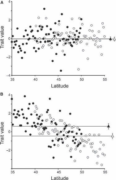
Simulated data for a standardized (i.e. mean = 0) phenotypic trait (e.g. biomass, seed set) to demonstrate the effect of latitude on inferred differences between native (open symbols) and introduced (closed symbols) populations. Circles represent population means; triangles denote average differences between ranges (i.e. native versus introduced), with 95% confidence intervals. (A) When no latitudinal clines are present there is no significant difference (P = 0.856) between the native and introduced ranges. (B) A parallel cline results in a significant difference (P < 0.0001) between ranges when latitude is not included in the statistical model; this difference is nonsignificant (P = 0.557) if latitude is included as a covariate. Seventy-five simulated population means from each range were drawn from a normal z-distribution (mean = 0, SD = 1), and populations represent an even sampling every 0.2° of latitude, from 40–55° in the native range and 35–50° in the introduced range. The slope of the gradient is −0.2 units per degree of latitude (B).
Environmental factors such as temperature, duration of growing season, and day length often vary in a predictable and continuous manner with latitude, and native plant populations frequently exhibit latitudinal clines in traits as a result of adaptive responses to this variation (i.e. local adaptation). Although rarely examined, genetically based latitudinal clines in traits related to growth, phenology and life history have been identified in introduced populations of several plant species (Weber and Schmid 1998; Kollmann and Bañuelos 2004,Maron et al. 2004b, 2007; Friedman et al. 2008; Montague et al. 2008). Latitudinal clines may be evident in a common environment even if field populations do not exhibit clines in situ. For example, latitudinal clines in growth and phenology can be contingent upon common garden conditions (Maron et al. 2004b; Bradshaw and Holzapfel 2008). Other environmental factors, like temperature or season length, can result in phenotypic gradients in common garden experiments that are not necessarily evident in situ (Conover and Schultz 1995).
The growing number of common garden studies of native and introduced plants provide an opportunity to determine how often clines occur in native and introduced populations, and whether trait differences between ranges (i.e. native versus introduced) are evident once any clinal patterns have been accounted for. Estimates from common garden experiments of the average difference in morphological, physiological or defensive traits between native and introduced ranges may be misleading if there is significant population divergence along environmental gradients that is not considered in sampling regimes or statistical analyses. Here, we focus our analysis on plants because of the available data from many common garden studies. However, our conclusions should apply broadly given that latitudinal gradients underlie the biogeographical ‘rules’ (e.g. Allen's Rule, Bergmann's Rule) identified in many studies of vertebrate, invertebrate, aquatic, marine and terrestrial animal species (see Connover and Schultz 1995; Huggett 2004).
In this study, we re-analyze raw data provided by authors of 47 common garden studies that compared traits among native and introduced conspecific plant populations. Our goal was to assess quantitatively how often there are: (i) genetically based differences in traits related to fitness between native and introduced populations (data available from 47 studies of 34 species), and (ii) latitudinal clines in traits among populations from either the native or introduced range (32 studies of 28 species). We then asked how the presence of latitudinal clines among native and/or introduced populations influenced estimates of trait differences between ranges, and how clines may affect tests of EICA. We hypothesized that clinal variation in plant traits might explain differences between native and introduced populations that have previously been used to support (or reject) EICA.
Methods
Data sources
We used a combination of web-based literature searches, personal communications, and examination of reference lists to identify common garden studies of plants in which phenotypes of individuals from native and introduced populations were compared. From these studies, we obtained or calculated population means for morphological, physiological, defense and life-history traits, as well as the latitude of sampled populations. In a few cases where original data could not be obtained directly from authors, we extracted means from published graphs and tables using image analysis software (Abramoff et al. 2004) and estimated latitudes using Google Earth. In total, we identified 54 studies (representing 43 species; Appendix A). In most (46 of 54), plants were grown in a single common garden usually located in the introduced range (27 of 46 studies; Table 1). In some cases, researchers imposed different treatments (e.g. herbivore treatment, fertilization; see Table S1) within the same common garden location. The species-weighted average study used 5.4 and 5.6 populations from the native and introduced range, respectively, and grew them in an average of 1.1 common garden locations.
Table 1.
Summary of common garden studies comparing phenotypic characteristics of native and introduced populations of plants
| Regions sampled* | Populations | Common garden(s)* | ||||||
|---|---|---|---|---|---|---|---|---|
| Ref. | Species | Native range | Introduced range | N | I | d.f. | N | Location(s) |
| 5† | Abutilon theophrasti | IND | USA | 2 | 1 | 1 | 1 | CO-USA (I) |
| 5† | Aegilops cylindrica | TUR, AFG | USA | 2 | 2 | 2 | 1 | CO-USA (I) |
| 6† | Alliaria petiolata | EUR (widespread) | USA (MA, IL, OH) | 8 | 7 | 13 | 1 | DEU (N) |
| 7† | Alliaria petiolata | EUR (widespread) | USA (MA, IL, OH, WI) | 8 | 8 | 14 | 1 | DEU (N) |
| 12† | Alliaria petiolata | GBR, NET | USA (OH, PA) | 7 | 4 | 9 | 1 | OH-USA (I) |
| 20 | Ambrosia artemisiifolia | USA (SC), CAN (ON) | FRA | 2 | 1 | 1 | 3 | ON-CAN (N); FRA x 2 (I) |
| 5† | Avena fatua | AFG, PAK | USA | 2 | 2 | 2 | 1 | CO-USA (I) |
| 9 | Barbarea vulgaris | DEU, AUT | USA (NE) | 2 | 3 | 3 | 1 | CHE (N) |
| 5† | Bromus tectorum | TUR | USA | 2 | 2 | 2 | 1 | CO-USA (I) |
| 9 | Bunias orientalis | DEU, AUT | USA (NE) | 2 | 3 | 3 | 1 | CHE (N) |
| 8† | Butomus umbellatus | CZE, FRA | NA (widespread) | 6 | 5 | 9 | 1 | ON-CAN (I) |
| 9 | Cardaria draba | DEU, AUT | USA (NE) | 2 | 3 | 3 | 1 | CHE (N) |
| 51 | Carduus nutans | GBR, DEU, FIN, ESP | AUS, NZE | 7 | 7 | 12 | 1 | GBR (N) |
| 5† | Centaurea diffusa | RUS, UKR | USA | 2 | 2 | 2 | 1 | CO-USA (I) |
| 5† | Centaurea maculosa | UKR | USA | 1 | 2 | 1 | 1 | CO-USA (I) |
| 13 | Centaurea solstitialis | ITA, ESP | USA (WA, ID, CA) | 2 | 6 | 6 | 1 | ITA (N) |
| 47† | Centaurea solstitialis | TUR, ITA, GRC, FRA, RUS | USA (CA, ID) | 13 | 8 | 19 | 2 | FRA (N), RUS (N) |
| 15† | Clidemia hirta | CRI | USA (HI) | 4 | 4 | 6 | 1 | HI-USA (I) |
| 48† | Cynoglossum officinale | DEU, HUN, NLD | USA (MO, WY, WA, ID), CAN (AB, BC) | 10 | 10 | 18 | 2 | DEU (N), MO-USA (I) |
| 5† | Desmodium tortuosum | BRA | IND | 2 | 2 | 2 | 1 | CO-USA (I) |
| 51 | Digitalis purpurea | GBR, FRA, DEU | AUS, NZE | 6 | 4 | 8 | 1 | GBR (N) |
| 5† | Echinochloa crus-galli | AFG, DEU | USA | 2 | 2 | 2 | 1 | CO-USA (I) |
| 51 | Echium vulgare | GBR, FIN, FRA, DEU | AUS, NZE | 6 | 6 | 10 | 1 | GBR (N) |
| 5† | Elytrigia repens | AFG, IND | USA | 2 | 1 | 1 | 1 | CO-USA (I) |
| 28† | Eschscholzia californica | USA (CA) | CHL | 7 | 4 | 9 | 1 | CA-USA (I) |
| 29† | Eschscholzia californica | USA (CA) | CHL | 12 | 10 | 20 | 1 | CA-USA (I) |
| 30 | Euphorbia esula | USA (MT, NE, ND, SD) CAN (MB) | AUT | 4 | 1 | 3 | 1 | ND-USA (I) |
| 31† | Hypericum perforatum | EUR (widespread) | USA (widespread), CAN (ON) | 19 | 32 | 49 | 4 | SWE & ESP (N); CA & WA-USA (I) |
| 32† | Hypericum perforatum | EUR (widespread) | USA (widespread), CAN (ON) | 17 | 32 | 47 | 2 | ESP (N); WA-USA (I) |
| 33† | Hypericum perforatum | EUR (widespread) | USA (OR, WA, CA) | 19 | 17 | 34 | 2 | ESP (N); WA-USA (I) |
| 46† | Hypericum perforatum | EUR (widespread) | USA, CAN (ON) | 10 | 20 | 28 | 1 | ESP (N) |
| 14† | Lepidium draba = Cardaria draba | HUN, DEU, ROM, UKR | USA (ID, OR, WA) | 10 | 10 | 18 | 1 | ID-USA (I) |
| 34 | Lepidium draba = Cardaria draba | HUN, ROM, ARM | USA (ID, OR, CO, NV, MT, WY) | 6 | 10 | 14 | 1 | CHE (N) |
| 36† | Lepidium draba = Cardaria draba | DEU, HUN, ROU | USA (WA, OR, ID) | 11 | 10 | 19 | 1 | DEU (N) |
| 5† | Lespedeza cuneata | CHN, IND | USA | 2 | 1 | 1 | 1 | CO-USA (I) |
| 5† | Leucanthemum vulgare | FIN, RUS | USA | 2 | 2 | 2 | 1 | CO-USA (I) |
| 5† | Linaria dalmatica | MKD, YUG | USA | 1 | 2 | 1 | 1 | CO-USA (I) |
| 1† | Lythrum salicaria | CZE | USA (IN) | 3 | 3 | 4 | 1 | WI-USA (I) |
| 3 | Lythrum salicaria | EUR (widespread) | USA (widespread) | 13 | 23 | 34 | 1 | NY-USA (I) |
| 4† | Lythrum salicaria | FRA | USA (NY) | 1 | 1 | 0 | 1 | DEU (N) |
| 11† | Lythrum salicaria | DEU | USA (IA, MN, NY) | 3 | 3 | 4 | 1 | IA-USA (I) |
| 49† | Lythrum salicaria | DEU, IRL, FIN, FRA | AUS (SE) USA (MD, NY, UT) | 6 | 4 | 8 | 2 | NY-USA (N) & GBR (N) |
| 50† | Lythrum salicaria | DEU, IRL, FIN, FRA | AUS (SE), USA (MD, NY, NE, SD) | 6 | 6 | 10 | 1 | GBR (N) |
| 18† | Melaleuca quinquenervia | AUS, NCL | USA (FL) | 8 | 10 | 16 | 1 | USA (I) |
| 19† | Melaleuca quinquenervia | AUS, NCL | USA (FL) | 8 | 10 | 16 | 1 | USA (I) |
| 25† | Melaleuca quinquenervia | AUS (E) | USA (FL) | 3 | 4 | 5 | 1 | NJ-USA (I) |
| 27† | Phalaris arundinacea | CZE, FRA | USA (VT, NC) | 2 | 2 | 2 | 1 | USA (I) |
| 5† | Poa annua | AFG, IND | CAN | 2 | 2 | 2 | 1 | CO-USA (I) |
| 17† | Rhododendron ponticum | GEO, ESP | IRL | 12 | 6 | 16 | 1 | DEU (N) |
| 9 | Rorippa austriaca | DEU, AUT | USA (NE) | 2 | 3 | 3 | 1 | CHE (N) |
| 26† | Sapium sebiferum = Triadica sebifera | CHN | USA (TX) | 1 | 1 | 0 | 1 | CA-USA (I) |
| 37† | Sapium sebiferum = Triadica sebifera | CHN | USA (TX) | 1 | 1 | 0 | 1 | TX-USA (I) |
| 38† | Sapium sebiferum = Triadica sebifera | CHN | USA (TX) | 1 | 1 | 0 | 1 | TX-USA (I) |
| 39† | Sapium sebiferum = Triadica sebifera | CHN | USA (TX) | 1 | 1 | 0 | 1 | TX-USA (I) |
| 40† | Sapium sebiferum = Triadica sebifera | CHN | USA (TX) | 1 | 1 | 0 | 1 | TX-USA (I) |
| 41† | Sapium sebiferum = Triadica sebifera | TWN | USA (GA, LA, TX) | 1 | 3 | 2 | 1 | USA (I) |
| 42† | Sapium sebiferum = Triadica sebifera | CHN, TWN | USA (GA, LA, TX) | 1 | 3 | 2 | 1 | TX-USA (I) |
| 43† | Sapium sebiferum = Triadica sebifera | CHN | USA (TX) | 2 | 1 | 1 | 2 | HI-USA & TX-USA (I) |
| 53† | Sapium sebiferum = Triadica sebifera | CHN | USA (TX) | 4 | 4 | 6 | 1 | CHN (N) |
| 54† | Senecio inaequidens | ZAF | DEU, CHE, FRA, NLD | 12 | 11 | 21 | 1 | NLD (I) |
| 24† | Senecio jacobaea | EUR (widespread) | USA & CAN (widespread), NZL, AUS | 14 | 16 | 28 | 1 | NLD (N) |
| 44† | Senecio jacobaea | NLD, FRA, CHE | USA (OR, MT), NZL | 4 | 4 | 6 | 1 | CHE (N) |
| 51 | Senecio jacobaea | GBR, DEU, FIN | AUS, NZE | 6 | 6 | 10 | 1 | GBR (N) |
| 10† | Senecio pterophorus | ZAF | ESP | 4 | 4 | 6 | 1 | ESP (I) |
| 22† | Senecio vulgaris | CHE | AUS, USA (CA, MT, NY OH, OR) | 8 | 16 | 22 | 1 | CHE (N) |
| 2 | Silene latifolia | EUR (widespread) | USA (E), CAN (BC, AB) | 20 | 20 | 38 | 1 | GA-USA (I) |
| 16 | Silene latifolia | EUR (widespread) | USA (E), CAN (BC, AB) | 15 | 19 | 32 | 1 | DEU (N) |
| 52† | Silene latifolia | EUR (widespread) | USA (E), CAN (BC, AB) | 20 | 20 | 38 | 1 | NLD (N) |
| 45† | Solidago canadensis | USA (E) | EUR (widespread) | 10 | 9 | 17 | 1 | CHE (I) |
| 21† | Solidago gigantea | USA | EUR (widespread) | 20 | 22 | 40 | 1 | DEU (I) |
| 23† | Solidago gigantea | USA | EUR (widespread) | 10 | 20 | 28 | 1 | WI-USA (N) |
| 35† | Solidago gigantea | EUR (widespread) | USA (widespread) | 20 | 10 | 28 | 1 | WI-USA (N) |
| 5† | Tragopogon dubius | GRC | USA | 2 | 1 | 1 | 1 | CO-USA (I) |
| Species-weighted mean | 5.4 | 5.6 | 9.0 | 1.1 | ||||
N, native; I, introduced.
ISO codes are given for country and state/province names for US/CAN; see Appendix A for reference list.
Studies included in the analyses.
We conducted two analyses with different subsets of data. For our primary analysis, we included any study from which we could obtain population means, resulting in a subset of 47 of the original 54 studies, from 34 species representing 16 families; this included 649 populations and 232 measurements related to physiology, development and life history, and herbivore/pathogen defense (Table S1). The second analysis tested for latitude effects and their influence on estimated differences between native and introduced populations. To do this, we excluded populations for which latitude was unknown. This resulted in a subset of 32 studies of 28 species from 13 families (181 measurements from 504 populations).
Principal components analysis
To improve assumptions of normality for statistical analysis, we examined the distribution of population means using untransformed, ln (or ln + 1), square-root, arcsin square-root, or ex transformations and chose the best fit to normality according to the Shapiro–Wilk statistic (Shapiro and Wilk 1965). To orient all traits in the same direction with respect to plant performance, some traits (e.g. herbivore damage) were multiplied by a factor of −1 (Table S1 for a list of reoriented traits). Because we were interested in latitude as a correlate of photoperiod and other environmental factors, we used the absolute value of latitude, ignoring whether a population came from the northern or southern hemisphere. We performed all analyses in sas 9.1 (Procedures: FACTOR, MEANS, MIXED, REG, SAS Institute Inc., Cary, NC).
Separate traits measured on the same populations are not independent observations, so we performed a principal-components analysis separately for each species in each garden (or treatment) environment. The use of the first principal component (PC) simplifies analysis by combining multiple traits into a single vector in multivariate ‘space’ that can be conceptualized as a single trait that defines the maximum phenotypic divergence among populations (see Schluter 1996; Blows and Hoffman 2005). We calculated PCs on all traits combined (PCALL) and for three nonoverlapping subsets of traits measuring important components of plant fitness – size, reproduction, and herbivore/pathogen defense (PCSIZE, PCREP, PCDEF, respectively), as listed in Table S1. The percent of variation explained by each of the PC metrics is listed in Table S2.
Statistical analysis
Standard meta-analysis techniques have become an important and useful tool in ecology and evolution (Gurevitch and Hedges 1999). However, compared to the analysis of primary data, meta-analysis adds a level of uncertainty by estimating sampling variances and standardizing effect sizes that cannot be directly determined without access to the primary data (see Gurevitch and Hedges 1999 for a review of these considerations). To avoid this additional level of uncertainty, we obtained primary data directly from authors and used conventional statistical mixed models.
For the data on 34 species from 47 studies for which population means were available, we used principal components (PCALL, PCSIZE, PCREP, PCDEF) as response variables in linear mixed models, using restricted maximum likelihood, to test the effects of range (native or introduced), and taxonomic group (monocotyledon or dicotyledon), both as fixed effects. Species, taxonomic family and garden were included as random effects, with garden nested within each study. Although these factors were likely not chosen randomly by the original authors, they represent subsamples of each effect (Table S1). By contrast, range and taxonomic group were treated as fixed effects because they include the entire universe of possibilities (native or introduced, monocotyledon or dicotyledon). We also included the continuous variable of latitude as a covariate. On average, published studies included only 5.4 native, and 5.6 introduced populations in each garden (Table 1), limiting statistical power to test all potential interactions. We therefore restricted interactions in our final model to latitude*range, latitude*species and latitude*garden, range*species and range*garden, range*family, and range*group. Because both treatments and geographical locations represent environmental differences, we combined treatments and gardens into a single factor in our analysis, including each treatment and garden combination as separate levels of the same effect. In a few cases (9 of 32), different authors investigated the same species but used different sample populations (see Table 1), in which case we treated each study as a separate garden (i.e. garden nested within study). Taxonomic group was included in the analysis of PCALL and PCSIZE, but excluded for PCREP and PCDEF because reproduction and defense traits were not measured for any monocotyledonous species.
The data set included 34 species from 16 families, with 87.5% of families (14 of 16) represented by one or two species only. However, species were disproportionately represented by the Asteraceae and Poaceae with 11 and seven species, respectively. As closely related species (e.g. selfing versus outcrossing congeners) can differ dramatically in the amount of standing genetic variation and the strength of selection, it is unlikely that taxonomic family should significantly affect estimated differences between native and introduced ranges. Moreover, our primary intention was not to estimate accurately this parameter per se, but rather to determine whether latitudinal clines are common and how strongly they may have confounded evolutionary influences. Nevertheless, species are not independent observations and over-representation by two families may have created a phylogenetic bias in our estimates of the average difference between native and introduced populations. Therefore, we included range*family as a random effect to test for phylogenetic correlations. As PCs were calculated for each species*garden combination, the random effects of species, family, and garden share a mean of zero and a unit standard deviation. Therefore, we did not include these random factors alone or in combination with each other in the model.
Evaluating latitude as a confounding variable in tests of differences between ranges
To test specifically whether latitude affected our global estimates of the difference between native and introduced populations across all species, we ran two models: (i) excluding latitude and its interactions (‘range-only’ model), and (ii) a latitude-corrected analysis (‘full’ model). For each model, we calculated effect sizes for range (βR) using best linear unbiased estimators (BLUEs). The effect size βR is the average difference between native and introduced populations. These models differed from the methods above (see Statistical analysis) by the exclusion of populations for which latitude was unknown. This resulted in a subset of data from 32 studies of 28 species representing 13 families. This reduced data set contained fewer populations (181 measurements from 504 populations), but ensured that differences in βR, F and P between models were not artifacts of incomplete data. To improve statistical power for this analysis, we excluded the effects that were not significant predictors in the larger statistical model that did not include latitude (see Table 2); thus, taxonomic group, range*taxonomic group, range*family, latitude*family, latitude*garden and latitude*species were excluded from these models, range*garden was included in PCALL only, and range*species was excluded from PCDEF.
Table 2.
Mixed model analysis of latitudinal clines and phenotypic differences between native and introduced plant populations of 34 species from 47 common garden studies, based on four principal components (PCs) combining all phenotypic traits (All traits), and those related to size, reproduction, or defense
| All traits | Size | Reproduction | Defense | |||||||||
|---|---|---|---|---|---|---|---|---|---|---|---|---|
| Fixed effect | d.f. | F | P-value | d.f. | F | P-value | d.f. | F | P-value | d.f. | F | P-value |
| Latitude | 1, 852 | 1.8 | 0.186 | 1, 906 | 0.2 | 0.638 | 1, 603 | 3.1 | 0.079 | 1, 311 | 0.2 | 0.656 |
| Range | 1, 56 | 3.3 | 0.076 | 1, 54 | 0.9 | 0.343 | 1, 24 | 6.9 | 0.015 | 1, 311 | 0.0 | 0.934 |
| Taxonomic group | 1, 852 | 0.0 | 0.848 | 1, 906 | 0.0 | 0.977 | ||||||
| Range*group | 1, 852 | 2.9 | 0.088 | 1, 906 | 1.5 | 0.215 | ||||||
| Latitude*range | 1, 852 | 8.3 | 0.004 | 1, 906 | 4.5 | 0.035 | 1, 603 | 6.4 | 0.012 | 1, 311 | 0.0 | 0.930 |
Entries in bold indicate statistically significant results.
Fixed factors in the model include population range (native or introduced) and taxonomic group (monocotyledon or dicotyledon), with latitude as a continuous covariate. Also shown are degrees of freedom (d.f.), F-values and significance (P). The random effect range*species was significant (P < 0.001) for all traits except defense (P = 0.281). The effect of range*garden was significant for the PC of ‘All traits’ only (P = 0.009). Range*family, latitude*garden, and latitude*species were not significant for any of the PC measurements (P > 0.357).
Decomposing results by species
Methods varied for each study, particularly with respect to sample size, garden locations, treatments, and traits measured (Tables 1 and S1). Thus, we performed three different fixed-effects models for each species in isolation to determine how variation among populations differed between species. These included (i) a ‘range-only’ model using range, garden, and range*garden, all as fixed effects; (ii) a ‘latitude-only’ model that replaced range with latitude; and (iii) the ‘full model’, which included all of the above as well as latitude*range, and latitude*range*garden effects. The range-only model is analogous to an ANOVA that ignores latitude, as implemented by most common garden studies in Table 1 (but see Maron et al. 2004a,b, 2007). The latitude-only model tests the alternative hypothesis that populations diverge with latitude, but ignores differences between native and introduced ranges. Both models can be compared to the full model to determine whether there is sufficient power to distinguish latitudinal gradients from actual differences between native and introduced ranges. Evidence for a lack of power would be a nonsignificant effect of range or latitude in the full model for a species in which range or latitude were significant when examined independently in the range-only and latitude-only models, respectively.
Results
Differences between native and introduced populations
Across all 34 species from 47 studies for which population means were available, there were significant differences in reproductive traits between the native and introduced ranges (PCREP, P = 0.015), but this was not the case for the principal component for size (PCSIZE, P = 0.343) and defense traits (PCDEF, P = 0.934). Differences between ranges were only marginally significant when all traits were condensed into a single PC value (PCALL, P = 0.076). Differences between native and introduced populations also varied by species, as the species*range interaction was significant for PCALL, as well as PCSIZE and PCREP (P < 0.001), but not for PCDEF (P = 0.281). Despite strong differences between species, range did not interact significantly with taxonomic family (P > 0.357), suggesting that phylogenetic relatedness was generally not an important factor in our analysis. Similarly, range*group was marginal for PCALL (P = 0.088) and PCSIZE (P = 0.215) was not significant.
The significant species*range effects in the combined analysis indicated that traits differed between native and introduced populations for some species but not others. In separate mixed models for each principal component trait in each species (where latitude was included as a covariate), there were significant differences between native and introduced ranges for nine principal component measures in five species: Hypericum perforatum, Leucanthemum vulgare, Poa annua, Silene latifolia, and Solidago gigantea (P < 0.05, Appendix C). The differences between native and introduced populations also differed significantly by garden (i.e. significant range*garden) for Hypericum perforatum and Solidago canadensis (P < 0.05).
Evidence for latitudinal clines
Latitude was not significant in full models combining all 34 species but it interacted significantly with range for all principal components (P < 0.05), except defense (P = 0.930). Thus, across species there is significant population-level differentiation along latitudinal gradients, with the slope of the relationship between phenotype and latitude differing among native and introduced populations. When species were analyzed separately using the latitude-only model, clines were evident as significant latitude or latitude*garden effects in 14 species: Aegilops cylindrica, Alliaria petiolata, Bromus tectorum, Centaurea maculosa, Clidemia hirta, Cynoglossum officinale, Echinochloa crus-galli, Eschscholzia californica, Hypericum perforatum, Lythrum salicaria, Melaleuca quinquenervia, Senecio inaequidens, Senecio jacobaea, and Senecio vulgaris (Appendix B). When species were analyzed separately using the full model, clines were evident as significant latitude, range*latitude, latitude*garden, or latitude*range*garden effects in ten species Aegilops cylindrica, Bromus tectorum, Echinochloa crus-galli, Eschscholzia californica, Hypericum perforatum, Leucanthemum vulgare, Poa annua, Silene latifolia, Solidago canadensis and Solidago gigantea (Appendix C).
Consequence of latitudinal clines for detecting differences between ranges
Given the pervasiveness of latitudinal clines, we asked how excluding latitude influenced estimated differences in traits between native versus introduced ranges. To do this, we analyzed the subset of 28 species from 32 studies for which population latitudes were available (see Methods) and compared two models that differed by the inclusion of latitude and latitude*range effects. It is important to note that the reduction in the number of factors in this model, along with a reduction in the number of species and populations, slightly changed the significance and magnitude of the estimated difference of the PC metrics (closed circles in Fig. 2) relative to the analysis of all population means (‘range’ factor in Table 2). However, the purpose of this analysis was not to provide accurate estimates of the ‘true’ range effect, but to determine the influence of latitudinal clines on the estimated effect.
Figure 2.
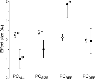
Estimated differences between native and introduced plant populations (i.e. range effect size, or βR) from a statistical model including data from 32 common garden studies of 28 species from 13 flowering plant families. Positive effect sizes indicate larger values in introduced populations relative to native ones, and are estimated for principal components of all measured traits (PCALL), or separate measurements of plant size (PCSIZE), reproduction (PCREP), and defense (PCDEF). We estimated effect sizes by excluding (open circles) or including (closed circles) latitude and range*latitude effects. Approximate standard error bars are shown along with results of significance tests, based on restricted maximum likelihood. Effect sizes that are significantly different from zero (P < 0.05) are indicated with an asterisk.
The inclusion of latitude had a large influence on the estimated difference between native and introduced populations (βR), and on the significance of this difference (Fig. 2). The effect size (βR) of PCALL and PCSIZE reversed and PCSIZE became nonsignificant when latitude was included as a covariate, while PCREP increased 15-fold and became significant (Fig. 2). Thus, for comparisons between native and introduced populations, the significance, magnitude, and direction (i.e. sign) of βR were all highly dependent on latitudinal clines, rendering accurate estimates of the average difference between native and introduced populations impossible.
Statistical testing of individual species not only revealed the presence of latitudinal clines, but also their effects on the significance of βR (i.e. the difference between native and introduced populations). The range-only model revealed a number of significant results, with 42% of models (36 of 86) exhibiting a significant range or range*garden effect. However, 40% of models (31 of 78) also showed significant latitude or latitude*garden effects in the latitude-only model (Appendix B). When both range and latitude were considered in the full model, there was not enough power to detect significant differences between ranges in several species (Appendix B). For example, the number of significant range effects dropped from 36 to 11, while significant latitude effects dropped from 31 to 21 (Appendices B and C). Additionally, 10 of the 11 significant range effects in the full model also showed significant effects of latitude (including interactions with latitude), confirming a strong inter-dependence between range and latitude effects (Appendix C).
To demonstrate more clearly the interdependence of range and latitude evident in Appendices B and C, we chose four species with significant range and latitude effects for the principal component most closely associated with fitness (PCREP). Bivariate plots of phenotype with latitude for these species clearly indicate that range and latitude are confounded, making it difficult to meaningfully compare native and introduced populations, or to accurately estimate the slopes of latitudinal clines (Fig. 3).
Figure 3.
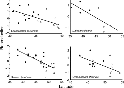
Population means of PCREP (first principal component of reproductive traits) of native (open) and introduced (closed) plant populations plotted against latitude, showing the confounding effects of latitude and range. A single garden from each of four species from Appendix C is shown.
Discussion
Common garden experiments have been used to test EICA and some appear to support rapid evolution during plant invasion (e.g. Blossey and Nötzold 1995; Siemann and Rogers 2001; Leger and Rice 2003; Bossdorf et al. 2004; Genton et al. 2005). However, the results from our analyses reveal that tests of whether introduced genotypes are larger in size or more fecund than native conspecifics are strongly influenced by whether the latitude of populations is explicitly considered in the analysis. We found evidence for latitudinal clines in traits across native and introduced ranges, when all species were considered together (Table 2), and for individual species (Appendices B and C). Because estimated differences between native and introduced populations are highly dependent on the treatment of latitude in statistical models (Fig. 3, Appendix C), this casts doubt on earlier interpretations of the biological basis of trait differences between ranges. Below we discuss these issues in detail and highlight the implications of latitudinal clines in traits for inferences on the ecology and evolution of invasive plants.
Range effects and latitudinal clines
A key issue in invasion biology involves determining the role of rapid adaptive evolution in the establishment and spread of invasive species (Crawley 1987; Reznick and Ghalambor 2001; Sakai et al. 2001; Thébaud and Simberloff 2001; Stockwell et al. 2003; Cox 2004; Lambrinos 2004; Barrett et al. 2008; Keller and Taylor 2008). The EICA hypothesis has stimulated much work in this area because it explicitly predicts that introduced plants should undergo genetically based increases in growth and reproduction, and concurrent declines in physical and chemical defenses. Bossdorf et al. (2005) recently reviewed the results of studies testing EICA and found mixed support for the hypothesis using a vote-counting approach. Our results using quantitative methods revealed significant differences between native and introduced populations for principal components measuring reproduction (PCREP). However, we also found significant effects of range*latitude (i.e. latitudinal clines) for PCREP, PCSIZE, and PCALL (Table 2). Estimated differences between plants from native and introduced ranges were highly contingent on the statistical treatment of these latitudinal clines (Fig. 2).
The estimated difference between native and introduced populations changed substantially, both in magnitude and in direction, when latitude was included in our analyses (Fig. 2). Indeed, in the analysis of 28 species from 32 studies for which latitude was available (Fig. 2), the direction of the difference between native and introduced populations was reversed when latitude was explicitly considered for principal components calculated on all traits (PCALL) and on size (PCSIZE). Hence, in the first case the analysis provided evidence for larger, more robust plants in the introduced range, a key prediction of EICA. However, the inclusion of latitude resulted in a reversal of this effect to larger, more robust plants in the native range, contrary to EICA. In the case of reproduction, a nonsignificant effect became significant and increased 15-fold. Because latitudinal clines in plant traits are common (Appendices B and C), and the effects of range and latitude are strongly inter-related (Fig. 3), any significant difference that is detected in fitness traits between native and introduced ranges should be interpreted cautiously.
Common garden locations
The location of common gardens may also influence estimated differences between native and introduced populations and their biological interpretation. We found a nonsignificant influence of garden when treated as a random effect in our analysis, although some species showed significant garden*latitude, garden*range and garden*range*latitude interactions when analyzed separately as fixed effects (Appendices B and C). This difference can probably be explained because few studies used replicated garden locations (only five of 37 studies in Table 1), and because replication for most species was too low to test for higher-level interactions, such as range*garden*species, latitude*garden*species and latitude*range*species*garden in the combined analysis.
Genetically divergent populations respond differently to garden treatment location, given significant range*garden and latitude*garden interactions of several species (Appendices B and C). As populations are replicated, these results demonstrate genotype-by-environment (GxE) interactions, as demonstrated by Williams et al. (2008). Although the evolutionary significance of GxE interactions is not always considered in studies testing EICA, we found evidence for GxE effects of seed family, population, and range (i.e. native versus introduced) in every study in Table 1 that used more than one common garden location (Willis and Blossey 1999; Siemann and Rogers 2003; Maron et al. 2004a,b; Genton et al. 2005; Widmer et al. 2007; Williams et al. 2008). Similarly, other studies reported significant GxE effects for treatments of herbivory and disease, inter- and intra-specific competition, light, pH, and water availability (e.g., Kaufman and Smouse 2001; Leger and Rice 2003; Bossdorf et al. 2004; DeWalt et al. 2004; Meyer et al. 2005). If population divergence for phenotypic traits is at least partly due to local adaptation, then garden location should favor local genotypes. Therefore, results from investigations based on a single garden location, as occurred in 46 of 54 studies in Table 1, should also be interpreted with extreme caution.
Population structure along environmental gradients
Our results emphasize that variation among populations within a range is more than simple ‘random noise’ that obscures differences between native and introduced conspecifics. Rather, latitudinal clines were common in the combined analysis (Table 2) and for individual species (Appendices B and C). Parallel clines were found when latitude and/or garden*latitude effects were significant but range*latitude or garden*range*latitude interactions were not significant in the (full model) analysis of six species: Eschscholzia californica, Hypericum perforatum, Solidago canadensis, Aegilops cylindrica, Bromus tectorum, and Echinochloa crus-galli. However, we note that results from the last three species involved analyses with <10 degrees of freedom and should therefore be interpreted cautiously (Appendix C). Previous studies have found evidence for clines or other patterns of population divergence in the introduced range paralleling those found in the native range (Weber and Schmid 1998; Huey et al. 2000; Maron et al. 2004b, 2007; Lee et al. 2007; Friedman et al. 2008; Montague et al. 2008). For example, Maron et al. (2004b, 2007) reported evidence for parallel clines in traits associated with growth, reproduction and leaf physiology in European and North American populations of Hypericum perforatum that are unlikely to be associated with introduction history, based on evidence from genetic markers. Collectively, these results suggest that latitudinal clines in plant traits may be more common in introduced species than previously supposed.
Latitudinal clines differing in slope between the native and introduced range of most species were common, given the significant range*latitude effects in our full model (Table 2) and in the analysis of several individual species (Appendix C). Estimates of latitude and range*latitude varied by species. However, any interpretation is complicated by differences in sample size (i.e. the number of populations). The absence of clines in the introduced range cannot explain these interactions, given that the estimated clines in the introduced range were significantly correlated with the native range across all 24 species (Spearman rank R = 0.471, P = 0.020) and were steeper in the introduced range of nine of the 24 species analyzed for PCALL (data not shown). It seems likely that in many cases, different slopes result from local adaptation to environmental factors that differ between the native and introduced range. For example, the same latitudes in North America and Europe will often differ in average temperature, rainfall, and growing season length.
Clines in the native and introduced range of invasive plants offer opportunities to investigate contemporary evolution and the speed of local adaptation. However, latitudinal clines can in principle also be explained by at least two other scenarios. First, other evolutionary processes (i.e. migration and drift) can cause geographical clines that are not necessarily adaptive (Endler 1977). Second, separate introductions from native populations to similar latitudes in the introduced range can result in parallel clines in the absence of selection. Common garden approaches that include careful sampling with respect to environmental gradients, analysis of neutral genetic markers, and reciprocal transplants among different climatic regions, can provide robust methods to test for local adaptation (e.g. Maron et al. 2004b). As yet this integrated approach has not been widely used in comparisons between native and introduced plant populations.
Future recommendations
Our investigation has highlighted several ways of strengthening inferences on adaptive evolution during plant invasion from common garden studies. Most importantly, comparisons of native and introduced populations need sufficient sampling within both the native and introduced range. Limited sample sizes can lead to erroneous estimates of the significance, magnitude, and direction of differences between native and introduced populations, particularly when population differentiation is geographically structured, as it often appears to be. Because significant differences in native and introduced populations can arise from unidentified clines, such geographical variation should be explicitly incorporated into the design and analysis of data from common garden studies. For example, sampling along latitudinal gradients in both the native and introduced range allows the inclusion of latitude as a covariate (e.g. Maron et al. 2004b, 2007). This can be challenging for recently established species and for island invasions because the latitudes occupied by introduced populations may overlap little with the native range. In such cases, incorporation of latitude as a covariate, while excluding range*latitude, will greatly improve statistical models relative to ANOVA (Fig. 3). Direct measurement of abiotic factors, such as season length or growing-degree-days, may also prove useful in cases where latitude does not correlate well with the abiotic environment.
Differences between native and introduced populations will also be contingent on common garden conditions, especially when genotype × environment interactions occur. Because introduced populations may be locally adapted, future studies should employ multiple common gardens, despite the considerable logistical effort that is involved. Where ethical or legal restrictions prevent outdoor gardens, growth chambers can simulate different environmental factors (e.g. day length, temperature), and glasshouses or other enclosures can be replicated across latitudes under ambient conditions. Unfortunately, studies to date have been overly reliant on results from a single common garden location (46 of 54 studies; 37 of 43 species; Table 1) and this may have biased evolutionary inferences.
Integrating neutral genetic markers with common garden studies of quantitative traits may also improve evolutionary inferences concerning the mechanisms responsible for population differentiation (Maron et al. 2004b; Taylor and Keller 2007; Keller and Taylor 2008). Genetic markers have proven particularly useful for identifying the number and location(s) of invasion sources and patterns of spread (e.g. Novak and Mack 1993, 2001; Lee 1999; Neuffer and Hurka 1999; Cristescu et al. 2001; Maron et al. 2004b; Taylor and Keller 2007). Finally, because some data sets are consistent with local adaptation during plant invasion, direct measurements of natural selection on phenotypes (Lande and Arnold 1983; Endler 1986) should help to identify the particular traits under selection during invasion (Maron et al. 2007; Franks et al. 2008). Together these approaches will enable more accurate inferences on the relative importance to plant fitness of stochastic and deterministic forces during the invasion process.
Acknowledgments
We are grateful for the unpublished data generously provided by D. Blumenthal, O. Bossdorf, L. Caño, Y. Chun, M. Cripps, S. DeWalt, A. Erfmeier, S. Franks, S. Güsewell, R. Handley, H. Hull-Sanders, J. Joshi, S. Kaufman, M. van Kleunen, S. Lavergne, E. Leger, G. Meyer, M. Schwarzlaender, T. Widmer, J. Williams and L. Wolfe. We also thank S. Yakimowski, M. Vallejo-Marín, J. Stinchcombe, R. Mack, S. Hill, M. Lajeunesse and two anonymous reviewers for comments on earlier drafts of the manuscript. This research was funded through graduate fellowships to RIC from the Natural Sciences and Engineering Council of Canada, the Ontario Government and the University of Toronto, and through an NSERC Discovery Grant and support from the Canada Research Chair's program to SCHB. JLM was supported by NSF grant DEB-0296175 and DEB-0614406. Collaboration on this work was facilitated by the Global Invasions Network (NSF RCN DEB-0541673).
Supporting Information
Additional Supporting Information may be found in the online version of this article:
Table S1. List of species, traits, and treatment or location of the population means used in our analysis.
Table S2. Proportion of variation in population means explained by principal components for each garden in each study.
Appendix A. Reference list of common garden studies. The ‘Ref #’ column matches the reference number in Table 1.
Appendix B. Results of the ‘range-only’ and ‘latitudeonly’ fixed-effects models for individual species.
Appendix C. Results of the ‘full’ fixed-effects models for individual species.
Please note: Wiley-Blackwell are not responsible for the content or functionality of any supporting materials supplied by the authors. Any queries (other than missing material) should be directed to the corresponding author for the article.
Literature cited
- Abramoff MD, Magelhaes PJ, Ram SJ. Image processing with ImageJ. Biophotonics International. 2004;11:36–42. [Google Scholar]
- Barrett SCH, Colautti RI, Eckert CG. Plant reproductive systems and evolution during biological invasion. Molecular Ecology. 2008;17:373–383. doi: 10.1111/j.1365-294X.2007.03503.x. [DOI] [PubMed] [Google Scholar]
- Blossey B, Nötzold R. Evolution of increased competitive ability in invasive non-indigenous plants: a hypothesis. Journal of Ecology. 1995;83:887–889. [Google Scholar]
- Blows MW, Hoffman AA. A reassessment of genetic limits to evolutionary change. Ecology. 2005;86:1371–1384. [Google Scholar]
- Bossdorf O, Prati D, Auge H, Schmid B. Reduced competitive ability in invasive non-indigenous plants: a hypothesis. Journal of Ecology. 2004;83:887–889. [Google Scholar]
- Bossdorf O, Auge H, Lafuma L, Rogers WE, Siemann E, Prati D. Phenotypic and genetic differentiation between native and introduced plant populations. Oecologia. 2005;144:1–11. doi: 10.1007/s00442-005-0070-z. [DOI] [PubMed] [Google Scholar]
- Bradshaw WE, Holzapfel CM. Genetic response to rapid climate change: it's seasonal timing that matters. Molecular Ecology. 2008;17:157–166. doi: 10.1111/j.1365-294X.2007.03509.x. [DOI] [PubMed] [Google Scholar]
- Connover DO, Schultz ET. Phenotypic similarity and the evolutionary significance of countergradient variation. Trends in Ecology and Evolution. 1995;10:248–252. doi: 10.1016/S0169-5347(00)89081-3. [DOI] [PubMed] [Google Scholar]
- Cox GW. Alien Species and Evolution. Washington: Island Press; 2004. [Google Scholar]
- Crawley MJ. What makes a community invasible? In: Gray AJ, Crawley MJ, Edwards PJ, editors. Colonization, Succession, and Stability. Oxford: Blackwell Scientific; 1987. pp. 429–453. [Google Scholar]
- Cristescu MEA, Hebert PDN, Witt JDS, MacIsaac HJ, Grigorovich IA. An invasion history for Cercopagis pengoi based on mitrochondrial gene sequences. Limnology and Oceanography. 2001;46:224–229. [Google Scholar]
- DeWalt SJ, Denslow JS, Hamrick JL. Biomass allocation, growth and photosynthesis of genotypes from native and introduced ranges of the tropical shrub Clidemia hirta. Oecologia. 2004;138:521–531. doi: 10.1007/s00442-003-1462-6. [DOI] [PubMed] [Google Scholar]
- Endler JA. Geographic Variation, Speciation, and Clines. Princeton: Princeton University Press; 1977. [PubMed] [Google Scholar]
- Endler JA. Natural Selection in the Wild. Princeton: Princeton University Press; 1986. [Google Scholar]
- Franks SJ, Pratt PD, Dray FA, Simms EL. Selection on herbivory resistance and growth rate in an invasive plant. The American Naturalist. 2008;171:678–691. doi: 10.1086/587078. [DOI] [PubMed] [Google Scholar]
- Friedman JH, Roelle JE, Gaskin JF, Pepper AE, Manhart JR. Latitudinal variation in cold hardiness in introduced Tamarix and native Populus. Evolutionary Applications. 2008;1:598–607. doi: 10.1111/j.1752-4571.2008.00044.x. [DOI] [PMC free article] [PubMed] [Google Scholar]
- Genton BJ, Kotanen PM, Cheptou PO, Adolphe C, Shykoff JA. Enemy release but no evolutionary loss of defence in a plant invasion: an inter-continental reciprocal transplant experiment. Oecologia. 2005;146:404–414. doi: 10.1007/s00442-005-0234-x. [DOI] [PubMed] [Google Scholar]
- Grosholz ED, Ruiz GM. Biological invasions drive size increases in marine and estuarine invertebrates. Ecology Letters. 2003;6:705–710. [Google Scholar]
- Gurevitch J, Hedges LV. Statistical issues in ecological meta-analyses. Ecology. 1999;80:1142–1149. [Google Scholar]
- Huey RB, Gilchrist GW, Carlson ML, Berrigan D, Serra L. Rapid evolution of a geographic cline in size in an introduced fly. Science. 2000;287:308–309. doi: 10.1126/science.287.5451.308. [DOI] [PubMed] [Google Scholar]
- Huggett RJ. Fundamentals of Biogeography. 2nd edn. Oxfordshire: Routledge; 2004. [Google Scholar]
- Kaufman SR, Smouse PE. Comparing indigenous and introduced populations of Melaleuca quinquenervia (Cav.) Blake: response of seedlings to water and pH levels. Oecologia. 2001;127:487–494. doi: 10.1007/s004420000621. [DOI] [PubMed] [Google Scholar]
- Keller SR, Taylor DR. History, chance and adaptation during biological invasion: separating stochastic phenotypic evolution from response to selection. Ecology Letters. 2008;11:852–866. doi: 10.1111/j.1461-0248.2008.01188.x. [DOI] [PubMed] [Google Scholar]
- Kollman J, Bañuelos MJ. Latitudinal trends in growth and phenology of the invasive plant Impatiens glandulifera (Balsaminaceae) Diversity and Distributions. 2004;10:377–385. [Google Scholar]
- Lambrinos JG. How interactions between ecology and evolution influence contemporary invasion dynamics. Ecology. 2004;85:2061–2070. [Google Scholar]
- Lande R, Arnold SJ. The measurement of selection on correlated characters. Evolution. 1983;37:1210–1226. doi: 10.1111/j.1558-5646.1983.tb00236.x. [DOI] [PubMed] [Google Scholar]
- Langlet O. Two hundred years genecology. Taxon. 1971;20:653–721. [Google Scholar]
- Lee CE. Rapid and repeated invasions of fresh water by the saltwater copepod Eurytemora affinis. Evolution. 1999;53:1423–1434. doi: 10.1111/j.1558-5646.1999.tb05407.x. [DOI] [PubMed] [Google Scholar]
- Lee CE, Remfert JL, Chang YM. Response to selection and evolvability of invasive populations. Genetica. 2007;129:179–192. doi: 10.1007/s10709-006-9013-9. [DOI] [PubMed] [Google Scholar]
- Leger E, Rice KJ. Invasive California poppies (Eschscholzia californica Cham.) grow larger than native individuals under reduced competition. Ecology Letters. 2003;6:257–264. [Google Scholar]
- Maron JL, Vilà M, Arnason J. Loss of enemy resistance among introduced populations of St. Johns wort (Hypericum perforatum. Ecology. 2004a;85:3243–3253. [Google Scholar]
- Maron JL, Vilà M, Bommarco R, Elmendorf S, Beardsley P. Rapid evolution of an invasive plant. Ecological Monographs. 2004b;74:261–280. [Google Scholar]
- Maron JL, Elmendorf S, Vilà M. Contrasting plant physiological adaptation to climate in the native and introduced range. Evolution. 2007;61:1912–1924. doi: 10.1111/j.1558-5646.2007.00153.x. [DOI] [PubMed] [Google Scholar]
- Meyer G, Clare R, Weber E. An experimental test of the evolution of increased competitive ability hypothesis in goldenrod, Solidago gigantea. Oecologia. 2005;144:299–307. doi: 10.1007/s00442-005-0046-z. [DOI] [PubMed] [Google Scholar]
- Montague JL, Barrett SCH, Eckert CG. Re-establishment of clinal variation in flowering time among introduced populations of purple loosestrife (Lythrum salicaria, Lythraceae) Journal of Evolutionary Biology. 2008;21:234–245. doi: 10.1111/j.1420-9101.2007.01456.x. [DOI] [PubMed] [Google Scholar]
- Müller-Schärer H, Schaffner U, Steinger T. Evolution in invasive plants: implications for biological control. Trends in Ecology and Evolution. 2004;19:417–422. doi: 10.1016/j.tree.2004.05.010. [DOI] [PubMed] [Google Scholar]
- Neuffer B, Hurka H. Colonization history and introduction dynamics of Capsella bursa-pastoris (Brassicaceae) in North America: isozymes and quantitative traits. Molecular Ecology. 1999;8:1667–1681. doi: 10.1046/j.1365-294x.1999.00752.x. [DOI] [PubMed] [Google Scholar]
- Novak SJ, Mack RN. Genetic variation in Bromus tectorum (Poaceae): comparison between native and introduced populations. Heredity. 1993;71:167–176. [Google Scholar]
- Novak SJ, Mack RN. Tracing plant introduction and spread: genetic evidence from Bromus tectorum (Cheatgrass) BioScience. 2001;51:114–122. [Google Scholar]
- Reznick DN, Ghalambor CK. The population ecology of contemporary adaptations: what empirical studies reveal about the conditions that promote adaptive evolution. Genetica. 2001;112:183–198. [PubMed] [Google Scholar]
- Sakai AK, Allendorf FW, Holt JS, Lodge DM, Molofsky J, With KA, Baughman S, et al. The population biology of invasive species. Annual Review of Ecology, Evolution and Systematics. 2001;32:305–332. [Google Scholar]
- Schluter D. Evolution along lines of least resistance. Evolution. 1996;50:1766–1774. doi: 10.1111/j.1558-5646.1996.tb03563.x. [DOI] [PubMed] [Google Scholar]
- Shapiro SS, Wilk MB. An analysis of variance test for normality (complete samples) Biometrika. 1965;52:591–611. [Google Scholar]
- Siemann E, Rogers WE. Genetic differences in growth of an invasive tree species. Ecology Letters. 2001;4:514–518. [Google Scholar]
- Siemann E, Rogers WE. Increased competitive ability of an invasive tree may be limited by an invasive beetle. Ecological Applications. 2003;13:1503–1507. [Google Scholar]
- Stockwell CA, Hendry AP, Kinnison MT. Contemporary evolution meets conservation biology. Trends in Ecology and Evolution. 2003;18:94–101. [Google Scholar]
- Taylor DR, Keller SR. Historical range expansion determines the phylogenetic diversity introduced during contemporary species invasion. Evolution. 2007;61:334–345. doi: 10.1111/j.1558-5646.2007.00037.x. [DOI] [PubMed] [Google Scholar]
- Thébaud C, Simberloff D. Are plants really larger in their introduced ranges? The American Naturalist. 2001;157:231–236. doi: 10.1086/318635. [DOI] [PubMed] [Google Scholar]
- Weber E, Schmid B. Latitudinal population differentiation in two species of Solidago (Asteraceae) introduced into Europe. American Journal of Botany. 1998;85:1110–1121. [PubMed] [Google Scholar]
- Widmer TL, Guermache F, Dolgovskaia MY, Reznik SY. Enhanced growth and seed properties in introduced vs. native populations of yellow starthistle (Centaurea solstitialis. Weed Science. 2007;55:465–473. [Google Scholar]
- Williams JL, Auge H, Maron JL. Different gardens, different results: native and introduced populations exhibit contrasting phenotypes across common gardens. Oecologia. 2008;157:239–248. doi: 10.1007/s00442-008-1075-1. [DOI] [PubMed] [Google Scholar]
- Willis AJ, Blossey B. Benign environments do not explain the increased vigour of non-indigenous plants: a cross-continental transplant experiment. Biocontrol Science and Technology. 1999;9:567–577. [Google Scholar]
Associated Data
This section collects any data citations, data availability statements, or supplementary materials included in this article.