Estimation of effective number of breeders from molecular coancestry of single cohort sample

Abstract

The effective population size, N_e, is an important parameter in population genetics and conservation biology. It is, however, difficult to directly estimate N_e from demographic data in many wild species. Alternatively, the use of genetic data has received much attention in recent years. In the present study, I propose a new method for estimating the effective number of breeders N_eb from a parameter of allele sharing (molecular coancestry) among sampled progeny. The bias and confidence interval of the new estimator are compared with those from a published method, i.e. the heterozygote-excess method, using computer simulation. Two population models are simulated; the noninbred population that consists of noninbred and nonrelated parents and the inbred population that is composed of inbred and related parents. Both methods give essentially unbiased estimates of N_eb when applied to the noninbred population. In the inbred population, the proposed method gives a downward biased estimate, but the confidence interval is remarkably narrowed compared with that in the noninbred population. Estimate from the heterozygote-excess method is nearly unbiased in the inbred population, but suffers from a larger confidence interval. By combining the estimates from the two methods as a harmonic mean, the reliability is remarkably improved.

Introduction

The effective population size, N_e, is one of the most important parameters in population genetics and conservation biology, because this parameter determines both the amount of genetic drift and the rate of inbreeding (Crow and Kimura 1970; Falconer and Mackay 1996). N_e can be estimated from demographic data such as the number of parents and the variance in their progeny number (Caballero 1994). However, the demographic data needed to estimate N_e is often not available in many wild species. As an alternative to estimating N_e from demographic data, methods for estimating N_e from genetic data have been developed (for reviews, see Waples 1991; Schwartz et al. 1999; Beaumont 2003; Leberg 2005; Wang 2005). These methods have different time scales on which N_e is measured. Some of them infer the long-term N_e in the past on an evolutionary time scale, and others estimate the current or short-term N_e (Waples 1991; Wang 2005). For solving practical issues such as managing a small population of endangered species, an accurate estimate of the current or short-tem N_e is of special importance, which is a major concern of this study.

To date, three methods are available for this purpose: the temporal method (Nei and Tajima 1981; Pollak 1983; Waples 1989), the linkage disequilibrium method (Hill 1981) and the heterozygote-excess method (Pudovkin et al. 1996; Luikart and Cornuet 1999). These methods actually assess the effective number of breeders (N_eb) of a cohort from which a sample is obtained. If the sample consists of reproductive adults, N_eb is nearly equivalent to N_e in populations with nonoverlapping generations (Schwartz et al. 1999; and as will be discussed later). N_e can be estimated from N_eb in populations with overlapping generations, if the age structure is known (Waples 1991).

The logic behind the temporal method is that the change of allele frequency in samples separated in time is a reflection of genetic drift. This method is the most tested of the genetic N_eb estimators and has been used to estimate N_eb of various species (Schwartz et al. 1999). The primary weakness of this method is that two or more samples separated in time are necessary (Schwartz et al. 1999). This can be expensive and, by nature, time-consuming. The linkage disequilibrium method is based on the fact that genetic drift generates nonrandom association among alleles in different loci. Despite of the obvious advantage that this method can be used to estimate N_eb from a single cohort sample, there are several drawbacks (Schwartz et al. 1999; Wang 2005). Perhaps, the most critical one is that the estimator assumes an isolated equilibrium population with a constant effective size, which may not be tenable for natural populations of endangered species. The heterozygote-excess method is based on the fact that when the breeding population is small, binomial sampling error produces allele frequency differences between male and female breeders, resulting in an excess of heterozygotes in their progeny (Robertson 1965). As in the linkage disequilibrium method, this method has the advantage that only a single cohort sample is required. Further, this method is appealing because the estimate is easily computed. However, there are few applications of this method, presumably because of the low precision, as empirically shown by Luikart and Cornuet (1999).

Several authors (Waples 1991; Pudovkin et al. 1996; Luikart and Cornuet 1999) emphasized the importance of exploring a method that gives an estimate independent of ones from existing methods, because a combined estimate of several independent estimates is expected to improve the precision of separate estimates. In the present study, a novel method for estimating N_eb from genetic data of a single cohort sample is proposed. The estimator is obtained from a simple parameter (molecular coancestrty) of allele sharing among sampled individuals. Reliability of the new estimator is compared with that from the heterozygote-excess method using computer simulation. Improvement of the reliability attained by combining the two methods is also examined.

Methods

Estimation of N_eb from parent-based coancestry

Although a monoecious diploid population is assumed throughout the following derivation, the extension to dioecious diploid species is straightforward and the same estimation method is applicable to the population.

Let f_t be the coancestry among two randomly sampled individuals in generation t, and P be the probability that two randomly sampled alleles each from different individuals in generation t come from the same individual in generation t − 1. The recurrence equation for the coancestry is given by

1

(Crow and Kimura 1970, p. 102), where F_t−1 is the inbreeding coefficient of individuals in generation t − 1. Following the definition by Crow and Kimura (1970, p. 347), we define the effective number of breeders (N_eb), or strictly the inbreeding effective number, as

2

We set the base population of f_t at the population of generation t − 1 by assuming F_t−1 = f_t−1 = 0. Putting t − 1 = 0 in (1), we obtain from (1) and (2), and

3

This means that an estimate of N_eb can be obtained if the parent-based coancestry (f₁) among individuals in one cohort is estimated.

Estimation of parent-based coancestry

Molecular coancestry

For locus l, molecular coancestry f_M,xy,l (frequently called ‘molecular similarity index’) between individual x having alleles a and b and individual y having alleles c and d is defined as (Malécot 1948)

4

where indicator I_ac is one when allele a of individual x is identical to allele c of individual y, and zero otherwise, etc. When there are L marker loci, molecular coancestry f_M,xy is the average molecular coancestry over all loci (Toro et al. 2002, 2003):

Molecular coancestry will be not only because of alleles that are identical by descent but also because of alleles that are alike in state (AIS). Molecular coancestry is, therefore, an upward biased estimator of the coancestry relative to an arbitrary base population. When s_l denotes the probability that two alleles at locus l are AIS in the base population, the expected molecular coancestry between individual x and y at locus l is (Oliehoek et al. 2006)

5

where f_xy is the coancestry between individuals x and y expressed relative to the base population.

Equation (5) shows that a value for s_l is needed for each locus to obtain f_xy. If allele frequencies in the base population are known without errors, s_l is computed as , where n_l is the number of alleles in locus l and p_i the frequency of ith allele in locus l in the base population. Because allele frequencies in the base population are, however, usually unknown, s_l needs to be estimated. Similar problem is arisen in estimating any relatedness from molecular markers. In most of the published works (e.g. Ritland 1996; Lynch and Ritland 1999), allele frequencies have been estimated from the current population for which relatedness is estimated, meaning that the base population is set equal to the current population. For our purpose, this approximation leads to an apparent contradiction, because it implicitly assumes no drifts in allele frequencies between parent and progeny generations (i.e. N_eb = ∞).

Estimation of f₁from f_M,xy

Irrespective of the upward bias, simulations suggest that molecular coancestry can be a good indicator of the coancestry relative to an arbitrary base population (e.g. Toro et al. 2003; Oliehoek et al. 2006). We take advantage of this property to convert the molecular coancestry to the parent-based coancestry (f₁).

Suppose that n individuals are sampled from progeny in a given generation, for which f₁ is estimated. We assume that the sample consists of at least two nonsib families. This assumption will be satisfied except for a population with an extremely small number of parents, such as a population with only one male parent in polygynous species. Thus, for a given individual in the sample, at least one nonsib pair should be involved in the possible n − 1 pairs with other sampled members. Underlying concept of our estimation is that the nonsib pairs could be inferred from molecular coancestry. Fernández and Toro (2006) showed that a sib-ship can be reconstructed from molecular coancestry with a high accuracy, suggesting that the inference on nonsib pairs based on molecular coancestry has a fairly high precision.

We assume that pairs inferred to be nonsibs (putative nonsibs) are true nonsibs (i.e. f_xy = 0). Thus, substituting the average molecular coancestry () for locus l over all pairs of putative nonsibs into (5) gives an estimate of s_l:

6

With the weight w_l to optimize the contributions of loci to the estimate of coancestry, suggested by Oliehoek et al. (2006), the parent-based coancestry between individuals x and y, f_1,xy, is estimated as

where

(Oliehoek et al. 2006)

and is the estimated frequency of allele i in locus l from the sampled individuals. Note that the weight w_l puts more weight on loci with small s_l and with lots of alleles at nearly equal frequency. The estimate of f₁ is simply obtained by averaging over pairs:

And from (3), N_eb is estimated by

7

Selection method for putative nonsib pairs

The simplest method for selecting putative nonsibs from all the possible pairs is to select a given number (n₀) of pairs with the smallest molecular coancestry. However, this method leads to an underestimation of s_l, because of the positive correlation between f_M,xy and f_M,xy,l due to the finite number of marker loci (L). For example, in an extreme case where only one marker locus is available (L = 1), the selection of the smallest f_M,xy automatically results in the selection of pairs with the smallest f_M,xy,l. When the number of selected pairs (n₀) is much smaller than the number of the actually existing nonsib pairs, the average of f_M,xy,l over the selected n₀ pairs is expected to be lower than that of f_M,xy,l over all the actually existing nonsib pairs, leading to an underestimation of s_l [cf. equation (6)].

In a strictly statistical sense, the selection of putative nonsibs for the estimation of s_l should be based on data independent of the sample from which s_l is estimated. This problem could be largely solved by excluding the information on locus l in selecting putative nonsib pairs for the estimation of s_l. Denoting the molecular coancestry between individuals x and y excluding the information on locus l by f_M,xy,/l, we can compute it as

8

For estimating s_l, the selection of n₀ pairs with the smallest coancestry is based on this partial molecular coancestry.

In the present study, the following selection method was applied: (i) Give the sequential numbers (i = 1, 2, …, n) to n sampled individuals. (ii) For the first individual (i = 1), a pair with the smallest f_M,xy,/l [computed from (8)] is selected from n − 1 pairs with other members. (iii) For the proceeding individual (i ≥ 2), a pair with the smallest f_M,xy,/l is selected in the same manner. But if the pairs already selected in the previous selection are included in n − 1 candidate pairs, the pairs are excluded from the candidates to avoid doubly selecting the same pairs. (iv) As a result, we obtain n₀(=n) pairs with the smallest f_M,xy,/l; (v) averaging f_M,xy,l [computed from (4)] over the n₀ pairs. The average () is the estimate of s_l [cf. equation (6)]. (vi) Steps (ii)–(v) are repeated until estimates of s_l are obtained for all marker loci.

Computer simulation

Computer simulation was carried out to evaluate the reliability of the presented method. Genotypes of individuals in the initial population were generated by assigning alleles randomly sampled from an infinite (conceptual) gene pool with a uniform allele frequency distribution with two alleles for the ‘low-polymorphic’ marker loci case or 10 alleles for the ‘high-polymorphic’ marker loci case. The number of loci was 80 for both polymorphic cases. Prior to progeny sampling for the estimation of N_eb, eight generations of random mating with a breeding system defined below were simulated to accumulate inbreeding and relationship. As the breeding system, monogamy and polygyny were modeled. Under monogamy model, an equal number of male and female parents (N/2) were randomly paired to form N/2 permanent couples. Progeny (parent of the next generation) was produced from a randomly sampled couple, and the sampling of a couple and the reproduction were repeated until N/2 replacements of each sex have been obtained. Under polygyny model, N_m males and N_f (>N_m) females were generated, and each female was mated with a randomly sampled male (thus, there are N_f fixed matings). Progeny was produced from a randomly sampled mating, and this was replicated to obtain N_m males and N_f females for the parents of the next generation. In the final generation, a sample of n progeny was obtained in the same manner of reproduction of the respective breeding system. From the loci each with at least two segregating alleles in the sampled progeny, L = 5–30 loci were randomly chosen as marker loci. For the standard parental population size, N = 10 in monogamy, and N_m = 5 males and N_f = 20 females in polygyny were computed. Sample size of progeny (n) in the final generation was 100 for the two breeding systems. In the low-polymorphic marker loci case, all the marker loci should have exactly two alleles (n_l = 2) as in single nucleotide polymorphisms, but the allele frequency distribution is varied among the loci. In the high-polymorphic marker loci case, not only the allele frequency distribution but also the number of alleles is varied among the loci. In the above standard population size, the average numbers of alleles per marker locus was 3.83 in monogamy, and 5.31 in polygyny, which would be comparable with the allele number of microsatellite markers in a practical survey. This type of data generation is referred to as the ‘inbred population’ model, in a sense that the parental population of sampled progeny consists of inbred and related individuals, which will be a general situation of endangered species populations.

As another type of data generation, the ‘noninbred population’ model was also simulated. The manner for the assignment of initial genotypes and the acceleration of generations were exactly same as in the inbred population, except for that the number of accelerated generations was seven. At the final generation, the allele frequency distribution of each locus was memorized. Then, genotypes of parents were regenerated by assigning alleles randomly sampled from an infinite gene pool with the memorized allele frequency distribution. The sampling of progeny and the choice of marker loci were same as in the inbred population. These procedures could produce a parental population consisting of noninbred and nonrelated individuals but having the same quality of molecular information as in the corresponding inbred population. This type of data generation could be an approximation of a recently recolonized population in an ephemeral habitat.

In additional computations, different sizes of parental population and progeny sample were examined. The effect of unequal contribution of parents on the estimates was also evaluated under monogamy with N = 10, by considering the following two patterns of unequal contributions of N/2 = 5 couples: (0.4, 0.3, 0.1, 0.1, 0.1) and (0.6, 0.1, 0.1, 0.1, 0.1). The number of replicated runs for each combination of population model, breeding system and variables was 5000.

Demographic effective number of breeders (N_eb,demo) under monogamy model was computed from the standard formula of the inbreeding effective size (Caballero 1994):

9

where and are the mean and variance of the number of progeny of couples, respectively. The expression of under the simulated condition is given in Appendix A. N_eb,demo under polygyny is computed as

10

The derivation of this equation is shown in Appendix B. N_eb from pedigree coancestry was also computed, which was simply obtained by substituting the average parent-based pedigree coancestry of sampled progeny into (7). The computed N_eb well agreed with N_eb,demo. Thus, only the value of N_eb,demo was presented in results, and it was referred to as the true value of simulation. In addition to the estimate (denoted as hereafter) obtained from (7), estimate from the heterozygote-excess method (; Pudovkin et al. 1996) was computed for comparison. The locus specific is estimated as

where

and H_obs,i and H_exp,i are the observed and expected proportion of heterozygotes having allele i, respectively. Multiple loci estimate was simply computed as the harmonic mean of over the marker loci, following the previous simulation studies (Pudovkin et al. 1996; Luikart and Cornuet 1999). In both methods, when a negative estimate was obtained, the estimate was regarded as an infinite ().

As a criterion of evaluation, the harmonic mean of estimates over 5000 replicates was computed. Furthermore, to characterize the variation and distribution of estimates, 10th, 50th and 90th percentiles in replicates were calculated. The xth percentile was obtained as the 5000 × (x/100)th smallest estimate in 5000 replicated estimates.

Results and discussion

Left and middle panels in Fig. 1 (A: monogamy and B: polygyny) illustrate the 10th, 50th and 90th percentiles, and a harmonic mean of 5000 replicated estimates of the effective number of breeders (N_eb) from the heterozygote-excess and molecular coancestry methods applied to the noninbred population with L = 5–20 high-polymorphic marker loci. The three percentiles indicate that the distributions of estimates from both methods are skewed upward. The 50th percentile and harmonic mean were, however, close to N_eb,demo (10 for monogamy and 13.79 for polygyny) in both methods. Under monogamy, the interval between 10th and 90th percentiles in tended to be wider than that in , whereas the reversal tendency was observed under polygyny.

Figure 1.

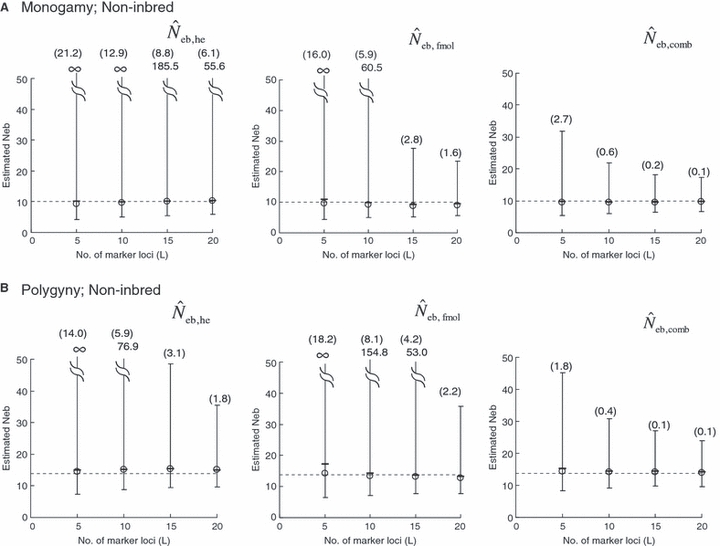
Harmonic mean (marked by open circle), and 10th, 50th and 90th percentiles (marked by bar) of 5000 estimated effective numbers of breeders in the noninbred population under (A) monogamy with N = 10 (half of each sex) parents and (B) polygyny with N_m = 5 male and N_f = 20 female parents, for the case of high-polymorphic marker loci. The sample size of progeny is n = 100. is the estimate from heterozygote-excess method (Pudovkin et al. 1996), the estimate from equation (7) and the estimate by the harmonic mean of and . The value in top of each graph is the clipped 90th percentile, and the value in parentheses is the percentage of replicates with . The dashed line shows the effective number of breeders expected from demographic parameters (N_eb,demo = 10 under monogamy and 13.79 under polygyny, respectively).

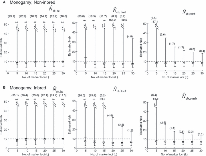
The corresponding simulation results in the inbred population are shown in Fig. 2. Although the 50th percentile and harmonic mean show that the heterozygote-excess method gives an essentially unbiased estimate of N_eb, the estimate from the molecular coancestry method tends to be biased downward. The degree of bias became larger as the number of marker loci increased. Inbreeding and relationship in the parental population gave quite a different impact on the confidence interval in the two methods. The interval between 10th and 90th percentiles in was widened in the inbred population, compared with that in the noninbred population (Fig. 1). The increase of confidence interval was more remarkable under monogamy. In fact, the 90th percentile under monogamy was infinite even with L = 20 marker loci. In contrast, the interval in was remarkably narrowed in the inbred population. For example, the 10th and 90th percentiles in under monogamy with L = 20 marker loci were 3.75 and 12.93, respectively.

Figure 2.

Harmonic mean (marked by open circle), and 10th, 50th and 90th percentiles (marked by bar) of 5000 estimated effective numbers of breeders in the inbred population under (A) monogamy with N = 10 (half of each sex) parents and (B) polygyny with N_m = 5 male and N_f = 20 female parents, for the case of high-polymorphic marker loci. The sample size of progeny is n = 100. is the estimate from heterozygote-excess method (Pudovkin et al. 1996), the estimate from equation (7) and the estimate by harmonic mean of and . The value in top of each graph is the clipped 90th percentile, and the value in parentheses is the percentage of replicates with . The dashed line shows the effective number of breeders expected from demographic parameters (N_eb,demo = 10 under monogamy and 13.79 under polygyny, respectively).

In a strict sense, the heterozygote-excess method is valid only when the progeny are produced by random union gametes (Pudovkin et al. 1996; Luikart and Cornuet 1999). When the progeny are produced by individual-based pairwise matings such as monogamy and polygyny, the sample of progeny is family-structured. In such a sample, heterozygote deficiency generated by the interfamily Wahlund effect may mask the heterozygote excess, reducing the usefulness of the heterozygote-excess method (Luikart and Cornuet 1999). Using computer simulation, Luikart and Cornuet (1999) examined the effect of a family-structured sample on the reliability of the heterozygote-excess method. They found that the heterozygote-excess method gives an essentially unbiased estimate even with a family-structured sample. However, the existence of family structure in sampled progeny substantially increased the variance of estimates under monogamy. Simulation data of Luikart and Cornuet (1999) was generated in the same manner as the noninbred population of the present study. Thus, their sample of progeny contains only sib families. On the other hand, the sample of progeny from the inbred population consists of families with various degrees of relationship (e.g. cousins). The increased confidence interval observed in Fig. 2 indicates that the application of the heterozygote-excess method to such a sample reduces the reliability, although the method still gives an unbiased estimate. The reduction of reliability will be more serious under monogamy (Fig. 2).

As a detail information on the estimation process in the molecular coancestry method, Table 1 gives the observed and estimated [from equation (6)] AIS probability (s_l) in the parental population, and the average estimated parent-based coancestry among actual nonsibs (NS), actual half-sibs (HS), actual full-sibs (FS) and all pairs of sampled progeny, for the case of monogamy and polygyny with L = 15 high-polymorphic marker loci. All the values are shown as the average over 5000 replicates (and over 15 marker loci for s_l). In the noninbred population, the estimated AIS probability was close to the observed value, giving the average estimates of the parent-based coancestries in the three categories (NS, HS and FS) close to the pedigree coancestries, i.e. 0, 0.125 and 0.25 for NS, HS and FS, respectively. Thus, the molecular coancestry method gives an essentially unbiased estimate of N_eb for the noninbred population (Fig. 1). However, the process of selecting putative nonsibs in the molecular coancestry method causes a problem when applied to the inbred population. The selection method may select the actual nonsibs with a reasonably high probability. But the putative nonsibs selected from the inbred population may be less-related nonsibs with regard to further back ancestral relationships than the average nonsibs among the sampled progeny. As seen from Table 1, this causes an underestimation of AIS probability, implying that the base population for coancestry is set at a further back generation over the parental generation. This overrun in setting the base population results in an overestimation of the parent-based coancestry, leading to a downward bias of as observed in Fig. 2. Irrespective of this drawback, the narrow confidence interval of in the inbred population is attractive in its practical use. Although the molecular coancestry method will be less useful for a point estimate of N_eb in inbred populations, it will be useful for detecting a small N_eb.

Table 1.

Observed and estimated AIS probability, and estimated parent-based coancestries among actual nonsibs (NS), actual half-sibs (HS), actual full-sibs (FS) and all pairs of sampled progeny from the noninbred and inbred parental populations under monogamy with N = 10 parents or polygyny with N_m = 5 male and N_f = 20 female parents, for the case of L = 15 high-polymorphic marker loci and the sample size of n = 100.

		AIS probability		Estimated parent-based coancestry among
Breeding system	Population	Observed	Estimated	Actual NS	Actual HS	Actual FS	All pairs
Monogamy	Noninbred	0.3587	0.3571	0.0045	–	0.2552	0.0546
	Inbred	0.3565	0.3366	0.0346	–	0.2651	0.0806
Polygyny	Noninbred	0.2967	0.2972	0.0008	0.1259	0.2503	0.0370
	Inbred	0.2981	0.2830	0.0237	0.1418	0.2592	0.0579

The AIS probability is the average over 5000 replicates and 15 marker loci, and the coancestry is the average over 5000 replicates.

The simulation results for the estimation with the low-polymorphic marker loci are shown in the left and middle panels in Fig. 3(A) for noninbred and Fig. 3(B) for inbred populations in monogamy. Results in polygyny (data not shown) were essentially similar to those in monogamy. As seen from the 10th and 90th percentiles in , the heterozygote-excess method suffers from a larger confidence interval. In fact, even with L = 30 marker loci, the 90th percentile in was still infinite in both noninbred and inbred populations. In contrast, the molecular coancestry method gave an estimate with a practically acceptable confidence interval when L = 30 marker loci were available.

Figure 3.

Harmonic mean (marked by open circle), and 10th, 50th and 90th percentiles (marked by bar) of 5000 estimated effective numbers of breeders in the (A) noninbred and (B) inbred populations under monogamy with N = 10 (half of each sex) parents, for the case of high-polymorphic marker loci. The sample size of progeny is n = 100. is the estimate from heterozygote-excess method (Pudovkin et al. 1996), estimate from equation (7) and the estimate by harmonic mean of and . The value in top of each graph is the clipped 90th percentile, and the value in parentheses is the percentage of replicates with . The dashed line shows the effective number of breeders expected from demographic parameters (N_eb,demo = 10).

Table 2 shows the results from simulation runs with additional combinations of the number of parents and sample size, for the case of L = 15 high-polymorphic marker loci. As the harmonic mean of replicated estimates well agreed with the 50th percentile, it was not shown in the table. The general properties of estimates, e.g. a small bias of estimation from both methods in the noninbred population and a downward bias of in the inbred population, were similar to those observed in Figs 1–3. A remarkable point in Table 2 is a narrower confidence interval of in a small sample of progeny from a small inbred population. For example, under monogamy with N = 10 parents, the 90th percentile of from n = 10 progeny was 38.2, while the corresponding percentile of was infinite. In most of the practical situations of conservation biology, the population in question will be small and inbred, and may suffer from a low reproductive ability. The molecular coancestry method could significantly contribute to the detection of small N_eb of such populations. The magnitude of the downward bias of increased in a larger inbred population, as seen from the 50th percentiles in monogamy with N = 50 and polygyny with N_m = 20 and N_f = 80, which may limit the usefulness of the molecular coancestry method. However, even in these populations, the narrow confidence interval of would be of practical significance for obtaining a conservative estimate of N_eb.

Table 2.

Percentiles (10th, 50th and 90th) of estimated effective number of breeders for 5000 replicated simulation runs in the noninbred and inbred populations with several additional combinations of the number of parents and sample size.

Population and breeding system	N or Nm:Nf	Neb,demo	n	10th	50th	90th	10th	50th	90th	10th	50th	90th
Noninbred
Monogamy	10	10	10	4.84	11.99	∞ (23.2)	4.10	8.27	∞ (10.3)	5.39	9.42	27.01 (2.1)
			20	5.24	11.01	∞ (16.7)	4.48	8.81	114.5 (8.5)	5.90	9.57	24.42 (1.2)
	50	50	50	19.73	55.33	∞ (26.5)	17.0	45.80	∞ (23.1)	22.58	44.75	285.37 (6.3)
Polygyny	5:20	13.79	20	7.63	16.18	∞ (14.4)	6.11	12.42	∞ (12.0)	8.80	13.81	38.51 (1.7)
			50	8.73	15.17	73.97 (5.8)	7.06	13.57	85.49 (6.7)	9.09	14.15	30.01 (0.5)
	20:80	53.78	100	25.28	59.03	∞ (17.6)	21.62	50.24	∞ (18.2)	28.10	52.03	203.54 (3.0)
Inbred
Monogamy	10	10	10	4.46	12.18	∞ (26.5)	3.43	6.70	38.20 (5.7)	4.90	8.03	18.09 (0.9)
			20	4.81	10.99	∞ (22.8)	3.51	6.60	22.29 (3.6)	5.08	7.85	16.58 (0.3)
	50	50	50	17.50	50.37	∞ (23.4)	11.58	20.30	85.59 (4.7)	16.58	27.83	69.50 (1.0)
Polygyny	5:20	13.79	20	7.52	16.19	∞ (17.6)	5.00	9.31	41.06 (4.8)	7.26	11.45	25.37 (0.6)
			50	8.47	15.85	∞ (10.0)	5.31	8.85	21.79 (1.6)	7.71	11.33	19.90 (0)
	20:80	53.78	100	23.61	57.84	∞ (19.7)	15.01	24.62	73.89 (2.6)	21.44	33.73	72.07 (0.4)

Fifteen (L = 15) high-polymorphic marker loci were assumed.

N, the number of parents (half of each sex) in monogamy; N_m, the number of male parents; N_f, the number of female parents in polygyny; N_eb,demo, effective number of breeders expected from demographic parameters; , estimated N_eb from the heterozygote-excess method; , estimated N_eb from equation (7); , harmonic mean of and .

Figures in parentheses are the percentage of replicates with .

The effect of unequal contributions of parents on estimates of N_eb is shown in Table 3, in which a monogamy with N = 10 (half of each sex) and a sample size of n = 100 offspring was assumed. In all the cases computed, the 90th percentile in the molecular coancestry method was much smaller than in the heterozygote-excess method. As unequal contribution of parents is an important factor for a smaller N_e than the census number of breeders (Frankham 1995), the higher accuracy of the present method observed in Table 3 will be a practically appealing point.

Table 3.

Percentiles (10th, 50th and 90th) of estimated effective number of breeders for 5000 replicated simulation runs with unequal contribution of parents under monogamy in the noninbred and inbred populations with N = 10 (half of each sex) parents and the sample size of n = 100.

Contribution	Neb,demo	Population	10th	50th	90th	10th	50th	90th	10th	50th	90th
0.4, 0.3, 0.1, 0.1, 0.1	7.18	Noninbred	4.53	8.14	302.02 (9.3)	3.59	6.91	18.55 (2.1)	4.81	7.31	13.46 (0.2)
		Inbred	4.07	8.30	∞ (16.9)	2.69	5.45	14.09 (1.1)	4.09	6.31	10.95 (0)
0.6, 0.1, 0.1, 0.1, 0.1	5.03	Noninbred	3.80	6.82	107.07 (8.8)	2.26	4.74	13.90 (2.0)	3.40	5.42	9.94 (0.1)
		Inbred	3.63	7.24	∞ (14.6)	1.76	4.17	12.50 (1.6)	2.96	5.02	8.90 (0.1)

Fifteen (L = 15) high-polymorphic marker loci were assumed.

Contribution: expected contributions of =5 couples to sample.

N_eb,demo, effective number of breeders expected from demographic parameters; , estimated N_eb from the heterozygote-excess method; , estimated N_eb from equation (7); , harmonic mean of and .

Figures in parentheses are the percentage of replicates with .

Figure 4 represents the joint distribution of estimates from the heterozygote-excess and molecular coancestry methods applied to the inbred populations under polygyny with N_m = 5 and N_f = 20 parents and L = 15 high-polymorphic marker loci. The moment and Spearman’s rank correlations, excluding the pairs with infinite estimate, were −0.003 and −0.164, respectively. In all other cases simulated, the correlations of these orders were obtained. An interesting point in Fig. 4 is that the incidence of overestimations in the two methods tends to be exclusive. At present, it is not theoretically obvious how to combine several estimates of N_eb optimally to give a single best estimate (Wang 2005). As a tentative method, I combined the two estimates as the harmonic mean, according to the suggestion of Waples (1991):

Figure 4.

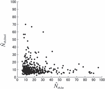
Joint distribution of estimates of effective number of breeders from heterozygote-excess () and molecular coancestry () methods in the inbred population under polygyny with N_m = 5 male and N_f = 20 female parents and n = 100 sample of progeny. Estimates outside the graph were clipped.

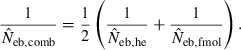The harmonic mean is expected to work well in the present case, because of the exclusive incidence of overestimations in the two methods; an overestimated N_eb returned by one method is filtered out and the combined estimate is largely determined by the estimate from the other method. The property of the combined estimate is shown in the right panels in Figs 1–3 and the column of in Tables 2 and 3. The combined estimate in the inbred population was biased downward because of the downward bias of . However, as expected, the confidence interval of the estimate was substantially narrowed, comparing with the separate estimates. It is notable that the improvement is larger for lower marker quality, i.e. for a smaller number of marker loci and/or a smaller number of alleles in each locus (Figs 1–3), and for a smaller sample size (Table 2). Although the development of an optimal method for combining separate estimates into a single estimate deserves further investigation with sophisticated statistical tools, the above results strongly suggest that a highly reliable estimate can be obtained from the optimal combination.

Some of the limitations of the method proposed in this study are shared by most of the published methods: marker alleles are assumed to be selectively neutral, mating within the population is at random and immigration from other populations is absent (Leberg 2005). In addition, the present method involves a problem associated with age at sampling. Estimation of N_e from the recurrence equation (1) is based on the assumption that the average coancestries in two successive generations are measured as the same age stage. In fact, the application of the present method to a sample of juveniles gives an estimate of ‘the effective number of breeders’. But even in a population with nonoverlapping generations, the estimate can be largely different from N_e, depending on the survival pattern of juveniles to adults. Following Crow and Morton (1955), we consider two extreme patterns of the survival: (i) random survival and (ii) survival of the family as a unit. In the random survival model, survival from juvenile to adult is randomly determined with the expected survival rate s. Under this pattern of survival, the average coancestry among adults is expected to be unchanged from that among the juveniles. Thus, if the present method is applied to a population with nonoverlapping generations, . Under the survival of the family as a unit, the entire juveniles in a family either survive or do not. With the average survival rate s in the population, obtained from a sample of juveniles is related to N_e as (for the theoretical aspect of the above consideration, see Appendix C). Although this model describes an extreme pattern of survival, of animals with low fecundity and high survival rate, such as mammals and birds in which parental nursing for their brood is generally observed, should be cautiously interpreted. On the other hand, will give an appropriate estimate of N_e when the method is applied to animals with high fecundity and low survival rate, such as marine invertebrates and fishes, whose survival seems to be essentially random.

The present method involves additional problems associated with the selection method for putative nonsibs. One is the problem as to the determination of the number (n₀) of selected pairs as putative nonsibs. Although the selection method applied to the present study automatically assigns the number (n) of the sampled progeny to n₀, this is an arbitrary choice. With a smaller n₀, it is more likely that the selected pairs are actually nonsibs, but the coancestry among them will underestimate the AIS probability, and vice versa. Another problem is the drift-induced linkage disequilibrium among marker loci. In small populations, the drift-induced linkage disequilibrium may be an important factor (Hill 1981) and reduce the degree to which loci provide independent information about coancestry. This may reduce the effectiveness of the selection criterion of putative nonsibs defined by equation (8). One potential for solving these problems and improving the estimates of N_eb from molecular coancestry is the use of a sib-ship reconstruction technique. To date, several methods for sib-ship reconstruction from molecular markers have been developed using different algorithms, such as Markov Chain Monte Carlo (MCMC) algorithm (Almudevar and Field 1999; Thomas and Hill 2002; Wang 2004) and simulated annealing (Almudevar 2003; Fernández and Toro 2006), and have been reviewed by Blouin (2003) and Butler et al. (2004). I here take the method proposed by Fernández and Toro (2006) as a trial example of the use of a sib-ship reconstruction technique for estimating N_eb. By the use of their method, we can find the sib-ships among sampled individuals that yield a parent-based coancestry matrix with the highest correlation with the molecular coancestry matrix. A notable feature of their method is that it is free from the assumption of linkage equilibrium among marker loci. Two methods for the use of the reconstructed sib-ships were examined: In the first method (SR1), the reconstructed sib-ships were directly used for computing in equation (7). In the second method (SR2), the average locus-specific coancestry among the inferred nonsib pairs were used for estimating s_l as in equation (6). Simulation with 200 replicates was run for the case of polygyny in the inbred population with N_m = 5 and N_f = 20 parents, n = 100 sample of progeny and L = 15 high-polymorphic marker loci. The results are summarized in Table 4. The two methods with sib-ship reconstruction worked quite well; they gave nearly unbiased estimates and narrower confidence intervals. Although further evaluations including other published methods for sib-ship reconstruction should be carried out under a wide range of scenario, the results in Table 4 suggest the potential for improving the molecular coancestry method.

Table 4.

Harmonic mean and percentiles (10th, 50th and 90th) of two estimates ( and ) of effective number of breeders from 200 replicated simulation runs with a combined use of the molecular coancestry method and a sib-ship reconstruction technique.

		Percentile
Estimate	Harmonic mean	10th	50th	90th
	16.11	9.10	16.41	111.56 (5.5)
	8.07	5.32	8.14	16.33 (0.1)
	14.39	10.74	15.07	18.54 (0)
	12.84	9.66	13.38	17.67 (0)

The corresponding values from the heterozygote-excess () and molecular coancestry () methods are also presented. Polygyny with N_m = 5 male and N_f = 20 female parents in the inbred population with L = 15 high-polymorphic marker loci and the sample size of n = 100 was assumed. The effective number of breeders expected from demographic parameters is 13.79.

Figures in parentheses are the percentage of replicates with .

Appendix A – Expression of in equation (9)

In general, variance of x can be written as

(A1)

where and are the expectation and variance of x conditional on a given y, respectively (Mood et al. 1987, p. 159). We apply this formula to the derivation of expression of .

Let be the expected contribution of ith couple to the cohort of offspring and k_i the number of offspring by ith couple in sample with size n. Applying (A1), we obtain

where is the mean of c_i.

For example, in the simulation condition assumed in Figs 1–3 and Table 2, for all i, giving

Substituting this expression of and into (9) gives

as expected.

Appendix B – Derivation of equation (10)

The effective size (N_e) of populations with unequal sex ratio and variation in mating success has been generally formulated by Nomura (2005). Consider a population of polygynous (harem) breeding system with N_m male and N_f female parents, in which a male mates with several females and a female mates with only one male. Let d_mi be the number of matings of male parent with the mean and variance . Assuming a Poisson distribution of litter size (the number of newborns per mating), the equation given by Nomura (2005) reduces to

(B1)

where is the coefficient of variation of d_mi. Under the condition of the present simulation, the number of matings (d_mi) of male parents follows a binomial distribution with the mean and variance , giving

Substituting this expression into (B1) leads to

Putting N_eb,demo = N_e, we obtain equation (10).

Appendix C – Effect of age at sampling on relation between N_e and N_eb

For simplicity, consider a population of monogamous species with an equal number (N/2 = N_m = N_f) of male and female parents. Generations are assumed to be discrete (nonoverlapping). Let k_ei be the number of offspring at the early age stage (juveniles) contributed by family (couple) i, and k_ai be the number of offspring at the later age stage (reproductive adults) contributed by family i. The average survival rate from juvenile to adult is s. According to the standard formula of effective population size (Caballero 1994), the effective number of breeders of juveniles N_eb and the effective population size N_e (or equivalently the effective number of breeders of adults) are expressed as

and

(C1)

We consider two extreme survival models: (i) random survival and (ii) survival of the family as a unit. Although μ_ka = sμ_ke in both models, the expression of and consequently the relation between N_eb and N_e depend on the model of survival assumed, as shown below.

Random survival

Applying equation (A1) and noting , we obtain an expression of as

(C2)

Substituting (C2) into (C1) gives

Survival of the family as a unit

Under this model, the expression corresponding to (C2) is

Substituting this expression into (C1) leads to

Literature cited

- Almudevar A. A simulated annealing algorithm for maximum likelihood pedigree reconstruction. Theoretical Population Biology. 2003;63:63–75. doi: 10.1016/s0040-5809(02)00048-5. [DOI] [PubMed] [Google Scholar]
- Almudevar A, Field C. Estimation of single-generation sibling relationships based on DNA markers. Journal of Agricultural, Biology, and Environmental Statistics. 1999;4:136–165. [Google Scholar]
- Beaumont MA. Conservation genetics. In: Balding DJ, Bishop M, Cannings C, editors. Handbook of Statistical Genetics. London: Wiley; 2003. pp. 779–812. [Google Scholar]
- Blouin MS. DNA-based methods for pedigree reconstruction and kinship analysis in natural populations. Trends in Ecology and Evolution. 2003;18:503–511. [Google Scholar]
- Butler K, Field C, Herbinger CM, Smith BR. Accuracy, efficiency and robustness of four algorithms allowing full sibship reconstruction from DNA marker data. Molecular Ecology. 2004;13:1589–1600. doi: 10.1111/j.1365-294X.2004.02152.x. [DOI] [PubMed] [Google Scholar]
- Caballero A. Developments in the prediction of effective population size. Heredity. 1994;73:657–679. doi: 10.1038/hdy.1994.174. [DOI] [PubMed] [Google Scholar]
- Crow JF, Kimura M. An Introduction to Population Genetics Theory. Minneapolis: Burgess Publishing; 1970. [Google Scholar]
- Crow JF, Morton NE. Measurement of gene frequency drift in small populations. Evolution. 1955;9:202–214. [Google Scholar]
- Falconer DS, Mackay TFC. Introduction to Quantitative Genetics. 4th edn. Essex: Longman; 1996. [Google Scholar]
- Fernández J, Toro MA. A new method to estimate relatedness from molecular markers. Molecular Ecology. 2006;15:1657–1667. doi: 10.1111/j.1365-294X.2006.02873.x. [DOI] [PubMed] [Google Scholar]
- Frankham R. Effective population size/adult population size ratios in wildlife: a review. Genetical Research. 1995;66:95–106. doi: 10.1017/S0016672308009695. [DOI] [PubMed] [Google Scholar]
- Hill WG. Estimation of effective population size from data on linkage disequilibrium. Genetical Research. 1981;38:209–216. [Google Scholar]
- Leberg P. Genetic approaches for estimating the effective size of populations. The Journal of Wildlife Management. 2005;69:1385–1399. [Google Scholar]
- Luikart G, Cornuet J-M. Estimating the effective number of breeders from heterozygote excess in progeny. Genetics. 1999;151:1211–1216. doi: 10.1093/genetics/151.3.1211. [DOI] [PMC free article] [PubMed] [Google Scholar]
- Lynch M, Ritland K. Estimation of pairwise relatedness with molecular markers. Genetics. 1999;152:1753–1766. doi: 10.1093/genetics/152.4.1753. [DOI] [PMC free article] [PubMed] [Google Scholar]
- Malécot G. Les mathématiques de l’hérédité. Paris: Masson et Cie; 1948. [Google Scholar]
- Mood AM, Graybill FA, Boes DC. Introduction to the Theory of Statistics. 3rd edn. Singapore: McGraw-Hill; 1987. [Google Scholar]
- Nei M, Tajima F. Genetic drift and estimation of effective population size. Genetics. 1981;98:625–640. doi: 10.1093/genetics/98.3.625. [DOI] [PMC free article] [PubMed] [Google Scholar]
- Nomura T. Effective population size under random mating with a finite number of matings. Genetics. 2005;171:1441–1442. doi: 10.1534/genetics.104.029769. [DOI] [PMC free article] [PubMed] [Google Scholar]
- Oliehoek PA, Windig JJ, Van Arendonk JAM, Bijma P. Estimating relatedness between individuals in general populations with a focus on their use in conservation programs. Genetics. 2006;173:483–496. doi: 10.1534/genetics.105.049940. [DOI] [PMC free article] [PubMed] [Google Scholar]
- Pollak E. A new method for estimating the effective population size from allele frequency changes. Genetics. 1983;104:531–548. doi: 10.1093/genetics/104.3.531. [DOI] [PMC free article] [PubMed] [Google Scholar]
- Pudovkin AI, Zaykin DV, Hedgecock D. On the potential for estimating the effective number of breeders from heterozygote-excess in progeny. Genetics. 1996;144:383–387. doi: 10.1093/genetics/144.1.383. [DOI] [PMC free article] [PubMed] [Google Scholar]
- Ritland K. Estimators for pairwise relatedness and individual inbreeding coefficients. Genetical Research. 1996;67:175–186. [Google Scholar]
- Robertson A. The interpretation of genotype ratios in domestic animal populations. Animal Production. 1965;7:319–324. [Google Scholar]
- Schwartz MK, Tallman DA, Luikart G. Review of DNA-based census and effective population size estimators. Animal Conservation. 1999;1:293–299. [Google Scholar]
- Thomas SC, Hill WG. Sibship reconstruction in hierarchical population structure using Markov chain Monte Carlo techniques. Genetical Research. 2002;79:227–234. doi: 10.1017/s0016672302005669. [DOI] [PubMed] [Google Scholar]
- Toro MA, Barragán C, Ovilo C, Rodrigańez J, Rodriguez C, Silió L. Estimation of coancestry in Iberian pigs using molecular markers. Conservation Genetics. 2002;3:309–320. [Google Scholar]
- Toro MA, Barragan C, Ovilo C. Estimation of genetic variability of the founder population in a conservation scheme using microsatellites. Animal Genetics. 2003;34:226–228. doi: 10.1046/j.1365-2052.2003.00988.x. [DOI] [PubMed] [Google Scholar]
- Wang J. Sibship reconstruction from genetic data with typing errors. Genetics. 2004;166:1963–1979. doi: 10.1534/genetics.166.4.1963. [DOI] [PMC free article] [PubMed] [Google Scholar]
- Wang J. Estimation of effective population sizes from data on genetic markers. Philosophical Transactions of the Royal Society B. 2005;360:1395–1409. doi: 10.1098/rstb.2005.1682. [DOI] [PMC free article] [PubMed] [Google Scholar]
- Waples RS. A generalized approach for estimating effective population size from temporal changes in allele frequency. Genetics. 1989;121:379–391. doi: 10.1093/genetics/121.2.379. [DOI] [PMC free article] [PubMed] [Google Scholar]
- Waples RS. Genetic methods for estimating the effective size of cetacean populations. In: Hoelzel AR, editor. Genetic Ecology of Whales and Dolphins, Special Issue 13. London: International Whale Commission; 1991. pp. 279–300. [Google Scholar]