Modeling environmentally associated morphological and genetic variation in a rainforest bird, and its application to conservation prioritization

Abstract

To better understand how environment shapes phenotypic and genetic variation, we explore the relationship between environmental variables across Ecuador and genetic and morphological variation in the wedge-billed woodcreeper (Glyphorynchus spirurus), a common Neotropical rainforest bird species. Generalized dissimilarity models show that variation in amplified fragment length polymorphism markers was strongly associated with environmental variables on both sides of the Andes, but could also partially be explained by geographic distance on the western side of the Andes. Tarsus, wing, tail, and bill lengths and bill depth were well explained by environmental variables on the western side of the Andes, whereas only tarsus length was well explained on the eastern side. Regions that comprise the highest rates of genetic and phenotypic change occur along steep elevation gradients in the Andes. Such environmental gradients are likely to be particularly important for maximizing adaptive diversity to minimize the impacts of climate change. Using a framework for conservation prioritization based on preserving ecological and evolutionary processes, we found little overlap between currently protected areas in Ecuador and regions we predicted to be important in maximizing adaptive variation.

Introduction

There is growing evidence that detailed environmental information is important in understanding variation and diversification in natural populations (e.g. Coyne and Orr 2004; McKinnon et al. 2004; Rundle and Nosil 2005). As more satellite remote-sensing and extrapolated climate surfaces become available, the prospect of investigating genetic and phenotypic divergence at both local and broad habitat scales has become possible (e.g. Scribner et al. 2001; Pilot et al. 2006; Chaves et al. 2007; Smith et al. 2008; Pease et al. 2009). However, few studies have generated detailed maps of biological variation across landscapes using high resolution environmental data, while also taking into account the influence of geographic distance. Doing so is of interest for several reasons. First, the simultaneous analysis of many environmental variables allows one to assess which variables are most important in explaining observed biological variation, and is facilitative in identifying traits that are potentially under selection. Second, taking into account both geographic distance and environmental variation allows one to better understand the factors resulting in diversification. This is particularly important, because environmental variables are generally spatially autocorrelated, and not simultaneously examining the effects of distance and environment can potentially result in incorrect estimates of the environmental component of divergence. Finally, a predictive map of biological variation is useful in developing new experiments for questions regarding modes of diversification and identifying new sampling localities.

Modeling approaches that predict environmentally associated variation also have great potential for application in conservation biology, specifically for the prioritization of areas for future conservation efforts (e.g. Ferrier et al. 2004, 2007). Conservation efforts have long focused on preserving patterns of biodiversity, prioritizing regions to protect based on levels of species richness, endemism, and degree of threat. While such a strategy represents a vital step in prioritizing areas for conservation, it suffers from the limitation that the processes underlying the generation and maintenance of biodiversity are largely ignored (e.g. Frankel 1974; Smith et al. 1993). Recent efforts have begun to focus on conserving both the patterns of biodiversity as well as the evolutionary processes that generate it (Crandall et al. 2000; Cowling and Pressey 2001; Moritz 2002; Mace et al. 2003; Ennos et al. 2005; Smith et al. 2005; Rouget et al. 2006; Bonin et al. 2007; Forest et al. 2007; Davis et al. 2008; Mace and Purvis 2008). Evolutionary processes have typically been incorporated into prioritization efforts using two methods. One employs a measure of evolutionary distinctiveness such as phylogenetic diversity (the branch lengths in a phylogeny) as a surrogate for diversification processes (e.g. Vane-Wright et al. 1991; Faith 1992;Forest et al. 2007). The other relies on detailed knowledge of specific evolutionary processes influencing diversification in given taxa, which is available for few taxonomic groups and few regions of the world (e.g. Cowling and Pressey 2001). Much less attention has been paid to the mechanisms that generate and maintain intra-specific adaptive variation across large geographic areas, yet it is precisely at the intra-specific population level that the study of evolutionary processes is more likely to be fruitful. This dearth of intra-specific studies is due in large part to the near absence of tools to map this variation, or major limitations in their application. Here we integrate newly available climate and remote-sensing variables with existing niche modeling techniques and a recently developed dissimilarity modeling method to map environmentally associated genetic and phenotypic variation in a common rainforest bird species, the wedge-billed woodcreeper (Glyphorynchus spirurus) in Ecuador. Using our results for this species, we demonstrate the utility of a spatially explicit framework for prioritizing areas for conservation. The framework employs recently developed modeling methodologies [species distribution modeling (Phillips et al. 2006) and generalized dissimilarity modeling (GDM; Ferrier et al. 2007)] to map environmentally associated intra-specific variation, as well as traditionally used methods to measure levels of biodiversity.

Study region and focal species

Ecuador is one of the most biotically diverse countries on the planet. It is climatologically and topographically heterogeneous because of the presence of the Andes, with the Amazon basin extending to the east, and the Pacific coastal region to the west (Fig. 1A). As a result of the high altitude and steep slopes of the Andes, climate changes considerably over relatively short distances, resulting in steep environmental gradients. Moreover, the Amazon basin and Pacific coastal regions have their own distinct influences on climatologic conditions on the eastern and western Andean slopes, respectively. Andean species diversity is exceptional, and the region is the only one in the world that is considered a biodiversity hotspot by all three traditionally used measures of biodiversity: species richness, levels of endemism, and degree of threat (Orme et al. 2005). Selection differences caused by diverse ecological and climatic conditions, and isolation resulting from complex topographical features likely resulted in these high levels of biological diversity (e.g. Graham et al. 2004; Chaves et al. 2007). The Andes’ environmental heterogeneity, high levels of biodiversity, and the fact that it is the focus of conservation efforts, make this region an ideal test case to study the effects of environment, barriers, and geographic distance on diversification, and to map biological variation.

Figure 1.

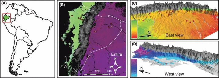
(A) Study region, indicated by the red square, and Ecuador indicated in green; (B–D) predicted patterns of amplified fragment length polymorphism variation for separate generalized dissimilarity modeling analyses on the: (B) entire study area; (C) eastern side of Andes and Amazon lowlands; (D) western side of Andes and lowlands. Regions where wedge-billed woodcreepers do not occur are indicated in black and gray. Pairwise comparison of colors between any two points in the landscape indicates the genetic differentiation between those two points: larger color differences correspond to larger genetic differences (see color bars). Red dots indicate sampling localities. See also Fig. S6.

The wedge-billed woodcreeper is a common and widespread bird species found across lowland tropical regions of South and Central America (Fig. S1) up to about 1500 m in altitude (Ridgely and Greenfield 2001). In Ecuador, populations on either side of the Andes are treated as different subspecies (Glyphorynchus spirurus subrufescens in the west and Glyphorynchus spirurus castelnaudii in the east), belonging to two well-differentiated genetic lineages (Marks et al. 2002; Milá et al. 2009). According to mitochondrial DNA (mtDNA) data, average pairwise divergence between populations across the Andes was 6.98%. Values within each side of the Andes were significant, but much lower (east: 0.41%; west: 0.32%), suggesting ongoing gene flow or recent divergence (Milá et al. 2009). This divergence among populations and the species’ close association with forests across a very heterogeneous region make it a suitable taxon to assess how environmental factors shape biological diversity in tropical forests.

Milá et al. (2009) used genome-wide amplified fragment length polymorphism (AFLP) markers and six fitness-related morphological traits to assess levels of divergence among wedge-billed woodcreeper populations in Ecuador. For the current study, we used this dataset in conjunction with environmental variables from ground stations and satellite-borne sensors that capture climate and habitat characteristics to map the environmentally associated genetic and phenotypic variation continuously across the landscape. In addition, we identified the environmental variables that are important in explaining the variation among populations.

Materials and methods

Molecular markers and morphological data

We used the AFLP dataset from Milá et al. (2009); which consists of 136 loci scored in 178 individuals from 15 sites within Ecuador. Because AFLPs exhibit a relatively high mutation rate, they may be informative for both historical and contemporary processes. For details on the methodology and sampling design, see Appendix and Milá et al. (2009). In brief, whole genomic DNA was digested with restriction enzymes EcoRI and MseI and fragments were ligated to oligonucleotide adapters with T4 DNA ligase. A random sub-sample of fragments was obtained through a pre-selective amplification using primers E-t and M-c, followed by three selective amplifications. Only the selective amplification primer pairs that produced repeatable and unambiguously scorable profiles were used in the analysis. Peaks found in <2% of individuals were excluded. From the binary matrix of allele presence/absence we estimated allelic frequencies using Zhivotovsky's (1999) Bayesian method with uniform prior distributions, and Nei's D genetic distances among sampling sites were then calculated using the method by Lynch and Milligan (1994) as implemented in Genalex 6 (Peakall and Smouse 2006). Nei's D values were subsequently used in GDM (Ferrier et al. 2007; described below) as a measure of population differentiation.

To compare our modeling results to a potential role for historical demography in population divergence, we assessed whether a signal of upslope range expansion since the last glacial maximum (LGM) was present in the genetic data. Haplotype diversity h and nucleotide diversity π for mtDNA was calculated in Arlequin 3.1 (Excoffier et al. 2005), expecting to see lower diversity for populations in areas of range expansion. In addition, as measures of AFLP variation by site we calculated Shannon's Diversity Index I under the assumption of Hardy–Weinberg equilibrium, and the percentage of polymorphic loci in PopGene 3.2 (Yeh et al. 1999), as well as expected heterozygosity in Genalex 6 (Peakall and Smouse 2006).

Morphological variation among wedge-billed woodcreeper populations was assessed through measurement of six fitness-related traits, including (n = 195): wing, tail, tarsus, and bill lengths (defined as exposed culmen, or the length of the bill from tip to the onset where the feathers start); bill width; and bill depth [see Milá et al. (2009) for specific details]. For the current study, we calculated pairwise Euclidean distances from site averages as a measure of dissimilarity between sampling sites, and divided these by the sum of the standard deviations within each site to include within-population variation. We studied the responses of the six variables combined as well of each individual variable. In addition, we assessed the responses of size and shape for the combined set of morphological variables through analyses of principal component scores. Euclidean distances among sites were calculated for PC1 and PC2, and used in GDM analyses.

Environmental data

We compiled a set of moderately high-resolution climate and satellite remote-sensing variables to characterize the sharp habitat transitions in the topographically extremely heterogeneous Ecuadorian Andes (Table S1; Fig. S2). These included bioclimatic variables from the WorldClim database (Hijmans et al. 2005), which are spatially explicit estimates of annual means, seasonal extremes, and degrees of seasonality in temperature and precipitation based on a 50-year climatology (1950–2000), and represent biologically meaningful variables for characterizing species range (Nix 1986).

In addition to these ground-based measurements of climate, we used satellite remote-sensing data from both passive optical sensors (MODIS; http://lpdaac.usgs.gov/lpdaac/products/modis_overview) and active radar scatterometers (QuickScat; http://www.scp.byu.edu/data/Quikscat/SIRv2/qush/World_regions.htm) to infer a broad spectrum of ecological characteristics of the land surface. From the MODIS archive, we used the monthly Leaf Area Index (LAI) to infer vegetation density as well as seasonality (Myneni et al. 2002). In evergreen broadleaf forests, LAI is defined as the one-sided projected green leaf area per unit ground area (Knyazikhin et al. 1998). In addition, we used the vegetation continuous field product (Hansen et al. 2002) as a measure of the percentage of tree cover. From QuickScat (QSCAT), we obtained monthly raw backscatter measurements that capture attributes related to surface moisture and roughness (Long et al. 2001), and from the Shuttle Radar Topography Mission (SRTM), we acquired elevation data.

Time series of the remote-sensing data sources were acquired to roughly match the period of field sampling (QSCAT and treecover from 2001; LAI data represent means over 2000–2004). To improve interpretation, we checked for covariance among variables, and only included those with substantial unique variance. Various criteria were used to decide which layers of correlated pairs were retained for further analysis (with Pearson's correlations on the order of 0.9 or larger). These included maintaining layers that are more commonly used in distribution modeling (WorldClim) or that exhibit larger contrast/variance over the study area (QSCAT) as well as having best data quality (LAI). Variables with native resolutions higher (e.g. SRTM: 30 m) or lower (e.g. QSCAT: 2.25 km) than 1 km were re-aggregated to a 1 km grid cell resolution (Table S1; Buermann et al. 2008).

Measures of distance

Geographic distance between sampling localities can be included in GDM to assess the amount of variation explained by isolation-by-distance (IBD; Wright 1943). As geographic distance per se is not necessarily a good estimate of the distance an individual might travel among localities because of barriers or differences in the permeability of habitats, we included two cost–distance measures, calculated from a cost grid. These were least-cost-paths (LCP; PathMatrix 1.1; Ray 2005) and isolation-by-resistance distances (IBRD, Circuitscape 2.2; McRae 2006) in which unsuitable habitat (defined as those areas predicted to be unsuitable by a species distribution model, after applying a threshold value for suitability; see below) was assumed to be 10 times as difficult to penetrate as suitable habitat. In contrast to LCP, IBRD takes into account the effects of multiple possible pathways with the same cost (McRae 2006). We included water bodies as unsuitable habitat, which seemed justified, because the wedge-billed woodcreeper is a forest bird, and only water bodies of at least 1 km in diameter are detected because of the spatial resolution of the environmental variables. Because the Andes act as a barrier to wedge-billed woodcreepers, and have likely been a barrier since at least the last stage of their uplift, 5 Mya (e.g. Garzione et al. 2008), we also analyzed the effect of the Andes as a barrier by including a layer classifying the west and east as 0 and 1 for analyses across entire Ecuador, which in effect classifies the Andes as impermeable. In addition, we investigated whether other historical barriers besides the Andes may have been present during the LGM. For this purpose, current species distribution was modeled using only temperature and precipitation variables, for which relatively reliable information is available for the LGM. Subsequently, a projection was made on the past by assuming a uniform 6°C decrease in temperature and a 50% decrease in precipitation. These values are within an estimated range based on palaeo-pollen records from Colombia (Van der Hammen and Hooghiemstra 2003), which at these regional scales are likely more accurate than global circulation model reconstructions for the LGM.

Species distribution modeling

Modeling the morphological and genetic variation of the wedge-billed woodcreeper across Ecuador requires delineation of a study area. A map of continuous habitat suitability for this species was generated in a previous study (Buermann et al. 2008), and for the current study we converted it into a presence–absence map using appropriate thresholds (see below). In brief, we used the Maximum Entropy approach implemented in Maxent 3.0 (Phillips et al. 2006), which utilizes presence-only data together with environmental information to estimate the environmental envelop that is suitable for the studied species. Its predictions are continuous logistic probabilities with increasing values referring to more suitable habitats. Maxent performs well with few point localities (Hernandez et al. 2006), and in a recent large model-intercomparison project with 15 other algorithms, Maxent's performance in modeling species’ distributions was generally rated among the highest (Elith et al. 2006). We used 71 localities from a wide area of the wedge-billed woodcreeper's range in Ecuador, Colombia, Peru, and Brazil (Buermann et al. 2008; data available upon request). Our dataset was insufficient to run models for each individual subspecies. However, the wedge-billed woodcreeper appeared to have relatively broad environmental requirements (i.e. presence of humid rainforests). In addition, our prediction of the species’ potential geographic distribution (Fig. S3) was highly consistent with known distributions from bird field guides (Ridgely and Greenfield 2001; Restall et al. 2007), and in agreement with genetic evidence (Marks et al. 2002; Milá et al. 2009) suggesting that the Andes separate the eastern from the western populations. Using the distribution model with pooled locality data to outline areas of suitable habitat as a first step in the analysis seems, therefore, justified.

To convert the continuous Maxent predictions into a presence–absence map defining the study area for subsequent GDM analyses (see below), we used a 10% threshold for habitat suitability, which was centered within the range of a number of optimized Maxent thresholds, including ‘equal training sensitivity and specificity (17%)’ and ‘balance threshold (0.5%)’. Criteria in choosing this threshold level included verification whether the Ecuadorian field sampling sites were included in the suitable area, and comparisons to published range estimates in field guides. Suitable habitat was predicted in some areas above 1500 m in altitude, and because the species does not generally occur above this elevation (Ridgely and Greenfield 2001), we used a conservative maximum altitude of 2000 m a.s.l.

Generalized dissimilarity modeling

To predict the distribution of environmentally associated genetic and phenotypic variation in the wedge-billed woodcreeper across the landscape, we used generalized dissimilarity modeling (GDM; Ferrier et al. 2007). GDM is a matrix regression technique that predicts biotic dissimilarity (turnover) between sites based upon environmental dissimilarity and geographic distance. A major advantage of GDM over other modeling methodologies is that it can fit nonlinear relationships of environmental variables to biological variation through the use of I-spline basis functions (Ferrier et al. 2007). It can explicitly consider the influence of geographic distance on explaining biological variation, and allows for modeling variables that are difficult to define at individual sampling locations, such as genetic markers. It is a two-step method: first, dissimilarities of a set of predictor variables are fitted to the genetic or phenotypic dissimilarities (the response variables). The contributions of predictor variables to explaining the observed response variation are tested by Monte-Carlo permutation, and only those variables that are significant are retained in the final model. These procedures result in a function that describes the relationship between environmental and response variables. Second, using the function resulting from the first step, a spatial prediction is made of the response variable patterns. For visualization purposes, classes of similar response are color coded, where larger color differences between two localities represent larger phenotypic or genetic differences.

Because environmental conditions on opposite sides of the Andes are very different, they may pose different selection regimes upon respective populations. For this reason, and because of a previously observed genetic divergence of populations on either side of the Andes (Milá et al. 2009), we carried out independent analyses on each sub-region, in addition to a broad-scale analysis of the entire region.

To visualize areas harboring the highest amounts of genetic and phenotypic variation, we calculated the standard deviation of 1 × 1 km gridcell values from GDM predictions in an area of 3 × 3 gridcells (equivalent to 3 × 3 km). The center gridcell was assigned the standard deviation value. The resulting map indicates the level of turnover from each gridcell to its neighboring gridcells. We color coded the area comprising the highest 10% standard deviations. In addition, we indicated areas where classes of similar genotypes were present in combination with classes of similar phenotypes. To do this, we used the ‘Combine’ function in ArcGIS 9 on cell values of GDM predictions for genetic and morphological variation. This procedure resulted in a map showing unique combinations of genotype and phenotype. We compared the regions of high turnover with currently protected areas in Ecuador (World Database on Protected Areas; http://www.unep-wcmc.org/wdpa/index.htm) and calculated the amount of overlap as the percentage of gridcells of the highest 10% turnover that are located within currently protected areas.

The relative importance of predictor variables in a GDM can be assessed by means of response curves. Thus, the influence of geographic distance relative to other variables in explaining genetic and phenotypic variation can be assessed. To further evaluate the extent to which geographic distance is potentially correlated with environmental differences, for each region and for each dependent variable we ran independent tests with the following sets of predictor variables: (i) environmental variables and distance (geographic, LCP, or IBRD); (ii) only distance (geographic, LCP, or IBRD); (iii) only environmental variables. Comparison of the results from these three runs provided an indication of the correlation between geographic distance and environmental differences.

To test the robustness of the GDM models, we performed additional model runs in which one or two sites were omitted. The predicted response of the withheld data was plotted against the observed response and compared with the expected line y = x. Furthermore, because no formalized significance testing has yet been developed for GDM, to assess the significance of the level of variation that was explained by our models, we ran additional models in which the environmental layers were substituted by layers with random values for each grid cell. The resulting percentage of variation explained was compared with that of the full model. We considered the performance of the full model not significant if it explained an equal amount or less of the total variation than a model with random environmental variables. Finally, the model outcome and its interpretation may be influenced by the fact that not all environmental space may be sampled. We therefore indicated for each trait, the areas where the values of the most important explanatory variables were outside the range of sampled values (clamping). Particular caution should be taken in interpreting model results in those areas. Because most of the individual variables that were significant in any model contributed relatively little to the full model, we only used the most important variables to assess areas where clamping might occur. We defined the most important variables as those for which response curves reached ≥50% of the maximum response of the single most important variable.

Results

Genetic variation

The full GDM model of AFLP variation across the entire study region (in which all variables were entered simultaneously) explained 95.2% of the total observed variation. It included environmental variables as well as the Andean barrier (Table 1). As expected, the model found the Andes to be a strong barrier to gene flow (Fig. S4). However, models in which only the Andean barrier or only environmental variables were entered performed nearly equally well [93.2% and 90.5% of total variation explained, respectively (Table 1)]. This result suggests that environmental variables are highly divergent between the eastern and western slopes of the Andes, making it unclear whether the differentiation between eastern and western populations is the result of isolation or of environmental differences. With respect to the predicted pattern of the genetic variation, GDM revealed marked divergence between the regions east and west of the Andes, which is consistent with large observed genetic differences across this mountain range. However, GDM did not predict genetic structure within these regions (Fig. 1B).

Table 1.

Generalized dissimilarity modeling results for genetic variation using amplified fragment length polymorphism markers

	Ecuador	W Andes	E Andes
Full model	95.2	98.5	72.2
Significantly contributing variables in full model*	2,7,5,6,9,12,15,16,18	1,4,5,6,7,8,16,18	1,5,6,9,11,12,14,16,17
Using contemporary environment	90.5	98.4	71.5
Using geographic distance	0	50.8	8.8
Using Andean barrier	93.2	–	–
Using random variables	9.1	19.4	28.0

Shown are percentages of total variation explained by models for the entire study region and the regions west and east of the Andes.

^*1 geographic distance; 2 Andean barrier; 3 elevation (SRTM); 4 elevation std (SRTMstd); 5 QSCATMean; 6 QSCATStd; 7 Treecover; 8 LAImax; 9 LAIrange; 10 Bio1; 11 Bio2; 12 Bio4; 13 Bio5; 14 Bio6; 15 Bio12; 16 Bio15; 17 Bio16; 18 Bio17; see Fig. S4 for the relative importance of each variable in the models.

Examining genetic variation west of the Andes, a model for only environmental variables explained 98.4% of the total genetic variation, compared with 50.8% for geographic distance alone and 98.5% for the full model (Table 1). These results indicate that geographic distance was partially correlated with environmental differences. This was further corroborated by plotting geographic distance among sites versus the difference in values for the most important environmental variables (Fig. S5). Precipitation of the driest quarter was the most important variable in explaining the observed variation (Fig. S4), and as a result was the main driver in predicting the genetic variation across the landscape. Because precipitation of the driest quarter changes with elevation along the western slopes of the Andes, the genetic variation also showed a similar elevation gradient (Figs 1D and S6A).

East of the Andes, environmental variables explained a considerable amount of the genetic variation (71.5%), while geographic distance explained little (8.8%), suggesting that habitat differences were more important than IBD in shaping the genetic variation in this region. Genetic variation was predicted to occur along latitudinal and elevation gradients (Figs 1C and S6B). The latitudinal gradient corresponds to variation in precipitation of the wettest quarter and temperature seasonality across the Amazon Basin, whereas the altitudinal gradient along the north-eastern slopes of the Andes was the result of the combined influence of the variables selected by the model (Table 1; Fig. S4). Areas that harbor the highest rates of change are mainly located in the foothills of the Andes (Fig. 3). Only 15.5% of these areas on the western side of the Andes are currently protected, and 8.3% in the east.

Figure 3.

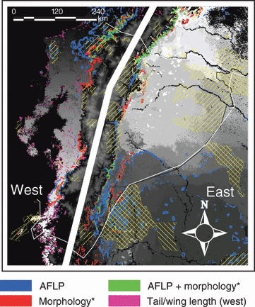
Synthesis of results, showing areas that harbor particularly high levels of turnover of phenotypic and genetic variation (colored regions: area with highest 10% rates of change). The gray scale indicates classes of unique variation that does not occur anywhere else. Because of large population divergence between the west and east of the Andes, colors and gray scales can only be compared within each region. Hatched areas indicate currently protected areas (World Database on Protected Areas). Morphology east of the Andes is represented by tarsus length, and west of the Andes by bill depth. Tail and wing length west of the Andes are indicated separately in green, but show a much diffuser pattern because of the importance of treecover in explaining the variation, and the high level of disturbance in that area. Areas where model confidence was low because they fell outside the environmental space sampled were omitted from this map.

Replacement of geographic distance with LCP or resistance distances that were based on current barriers did not influence models either on the east or the west side of the Andes. In addition, a Maxent model of habitat suitability during the LGM predicted a shift of suitable habitat of ∼400 m downward in altitude along the Andean slopes, and loss of habitat in southwestern Ecuador, but no barriers in addition to those currently existing. Extant populations at higher elevations may be in areas of range expansion since the LGM. Indeed, some sampled populations are within the predicted area of range expansion (Fig. S7), but AFLP and mtDNA diversity indices within populations did not show a pattern with respect to elevation (Table S2; Milá et al. 2009; R² < 0.02, P > 0.5).

Morphological variation

Models for the combined response of all morphological variables (tarsus, tail, wing, and bill length, bill depth and width) explained 73.4% of the variation west, and 42.0% east of the Andes. Because potential selection pressures may act differentially on different morphological traits, we also analyzed morphological variables individually. Variation in four traits (tarsus, wing and tail length, and bill depth) was well explained by environmental variables on both the western and eastern side of the Andes (Table 2). As was the case for genetic variation, the highest rates of morphological change across the landscape can be found along the slopes of the Andes (Figs 2 and 3).

Table 2.

Generalized dissimilarity modeling results for morphological characters

	West of Andes	East of Andes
Tarsus length	*60.7(1,6,8)/0/60.7/34.3	*70.5(4,5,6,9,14)/10.9/70.5/13.8
Wing length	*91.7(6,7,13,14)/6.1/ 91.7/34.3	22.0/–/–/57.1
Tail length	*82.4(1,3,7,9,13)/6.1/81.5/24.6	48.2/–/–/48.7
Bill width	59.2/–/–/61.7	23.7/–/–/42.7
Bill depth	*92.5(1,5,8,9,11,12)/22.7/91.5/11.4	*27.2(1,5,8,9,16,17)/10.4/23.1/2.4
Bill length	*63.9(4,5,6,8,14)/0/63.9/0	18.9/–/–/51.0
All traits combined	*73.4(5,8,10,11)/0/73.4/11.0	*42.0(1,5,7,9,11,16,18)/14.3/41.9/8.9
Size (PC1; 32.1% of total variation)	*81.3(3,7,10)/0/81.3/18.0	9.4/–/–/51.4
Shape (PC2; 25.3% of total variation)	*93.2(1,3,5,6,7,9,13,14,15)/17.3/92.6/14.1	19.3/–/–/42.8

Shown are the percentages of total variance explained by models for the regions west and east of the Andes. For cases in which the full model (using both geographic distance and environment) explained more of the total variation than random models (indicated by ‘^*’), the variables selected by the model are shown in parentheses (see Table 1 for coding of environmental variables), and figures are also shown for models in which only geographic distance or only environmental variables were entered (full model/using distance/using environment/using random environmental variables). See Fig. S4 for the relative importance of each variable in the models.

Figure 2.

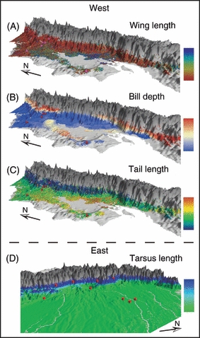
Predicted patterns of morphological variation in the wedge-billed woodcreeper for separate generalized dissimilarity modeling analyses of: (A) wing length; (B) bill depth; (C) tail length; (D) tarsus length. Gray indicates areas where the species is not present. Pairwise comparisons of colors between any two sites in the landscape indicate morphological differences, where large color differences (see bars) represent large morphological differences. Blue (A) and red (B–D) dots indicate sampling localities. See also Fig. S8.

Tarsus length on the eastern side of the Andes was mainly explained by minimum temperature of the coldest month and annual mean QSCAT (Fig. S4), which captures canopy properties related to moisture and roughness (the full model explained 70.5% of total variation). Gradients in these variables along the Andean flanks relate to habitat transitions from the Amazon lowlands to the Andean foothills (Figs 2D and S8D). A linear regression revealed that tarsus length increases with increasing surface moisture levels (R² = 0.73, P < 0.01; Fig. S9). We hypothesize that this correlation is the result of the greater presence of moss covering tree trunks in the moister forests of the Andean foothills. In this environment, longer tarsi may increase the climbing performance and thus the foraging efficiency of individuals, although additional field data will be necessary to properly test this hypothesis (Milá et al. 2009).

Variation in both wing (Figs 2A and S8A) and tail lengths (Figs 2C and S8C) was well explained on the west side of the Andes (91.7% and 82.4%, respectively), and treecover was most influential in this association. Wing length has been shown to be related to treecover in other species as well (e.g. Smith et al. 2008). The predicted variation of wing and tail length showed a fragmented pattern in the central lowlands on the western side of the Andes and a moderately strong gradient associated with elevation.

Finally, variation in bill depth (92.5% explained) showed high turnover along the north- and south-western slopes of the Andes (Figs 2B and S8B), but not along the central-western slopes. This pattern of variation was consistent with the patterns of mean diurnal temperature range and temperature seasonality, which were the most important variables in explaining bill depth variation (Table 2; Fig. S4).

A principle component analysis on the combined morphological variables extracted two principal components (PC). PC1 explained 32.1% of the variation and mainly represented size. PC2 explained 25.3% and mainly represented shape differences. Analyses on the separate responses of size (PC1 scores) and shape (PC2 scores) indicated that the morphological responses in the west are both shape and size related (93.15% and 81.34% of variation explained, respectively; Table 2). However, neither shape nor size responses were well explained in the east (Table 2).

Usage of LCP or resistance distances rather than geographic distance did not influence any of the models for morphological variation, either on the east or the west of the Andes.

On the western side of the Andes, only 7.3% (tail length), 8.9% (wing length), and 16.8% (bill depth) of the areas harboring the highest 10% of turnover overlapped with currently protected areas, and on the eastern side 11.5% (tarsus length).

Model performance

Sensitivity analyses using jackknife procedures suggested overall robustness of the models, even though models for tarsus length on the eastern side of the Andes were less accurate, with slight overpredictions at small observed response values, and underpredictions at higher observed response values (Fig. S10). These results suggest that the observed relation between environmental and genetic or morphological dissimilarities is consistent, and not the chance result of a specific set of sampling sites. With respect to analyses of genetic variation across the entire region, however, models could not distinguish between the relative effects of environment versus the Andes as a barrier: separate models using either environmental variables or the Andean barrier both explained >90% of the total variation (Table 1). In addition, using jackknifing procedures, the larger genetic differences across the Andes were less accurately predicted (Fig. S11) than those within regions. This pattern is inherent to situations where environmental differences highly correlate with the presence of a barrier or geographic distance, and can be dealt with by sampling not only along an environmental gradient, but also among equally spaced populations with the same environmental conditions. Nevertheless, a predictive map of genetic variation across Ecuador suggested a major difference between populations inhabiting areas west and east of the Andes (Fig. 1B), which is consistent with known population structure (Marks et al. 2002; Milá et al. 2009).

Discussion

The topographic heterogeneity of the Andes has resulted in a wide variety of habitats and barriers that are nearly or completely impassable to individuals of many species. Consequently, a combination of vicariant and selective mechanisms has likely resulted in the biological diversity currently observed. Identifying the nature of these evolutionary processes and understanding their effect on the spatial distribution of biodiversity requires simultaneous spatial analyses of the relationship of environmental variables and geographic distance with intra-specific biological variation across the landscape. Such a procedure can facilitate in understanding the relative importance of environment versus distance in shaping biodiversity, in identifying adaptive traits, and in prioritizing areas for conservation. Here we used a comprehensive approach, integrating recently developed spatial analysis tools to map environmentally associated variation in the wedge-billed woodcreeper.

Models of biological variation across the landscape

Past schemes for defining areas of high conservation importance have focused on the species level and identified biodiversity hotspots where species richness or phylogenetic diversity is high (e.g. Vane-Wright et al. 1991; Faith 1992; Orme et al. 2005). An equivalent metric for population level process is only now emerging and initial efforts have emphasized evolutionary history and the preservation of the genetic legacy of a species (Crandall et al. 2000; Cowling and Pressey 2001; Moritz 2002; Mace et al. 2003; Ennos et al. 2005; Smith et al. 2005; Rouget et al. 2006; Bonin et al. 2007; Forest et al. 2007; Davis et al. 2008; Mace and Purvis 2008). For example, recently Carnaval et al. (2009) identified a largely unknown Pleistocene refuge in the Atlantic rainforest of Brazil through analysis of concordant phylogeographic partitions in rainforest frogs. However, such areas may not be those where adaptive diversity is maximal (e.g. Moritz 2002), and thus emphasize history over the potential for response to environmental change at the population level (e.g. Crandall et al. 2000). Further, a phylogeographic approach will miss very recent episodes of local adaptation and genetic isolation where sufficient time has not elapsed such that mtDNA sequence trees show distinct genetic partitions (Pease et al. 2009).

In contrast, our spatially explicit models focus on the relationship between environmental heterogeneity and genetic and phenotypic variation, and emphasize local adaptation and genetic turnover on more recent timescales. Our models generally performed well in explaining genetic and morphological variation (Tables 1 and 2), and suggested a close association between biological and environmental variation. In particular, when regions east and west of the Andes were analyzed separately, environmental variables explained most of the genetic variation, whereas geographic distance explained little, except for genetic variation west of the Andes. Substitution of geographic distance with LCP or resistance distances, which take into account potential levels of connectivity between populations, did not influence model performance. This result could be due to the relatively homogeneous habitat suitability for the species within each region. The fact that geographic distance generally explained little of the genetic and phenotypic variation (or in the case of genetic variation west of the Andes much less than environmental variables), while environmental variables explained a large fraction, suggests that neutral processes because of isolation by distance were relatively less important and that these traits were more likely shaped by natural selection. This suggestion is most likely true for the phenotypic traits that we studied, because these traits have been shown to be fitness related in other species (e.g. Bardwell et al. 2001; Jensen et al. 2004; Milá et al. 2008b). However, because it is unknown to what extent AFLP loci are linked to genes under selection, the close association between genetic and environmental variation may be the combined result of direct selective forces on linked genes and of decreased gene flow because of reduced dispersal ability as a result of habitat differences. Any bias that might occur by using a putatively neutral marker would likely be in the direction of finding larger proportions of variation explained by IBD. However, we find that most of the variation is explained by environmental differences. While the mechanism underlying this result is unclear, it does suggest that environmental differences influence genetic differentiation, and that putatively neutral divergence explained by environmental heterogeneity, but not by IBD, may be a proxy for adaptive differentiation.

An alternative explanation for our finding that environmental heterogeneity was much more important in explaining biological variation than IBD is that historical demographic processes could have potentially interfered with IBD. Range expansions are likely to occur along environmental gradients in a direction where habitat gradually becomes suitable over a period of climate change. For wedge-billed woodcreepers in the Andes, the most likely direction of range expansion since the LGM is from lower to higher altitudes (Fig. S7). However, we did not detect comparatively lower levels of genetic diversity in high-altitude populations, suggesting that if demographic processes were important, we are unable to detect it.

It is noteworthy that both the genetic and the combined morphological patterns of variation were explained by different variables on the east side of the Andes as compared with the west (Tables 1 and 2; Fig. S4), which suggests that different processes may play a role in shaping this variation. Specifically, in the case of genetic variation, three temperature variables were significant on the eastern side of the Andes, whereas on the western side temperature was not significant at all (Table 1). Likewise, for the combined morphological variables, two precipitation variables were significant in the east, whereas no precipitation variables were selected in the west. These differences may be explained by the fact that both climate and remote-sensing variables west of the Andes are much more heterogeneous than those in the east.

Our results suggest that environmental gradients along the slopes of the Andes are a major driver of diversification in wedge-billed woodcreepers. Climate variables were often most influential in explaining the observed biotic variation, yet in some cases remote-sensing variables pertaining to vegetation density or moisture levels were also very important (Tables 1 and 2; Fig. S4). These environmental gradients are mainly related to elevation differences because local climate conditions are largely determined by altitude. As environmental gradients are steepest along the slopes of the Andes, this is where the highest rates of biological change in woodcreepers occurred (Figs 1–3).

Jackknifing procedures indicated that our models performed well in predicting genetic and morphological variation, and were robust to omission of data given the localities that have been sampled. However, some caution should be used in the interpretation of the maps resulting from our models. In areas that are sparsely sampled – such as the southeastern region for the wedge-billed woodcreeper – the corresponding predictions may not be as robust as in areas with more dense sampling regimes. In particular, when the environmental conditions of those areas are outside the range spanned by the sampling sites (we indicated those areas in the maps in the Supporting information), the model extrapolates the genetic and phenotypic response curves. Such extrapolation could potentially result in inaccurate predictions, or at least lower levels of confidence in predicted variation in those areas.

Mapping adaptive variation for conservation prioritization

Recent advances in modeling methodologies and the accessibility of high-resolution interpolated climate and satellite-based ecological data have resulted in new opportunities for the accurate assessment of biodiversity patterns across large geographic areas. We exploited these new developments to map variation in the wedge-billed woodcreeper. To more fully integrate information on biodiversity patterns, processes, and socio-economic factors, we suggest the following multi-step approach, which may be generally applicable for conservation prioritization (Fig. 4).

Figure 4.

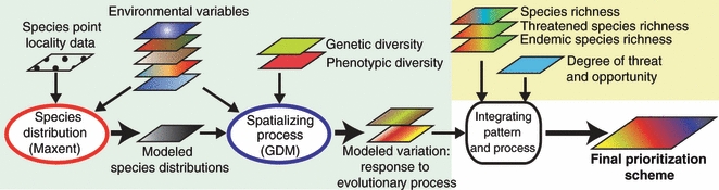
Proposed framework for integrating evolutionary processes (blue box) with traditionally used information on biodiversity patterns, levels of threat, and socio-economic information (yellow box) in conservation planning. Predictive models for spatializing species distributions and environmentally associated genetic and phenotypic variation are at the core of the approach. Modeled species distributions are used to delimit the study area for subsequent modeling of intra-specific variation, and can also provide the basis for the assessment of species richness. Environmental variables are used in modeling both species distributions and intra-specific variation, and could include remotely sensed data (e.g. tree cover, elevation, or moisture levels) and ground-based data (e.g. temperature and precipitation variables). Small arrows represent input, large arrows output.

1 Modeling species distribution

To map intra-specific variation, it is important to first identify the species’ range, because predictions into areas where the species does not occur would provide false information on levels of variation. To estimate a species’ potential geographic distribution, we utilized ecological niche modeling, which has been applied extensively in ecology, evolution, and conservation biology (Guisan and Zimmermann 2000; Rice et al. 2003; Graham et al. 2004; Carstens and Richards 2007; Kozak et al. 2008; Swenson 2008).

2 Mapping intra-specific variation across the landscape

The key step in incorporating evolutionary processes in conservation prioritization is to project environmentally associated biological variation across large areas that have not been sampled, for which we employed GDM (Ferrier et al. 2007). The graphical output of this method is particularly facilitative in visualizing the spatial patterns of variation across a geographic landscape. Because demographic history may also influence patterns of differentiation, it is useful to test for a signal of historical demographic processes in the genetic data.

3 Combining process with pattern and socio-economic factors

Finally, to maximize the information content for prioritizing areas, information on the patterns of biodiversity (e.g. Orme et al. 2005) needs to be incorporated with information on the processes that generate and sustain it, as well as levels of threat (Butchart et al. 2005) and socio-economic factors (e.g. Naidoo et al. 2006;McBride et al. 2007; Wilson et al. 2007). Often, detailed socio-economic information may be scarce, which can hamper the implementation of conservation action (e.g. Knight et al. 2006). Yet, with the availability of global remote-sensing variables, it may often be possible to include some measure of socio-economic data into prioritization (e.g. Sarkar et al. 2004; Cameron et al. 2008).

A worked example: priority areas for conservation in the wedge-billed woodcreeper

The species distribution model developed in the first step of our framework indicated that the wedge-billed woodcreeper is widely distributed across lowland and mid-elevation areas, and is consistent with expert knowledge on the species’ distribution. If one would not take into account intra-specific variation, currently protected areas (World Database on Protected Areas; http://www.unep-wcmc.org/wdpa/index.htm) appear to be sufficient for the wedge-billed woodcreeper, because they overlap with a fairly large area of its distribution (Fig. 3).

Interestingly however, results from the second step, in which we mapped environmentally associated variation, do not support this view. To visualize areas that harbor high levels of variation, we mapped the highest 10% in genetic and phenotypic turnover per unit area (Fig. 3). The highest rates of change are mainly located along the Andean slopes. A likely explanation for this observation is that many of the climatic and remotely sensed environmental variables change with elevation, which results in strong environmental gradients in areas where elevation gradients are steepest. Such gradients are likely to be particularly important for conservation, because in response to climate change, populations will need to either adapt to the new environmental conditions, or shift their ranges to areas where ecological conditions are more favorable (e.g. Hickling et al. 2006; Moritz et al. 2008). Conservation of environmental gradients that harbor high levels of environmentally associated variation could both maximize adaptive variation and allow for gradual range shifts (Smith et al. 2001). Comparisons of the regions that harbor the highest 10% of turnover with the World Database on Protected Areas (http://www.unep-wcmc.org/wdpa/index.htm) revealed that from only 7.3% (tail length on the west) to 16.8% (bill depth on the west) of these areas is currently protected. This result suggests that current levels of protection may not be sufficiently adequate for conservation of process. This insufficient current level of protection is consistent with findings of Sierra et al. (2002) based on analyses of the level of protection of different ecosystems. However, areas that were assigned high priority by Sierra et al. (2002) are not fully consistent with those where we found high levels of turnover in the wedge-billed woodcreeper. This result stresses the importance of mapping intra-specific variation for a multitude of species in this region.

Finally, we primarily focused our analyses on the inclusion of evolutionary processes into conservation assessments because processes such as local adaptation have received relatively little attention in comparison with patterns of species or phylogenetic diversity in conservation prioritization. Yet, we will briefly discuss some of the issues that are of particular importance for Ecuador in the third step of our proposed framework. The Andes are one of the most diverse regions in the world, and traditionally seen as a hotspot for species richness, levels of endemism, and degree of threat (e.g. Sierra et al. 2002; Orme et al. 2005). The region is under great threat by human activity, yet only about a quarter of the remaining 25% area of mature forest is currently protected (Myers et al. 2000). Species losses in the Tropical Andes are predicted to be exceptionally high if habitat destruction does not decrease (Brooks et al. 2002). In addition, climate change may have a large impact on the Andes, because impacts in the tropics are predicted to be largest at higher elevations (Bradley et al. 2004), and palaeo-climatic data suggest that Andean biomes are particularly sensitive to changing conditions (Bush 2002; Van der Hammen and Hooghiemstra 2003). The regions that we identified as important for conservation based on the highest rates of change coincide with relatively less densely populated areas on the eastern side of the Andes (GPW version 3, Gridded Population of the World; http://sedac.ciesin.columbia.edu/gpw/index.jsp; Fig. S12), suggesting an opportunity for conservation limited by relatively modest conflict with human needs. On the western side of the Andes, however, human population densities are higher, which could potentially lead to conflict with conservation strategies (Fig. S12).

To complete the prioritization process, more detailed analyses of the above mentioned types of information are needed. Software packages such as Marxan (Ball and Possingham 2000; Possingham et al. 2000), Target (Faith 1998), and Zonation (Moilanen 2007) can incorporate both biological and socio-economic data to prioritize areas for conservation. Inclusion of information on the levels of variation such as we have shown here would help ensure that evolutionary processes are taken into consideration in conservation planning.

While the wedge-billed woodcreeper is not currently threatened, our study was intended to illustrate how environmentally associated variation can be mapped and incorporated into conservation assessments. We believe the framework for prioritization presented here is advantageous over more traditional approaches that only focus on the patterns of biodiversity, because such approaches may not capture intra-specific adaptive variation, which is likely to be important for species’ ability to persist during climate change. In addition, approaches that focus on surrogates of biodiversity such as species richness will miss recent local adaptation and isolation, where divergence has not progressed sufficiently far for new species to evolve. The approach presented here focused on the relation of environment with intra-specific variation and thus emphasizes local adaptation over a potentially long timeframe, including those that occurred more recently. Ultimately, the full application of this approach will require combining similar data for a host of target species and incorporating predicted shifts resulting from climate change. With advances in analytical techniques and genetic approaches, we believe that integrating such data for a multitude of species is fully achievable.

Appendix

Sampling design

Sampling localities, with sample sizes in brackets, were as follows: Bilsa [13] (N 0.360766 W 79.714866, 650 m), Cumandá [10] (S 1 28.612 W 78 08.595, 1323 m), Pachijal [5] (N 00.18166 W 78.93117, 650 m), Hollín [21] (S 00.68896 W 77.72658, 1200 m), Jatun Sacha [4] (S 01.07215 W 77.62144, 400 m), Loma Alta [7] (S 01.83475 W 80.611433, 610 m), Maldonado [10] (N 00.13453 W 7914402, 405 m), Miazal [5] (S 02.63573 W 77.79831, 300 m), Mindo [16] (S 00.06496 W 78.79338, 1398 m), Bancos [4] (N 00.06479 W 78.98241, 750 m), Pañacocha [21] (S 00.38238 W 76.17612, 400 m), San Rafael [6] (S 00.10082 W 77.58398, 1300 m), Sangay [24](S 02.09883 W 78.15164, 1375 m), Tiputini [19] (S 00.63698 W 76.14912, 400 m), Yasuni [13] (S 00.67455 W 76.39837, 400 m). Sampling localities west and east of the Andes spanned a similar altitudinal range.

AFLP profiling and analysis

Amplified fragment length polymorphism profiles were generated using a protocol modified slightly from Vos et al. (1995). Whole genomic DNA was digested with restriction enzymes EcoRI and MseI and fragments were ligated to oligonucleotide adapters with T4 DNA ligase. A random sub-sample of fragments was obtained through a pre-selective amplification using primers E-t and M-c, followed by three selective amplifications using primer pairs E-tag/M-cga, E-tgc/M-cga, and E-tgc/M-cgt, with each E primer fluorescently labeled with 6FAM dye. Twelve pairs of selective amplification primers were tried, but only the pairs producing repeatable and unambiguously scorable profiles were used in the analysis. Selectively amplified fragments were run in an ABI 3700 genetic analyzer with a LIZ500 size standard. Peaks were visualized using genemapper 3.7 and scored manually, with individuals and populations randomized to avoid observer bias. Only unambiguously scorable loci and individuals were included in the analysis and peaks found in less than 2% of individuals were excluded. Methodological error rate was assessed by running a subset of 10 individuals twice from the pre-selective amplification step. The average per-locus error rate for the AFLP data, measured as recommended by Bonin et al. (2004), was 1.8%, a rate comparable to that of other AFLP studies in birds (Milá et al. 2008a; Smith et al. 2008).

Supporting Information

Additional Supporting Information may be found in the online version of this article:

Figure S1. Distribution of the wedge-billed woodcreeper, Glyphorynchus spirurus, in South America.

Figure S2. Environmental layers used in species distribution models and GDM.

Figure S3. Predicted geographic distribution of the wedge-billed woodcreeper using Maxent (Phillips et al. 2006) and 71 presence localities across the species' range.

Figure S4. Response curves for variables significantly contributing to explaining genetic or morphological variation in the wedge-billed woodcreeper in Ecuador.

Figure S5. Plots of geographic distance between sampling sites versus the two most important environmental variables in explaining AFLP variation on the western side of the Andes, showing a correlation between geographic distance and environmental differences.

Figure S6. Predicted patterns of AFLP variation for independent GDM analysis of: (A) the region west of the Andes; and (B) the region east of the Andes.

Figure S7. Differences in wedge-billed woodcreeper ranges between predictions for the last glacial maximum and current distributions.

Figure S8. Predicted patterns of morphological variation for independent GDM analysis of: (A) wing length; (B) bill depth; (C) tail length; (D) tarsus length.

Figure S9. Correlation between QSCAT mean (mean surface moisture or canopy roughness) and mean tarsus length on the eastern side of the Andes.

Figure S10. Observed versus predicted response in morphological variation between sampling localities, indicating model performance.

Figure S11. Observed versus predicted response in genetic variation (AFLP markers) between sampling localities, indicating model performance.

Figure S12. Priority areas for conservation based on the highest rates of turnover (colors; see Fig. 3) overlaid on a map of 2005 human population densities (gray scale).

Table S1. List of environmental variables used in our analyses.

Table S2. Elevation and measures of genetic diversity per site for mtDNA and AFLP data.

Please note: Wiley-Blackwell are not responsible for the content or functionality of any supporting materials supplied by the authors. Any queries (other than missing material) should be directed to the corresponding author for the article.

Literature cited

- Ball IR, Possingham HP. 2000. MARXAN (V1.8.2): marine reserve design using spatially explicit annealing, a manual.
- Bardwell E, Benkman CW, Gould WR. Adaptive geographic variation in western scrub-jays. Ecology. 2001;82:2617–2627. [Google Scholar]
- Bonin A, Bellemain E, Bronken Eidesen P, Pompanon F, Brochmann C, Taberlet P. How to track and assess genotyping errors in population genetics studies. Molecular Ecology. 2004;13:3261–3273. doi: 10.1111/j.1365-294X.2004.02346.x. [DOI] [PubMed] [Google Scholar]
- Bonin A, Nicole F, Pompanon F, Miaud C, Taberlet P. Population adaptive index: a new method to help measure intraspecific genetic diversity and prioritize populations for conservation. Conservation Biology. 2007;21:697–708. doi: 10.1111/j.1523-1739.2007.00685.x. [DOI] [PubMed] [Google Scholar]
- Bradley RS, Keimig FT, Diaz HF. Projected temperature changes along the American cordillera and the planned GCOS network. Geophysical Research Letters. 2004;31:L16210. [Google Scholar]
- Brooks TM, Mittermeier RA, Mittermeier CG, Da Fonseca GAB, Rylands AB, Konstant WR, Flick P, et al. Habitat loss and extinction in the hotspots of biodiversity. Conservation Biology. 2002;16:909–923. [Google Scholar]
- Buermann W, Saatchi S, Graham CH, Zutta BR, Chaves JA, Milá B, Smith TB. Predicting species distributions across the Amazonian and Andean regions using remote sensing data. Journal of Biogeography. 2008;35:1160–1176. [Google Scholar]
- Bush MB. Distributional change and conservation on the Andean flank: a palaeoecological perspective. Global Ecology and Biogeography. 2002;11:463–473. [Google Scholar]
- Butchart SHM, Stattersfield AJ, Baille J, Bennun LA, Stuart SN, Akçakaya HR, Hilton-Taylor C, et al. Using Red List Indices to measure progress towards the 2010 target and beyond. Philosophical Transactions of the Royal Society, Series B. 2005;360:255–268. doi: 10.1098/rstb.2004.1583. [DOI] [PMC free article] [PubMed] [Google Scholar]
- Cameron SE, Williams KJ, Mitchell DK. Efficiency and concordance of alternative methods for minimizing opportunity costs in conservation planning. Conservation Biology. 2008;22:886–896. doi: 10.1111/j.1523-1739.2008.00982.x. [DOI] [PubMed] [Google Scholar]
- Carnaval AC, Hickerson MJ, Haddad CFB, Rodrigues MT, Moritz C. Stability predicts genetic diversity in the Brazilian Atlantic forest hotspot. Science. 2009;323:785–789. doi: 10.1126/science.1166955. [DOI] [PubMed] [Google Scholar]
- Carstens BC, Richards CL. Integrating coalescent and ecological modeling in comparative phylogeography. Evolution. 2007;61:1439–1454. doi: 10.1111/j.1558-5646.2007.00117.x. [DOI] [PubMed] [Google Scholar]
- Chaves JA, Pollinger JP, Smith TB, LeBuhn G. The role of geography and ecology in shaping the phylogeography of the speckled hummingbird (Adelomyia melanogenys) in Ecuador. Molecular Phylogenetics and Evolution. 2007;43:795–807. doi: 10.1016/j.ympev.2006.11.006. [DOI] [PubMed] [Google Scholar]
- Cowling RM, Pressey RL. Rapid plant diversification: planning for an evolutionary future. Proceedings of the National Academy of Sciences United States of America. 2001;98:452–5457. doi: 10.1073/pnas.101093498. [DOI] [PMC free article] [PubMed] [Google Scholar]
- Coyne JA, Orr HA. Speciation. Sunderland, MA: Sinauer Associates; 2004. pp. 179–210. [Google Scholar]
- Crandall KA, Bininda-Emonds ORP, Mace GM, Wayne RK. Considering evolutionary processes in conservation biology. Trends in Ecology and Evolution. 2000;15:290–295. doi: 10.1016/s0169-5347(00)01876-0. [DOI] [PubMed] [Google Scholar]
- Davis EB, Koo MS, Conroy C, Patton JL, Moritz C. The California Hotspots Project: identifying regions of rapid diversification of mammals. Molecular Ecology. 2008;17:120–138. doi: 10.1111/j.1365-294X.2007.03469.x. [DOI] [PubMed] [Google Scholar]
- Elith J, Graham CH, Anderson RP, Dudı′k M, Ferrier S, Guisan A, Hijmans RJ, et al. Novel methods improve prediction of species’ distributions from occurrence data. Ecography. 2006;29:129–151. [Google Scholar]
- Ennos RA, French GC, Hollingsworth PM. Conserving taxonomic complexity. Trends in Ecology and Evolution. 2005;20:164–168. doi: 10.1016/j.tree.2005.01.012. [DOI] [PubMed] [Google Scholar]
- Excoffier L, Laval G, Schneider S. Arlequin ver. 3.0: an integrated software package for population genetics data analysis. Evolutionary Bioinformatics Online. 2005;1:47–50. [PMC free article] [PubMed] [Google Scholar]
- Faith DP. Conservation evaluation and phylogenetic diversity. Biological Conservation. 1992;61:1–10. [Google Scholar]
- Faith DP. Target: Software for the Analysis of Priority Protected Areas Representing Biodiversity. Canberra: Commonwealth Scientific and Industrial Research Organization; 1998. [Google Scholar]
- Ferrier S, Powell GVN, Richardson KS, Manion G, Overton JM, Allnutt TF, Cameron SE, et al. Mapping more of terrestrial biodiversity for global conservation assessment. BioScience. 2004;54:1101–1109. [Google Scholar]
- Ferrier S, Manion G, Elith J, Richardson K. Using generalized dissimilarity modelling to analyse and predict patterns of beta diversity in regional biodiversity assessment. Diversity and Distributions. 2007;13:252–264. [Google Scholar]
- Forest E, Grenyer R, Rouget M, Davies TJ, Cowling RM, Faith DP, Balmford A, et al. Preserving the evolutionary potential of floras in biodiversity hotspots. Nature. 2007;445:757–760. doi: 10.1038/nature05587. [DOI] [PubMed] [Google Scholar]
- Frankel OH. Genetic conservation: our evolutionary responsibility. Genetics. 1974;78:53–65. doi: 10.1093/genetics/78.1.53. [DOI] [PMC free article] [PubMed] [Google Scholar]
- Garzione CN, Hoke GD, Libarkin JC, Withers S, MacFadden B, Eiler J, Ghosh P, et al. Rise of the Andes. Science. 2008;320:1304–1307. doi: 10.1126/science.1148615. [DOI] [PubMed] [Google Scholar]
- Graham CH, Ron SR, Santos JC, Schneider CJ, Moritz C. Integrating phylogenetics and environmental niche models to explore speciation mechanisms in dendrobatid frogs. Evolution. 2004;58:1781–1793. doi: 10.1111/j.0014-3820.2004.tb00461.x. [DOI] [PubMed] [Google Scholar]
- Guisan A, Zimmermann NE. Predictive habitat distribution models in ecology. Ecological Modeling. 2000;135:147–186. [Google Scholar]
- Hansen MC, DeFries RS, Townshend JRG, Sohlberg RA, Dimicelli C, Carroll M. Towards an operational MODIS continuous field of percent tree cover algorithm: examples using AVHRR and MODIS data. Remote Sensing of the Environment. 2002;83:303–319. [Google Scholar]
- Hernandez PA, Graham CH, Master LL, Albert DL. The effect of sample size and species characteristics on performance of different species distribution modelling methods. Ecography. 2006;29:773–785. [Google Scholar]
- Hickling R, Roy DB, Hill JK, Fox R, Thomas CD. The distributions of a wide range of taxonomic groups are expanding polewards. Global Change Biology. 2006;12:450–455. [Google Scholar]
- Hijmans RJ, Cameron SE, Parra JL, Jones PG, Jarvis A. Very high resolution interpolated climate surfaces for global land areas. International Journal of Climatology. 2005;25:1965–1978. [Google Scholar]
- Jensen H, Sæther B-E, Ringsby TH, Tufto J, Griffith SC, Ellegren H. Lifetime reproductive success in relation to morphology in the house sparrow Passer domesticus. Journal of Animal Ecology. 2004;73:599–611. [Google Scholar]
- Knight AT, Cowling RM, Campbell BM. An operational model for implementing conservation action. Conservation Biology. 2006;20:408–419. doi: 10.1111/j.1523-1739.2006.00305.x. [DOI] [PubMed] [Google Scholar]
- Knyazikhin Y, Martonchik JV, Myneni RB, Diner DJ, Running SW. Synergistic algorithm for estimating vegetation canopy Leaf Area Index and fraction of absorbed photosynthetically active radiation from MODIS and MISR data. Journal of Geophysical Research. 1998;103:32257–32274. [Google Scholar]
- Kozak KH, Graham CH, Wiens JJ. Integrating GIS-based environmental data into evolutionary biology. Trends in Ecology and Evolution. 2008;23:141–148. doi: 10.1016/j.tree.2008.02.001. [DOI] [PubMed] [Google Scholar]
- Long DG, Drinkwater MR, Holt B, Saatchi S, Bertoia C. Global ice and land climate studies using scatterometer image data. EOS Transactions AGU. 2001;82:503. [Google Scholar]
- Lynch M, Milligan BG. Analysis of population genetic structure with RAPD markers. Molecular Ecology. 1994;3:91–99. doi: 10.1111/j.1365-294x.1994.tb00109.x. [DOI] [PubMed] [Google Scholar]
- Mace GM, Purvis A. Evolutionary biology and practical conservation: bridging a widening gap. Molecular Ecology. 2008;17:9–19. doi: 10.1111/j.1365-294X.2007.03455.x. [DOI] [PubMed] [Google Scholar]
- Mace GM, Gittleman JL, Purvis A. Preserving the tree of life. Science. 2003;300:1707–1709. doi: 10.1126/science.1085510. [DOI] [PubMed] [Google Scholar]
- Marks BD, Hackett SJ, Capparella AP. Historical relationships among Neotropical lowland forest areas of endemism as determined by mitochondrial DNA sequence variation within the Wedge-billed Woodcreeper (Aves: Dendrocolaptidae: Glyphorynchus spirurus. Molecular Phylogenetics and Evolution. 2002;24:153–167. doi: 10.1016/s1055-7903(02)00233-6. [DOI] [PubMed] [Google Scholar]
- McBride MF, Wilson KA, Bode M, Possingham HP. Incorporating the effects of socioeconomic uncertainty into priority setting for conservation investment. Conservation Biology. 2007;21:1463–1474. doi: 10.1111/j.1523-1739.2007.00832.x. [DOI] [PubMed] [Google Scholar]
- McKinnon JS, Mori S, Blackman BK, David L, Kingsley DM, Jamieson L, Chou J, et al. Evidence for ecology's role in speciation. Nature. 2004;429:294–298. doi: 10.1038/nature02556. [DOI] [PubMed] [Google Scholar]
- McRae BH. Isolation by resistance. Evolution. 2006;60:1551–1561. [PubMed] [Google Scholar]
- Milá B, McCormack JE, Castañeda G, Wayne RK, Smith TB. Recent postglacial range expansion drives the rapid diversification of a songbird lineage in the genus Junco. Proceedings of the Royal Society, Series B. 2008a;274:2653–2660. doi: 10.1098/rspb.2007.0852. [DOI] [PMC free article] [PubMed] [Google Scholar]
- Milá B, Wayne RK, Smith TB. Ecomorphology of migratory and sedentary populations of the yellow-rumped warblers (Dendroica coronata) Condor. 2008b;110:335–344. [Google Scholar]
- Milá B, Wayne RK, Fitze P, Smith TB. Divergence with gene flow and fine-scale phylogeographic structure in the wedge-billed woodcreeper Glyphorynchus spirurus, a Neotropical rainforest bird. Molecular Ecology. 2009;18:2879–2995. doi: 10.1111/j.1365-294X.2009.04251.x. [DOI] [PubMed] [Google Scholar]
- Moilanen A. Landscape zonation, benefit functions and target-based planning: unifying reserve selection strategies. Biological Conservation. 2007;134:571–579. [Google Scholar]
- Moritz C. Strategies to protect biological diversity and the evolutionary processes that sustain it. Systematic Biology. 2002;51:238–254. doi: 10.1080/10635150252899752. [DOI] [PubMed] [Google Scholar]
- Moritz C, Patton JL, Conroy CJ, Parra JL, White GC, Beissinger SR. Impact of a century of climate change on small-mammal communities in Yosemite National Park, USA. Science. 2008;322:261–264. doi: 10.1126/science.1163428. [DOI] [PubMed] [Google Scholar]
- Myers N, Mittermeier RA, Mittermeier CG, Da Fonseca GAB, Kent J. Biodiversity hotspots for conservation priorities. Nature. 2000;403:853–858. doi: 10.1038/35002501. [DOI] [PubMed] [Google Scholar]
- Myneni RB, Hoffman S, Knyazikhin Y, Privette JL, Glassy J, Tian Y, Wang Y, et al. Global products of vegetation leaf area and fraction absorbed PAR from year one of MODIS data. Remote Sensing of the Environment. 2002;83:214–231. [Google Scholar]
- Naidoo R, Balmford A, Ferraro PJ, Polasky S, Ricketts TH, Rouget M. Integrating economic costs into conservation planning. Trends in Ecology and Evolution. 2006;21:681–687. doi: 10.1016/j.tree.2006.10.003. [DOI] [PubMed] [Google Scholar]
- Nix H. A Biogeographic Analysis of Australian Elaphid Snakes. Atlas of Elapid Snakes of Australia. Canberra: Australian Government Publishing Service; 1986. [Google Scholar]
- Orme CDL, Davies RG, Burgess M, Eigenbrod F, Pickup N, Olson VA, Webster AJ, et al. Global hotspots of species richness are not congruent with endemism or threat. Nature. 2005;436:1016–1019. doi: 10.1038/nature03850. [DOI] [PubMed] [Google Scholar]
- Peakall R, Smouse PE. GENALEX 6: genetic analysis in Excel. Population genetic software for teaching and research. Molecular Ecology Notes. 2006;6:288–295. doi: 10.1093/bioinformatics/bts460. [DOI] [PMC free article] [PubMed] [Google Scholar]
- Pease KM, Freedman AH, Pollinger JP, McCormack JE, Buermann W, Rodzen J, Banks J, et al. Landscape genetics of California mule deer (Odocoileus hemionus): the roles of ecological and historical factors in generating differentiation. Molecular Ecology. 2009;18:1848–1862. doi: 10.1111/j.1365-294X.2009.04112.x. [DOI] [PubMed] [Google Scholar]
- Phillips SJ, Anderson RP, Schapire RE. Maximum entropy modeling of species geographic distributions. Ecological Modeling. 2006;190:231–259. [Google Scholar]
- Pilot M, Jędrzejewski W, Branicki W, Sidorovich VE, Jędrzejewska B, Stachura K, Funk SM. Ecological factors influence population genetic structure of European grey wolves. Molecular Ecology. 2006;15:4533–4553. doi: 10.1111/j.1365-294X.2006.03110.x. [DOI] [PubMed] [Google Scholar]
- Possingham HP, Ball IR, Andelman S. Mathematical methods for identifying representative reserve networks. In: Ferson S, Burgman M, editors. Quantitative Methods for Conservation Biology. New York: Springer-Verlag; 2000. pp. 291–305. [Google Scholar]
- Ray N. PATHMATRIX: a geographical information system tool to compute effective distances among samples. Molecular Ecology Notes. 2005;5:177–180. [Google Scholar]
- Restall R, Rodner C, Lentino M. Plates and Maps. Vol. 2. Yale: Yale University Press; 2007. Birds of Northern South America: An Identification Guide. [Google Scholar]
- Rice NH, Martínez-Meyer E, Peterson T. Ecological niche differentiation in the Aphelocoma jays: a phylogenetic perspective. Biological Journal of the Linnean Society. 2003;80:369–383. [Google Scholar]
- Ridgely RS, Greenfield PJ. The Birds of Ecuador. II. London: Christopher Helm; 2001. A Field Guide. [Google Scholar]
- Rouget M, Cowling RM, Lombard AT, Knight AT, Kerley GIH. Designing large-scale conservation corridors for pattern and process. Conservation Biology. 2006;20:549–561. doi: 10.1111/j.1523-1739.2006.00297.x. [DOI] [PubMed] [Google Scholar]
- Rundle HD, Nosil P. Ecological speciation. Ecology Letters. 2005;8:336–352. [Google Scholar]
- Sarkar S, Moffett A, Sierra R, Fuller T, Cameron SE, Garson J. Incorporating multiple criteria into the design of conservation area networks. Endangered Species Update. 2004;21:100–107. [Google Scholar]
- Scribner KT, Arntzen JW, Cruddace N, Oldham RS, Burke T. Environmental correlates of toad abundance and population genetic diversity. Biological Conservation. 2001;98:201–210. [Google Scholar]
- Sierra R, Campos F, Chamberlin J. Assessing biodiversity conservation priorities: ecosystem risk and representativeness in continental Ecuador. Landscape and Urban Planning. 2002;59:95–110. [Google Scholar]
- Smith TB, Bruford MW, Wayne RK. The preservation of process: the missing element of conservation programs. Biodiversity Letters. 1993;1:164–167. [Google Scholar]
- Smith TB, Kark S, Schneider CJ, Wayne RK. Biodiversity hotspots and beyond: the need for preserving environmental transitions. Trends in Ecology and Evolution. 2001;16:431. [Google Scholar]
- Smith TB, Saatchi S, Graham CH, Slabbekoorn H, Spicer G. Putting process on the map: why ecotones are important for conserving biodiversity. In: Purvis A, Gittleman J, Brooks T, editors. Phylogeny and Conservation. Cambridge: Cambridge University Press; 2005. pp. 166–197. [Google Scholar]
- Smith TB, Milá B, Grether GF, Slabbekoorn H, Sepil I, Buermann W, Saatchi S, et al. Evolutionary consequences of human disturbance in a rainforest bird species from Central Africa. Molecular Ecology. 2008;17:58–71. doi: 10.1111/j.1365-294X.2007.03478.x. [DOI] [PubMed] [Google Scholar]
- Swenson NG. The past and future influence of geographic information systems on hybrid zone, phylogeographic and speciation research. Journal of Evolutionary Biology. 2008;21:421–434. doi: 10.1111/j.1420-9101.2007.01487.x. [DOI] [PubMed] [Google Scholar]
- Van der Hammen T, Hooghiemstra H. Inter-glacial Fuquene-3 pollen record from Colombia: an Eemian to Holocene climate record. Global and Planetary Change. 2003;36:181–199. [Google Scholar]
- Vane-Wright RI, Humphries CJ, Williams PH. What to protect? Systematics and the agony of choice. Biological Conservation. 1991;55:235–254. [Google Scholar]
- Vos P, Hogers R, Bleeker M, Reijans M, Van Der Lee T, Hornes M, Frijters A, et al. AFLP: a new technique for DNA fingerprinting. Nucleic Acids Research. 1995;23:4407–4414. doi: 10.1093/nar/23.21.4407. [DOI] [PMC free article] [PubMed] [Google Scholar]
- Wilson KA, Underwood EC, Morrison SA, Klausmeyer KR, Murdoch WW, Reyers B, Wardell-Johnson G, et al. Conserving biodiversity efficiently: what to do, where, and when. PLOS Biology. 2007;5:1850–1861. doi: 10.1371/journal.pbio.0050223. [DOI] [PMC free article] [PubMed] [Google Scholar]
- Wright S. Isolation by distance. Genetics. 1943;128:114–138. doi: 10.1093/genetics/28.2.114. [DOI] [PMC free article] [PubMed] [Google Scholar]
- Yeh FC, Yang R, Boyle T. 1999. POPGENE ver. 3.32. Microsoft Windows-base freeware for population genetic analyses.
- Zhivotovsky LA. Estimating population structure in diploids with multilocus dominant DNA markers. Molecular Ecology. 1999;8:907–913. doi: 10.1046/j.1365-294x.1999.00620.x. [DOI] [PubMed] [Google Scholar]
Associated Data
This section collects any data citations, data availability statements, or supplementary materials included in this article.