Linkage disequilibrium estimates of contemporary N_e using highly variable genetic markers: a largely untapped resource for applied conservation and evolution

Abstract

Genetic methods are routinely used to estimate contemporary effective population size (N_e) in natural populations, but the vast majority of applications have used only the temporal (two-sample) method. We use simulated data to evaluate how highly polymorphic molecular markers affect precision and bias in the single-sample method based on linkage disequilibrium (LD). Results of this study are as follows: (1) Low-frequency alleles upwardly bias , but a simple rule can reduce bias to <about 10% without sacrificing much precision. (2) With datasets routinely available today (10–20 loci with 10 alleles; 50 individuals), precise estimates can be obtained for relatively small populations (N_e < 200), and small populations are not likely to be mistaken for large ones. However, it is very difficult to obtain reliable estimates for large populations. (3) With ‘microsatellite’ data, the LD method has greater precision than the temporal method, unless the latter is based on samples taken many generations apart. Our results indicate the LD method has widespread applicability to conservation (which typically focuses on small populations) and the study of evolutionary processes in local populations. Considerable opportunity exists to extract more information about N_e in nature by wider use of single-sample estimators and by combining estimates from different methods.

Introduction

Effective population size (N_e) is widely regarded as one of the most important parameters in both evolutionary biology (Charlesworth 2009) and conservation biology (Nunney and Elam 1994; Frankham 2005), but it is notoriously difficult to estimate in nature. Logistical challenges that constrain the ability to collect enough demographic data to calculate N_e directly have spurred interest in genetic methods that can provide estimates of this key parameter, based on measurements of genetic indices that are affected by N_e (reviewed by Wang 2005). Although some early proponents suggested that indirect genetic estimates of N_e would only be useful in cases where the natural population was so large it could not be counted effectively, it was subsequently pointed out that these methods have much greater power if population size is small. Indeed, the rapid increase in applications in recent years has been fueled largely by those interested in conservation issues or the study of evolutionary processes in local populations that often are small (Schwartz et al. 1999, 2007; Leberg 2005; Palstra and Ruzzante 2008).

Estimates of contemporary effective size (roughly, N_e that applies to the time period encompassed by the sampling effort) can be based on either a single sample (Hill 1981; Pudovkin et al. 1996) or two samples (Krimbas and Tsakas 1971;Nei and Tajima 1981). The two-sample (temporal) method, which depends on random changes in allele frequency over time, has been by far the most widely applied, and it was the only method considered in a recent meta-analysis of genetic estimates of N_e in natural populations (Palstra and Ruzzante 2008). This is a curious result, given that every temporal estimate requires at least two samples that could each be used to provide a separate, single-sample estimate of N_e. Furthermore, whereas the amount of data used by the temporal method increases linearly with increases in numbers of loci (L) or alleles (K), the amount of data used by the most powerful single-sample estimators increases with the square of L and K. This suggests that, given the large numbers of highly polymorphic molecular markers currently available, there is a large, untapped (or at least under-utilized) resource that could be more effectively exploited to extract information about effective size in nature.

Toward that end, in this study we evaluate precision and bias of the original single-sample method for estimating N_e– that based on random linkage disequilibrium (LD) that arises by chance each generation in finite populations (Laurie-Ahlberg and Weir 1979; Hill 1981). In the moment-based LD method, accuracy depends on derivation of an accurate expression for the expectation of a measure of LD () as a function of N_e. As r² is a ratio, deriving its expected value is challenging, and the original derivation that ignored second-order terms was subsequently shown to lead to substantial biases in some circumstances (England et al. 2006). An empirically derived adjustment to E() (Waples 2006) has addressed the bias problem, but the bias correction was based on simulated data for diallelic gene loci and did not consider precision in any detail. Although is a standardized measure of LD, the standardization does not completely remove the effects of allele frequency (Maruyama 1982; Hudson 1985; Hedrick 1987). Therefore, it is necessary to evaluate more rigorously the LD method using simulated data for highly polymorphic markers (now in widespread use) that include many alleles that can drift to low frequencies. Specifically, we ask the following questions:

• How is precision affected by factors under control of the investigator (L, K, number of individuals sampled) and those that are not [true (unknown) N_e]?

• What effect do rare alleles have on precision and bias?

• What practical guidelines can help balance tradeoffs between precision and bias?

• Under what conditions can the LD method provide useful information for practical applications? If N_e is small, how often does the method mistakenly estimate a large N_e? If N_e is large, how often does the method mistakenly estimate a small N_e?

• What kind of performance can we expect when data consist of a very large number of diallelic, single-nucleotide-polymorphism (SNP) markers?

• How does performance of the LD method compare to other methods for estimating contemporary N_e?

Methods

Genotypic data were generated for ‘ideal’ populations (constant size, equal sex ratio, no migration or selection, discrete generations, and random mating and random variation in reproductive success) using the software EasyPop (Balloux 2001). One thousand replicate populations were generated for each size considered (N = 50, 100, 500, 1000, 5000 ideal individuals). In the standard parameter set, each simulated individual had data for L = 20 independent gene loci, which had a mutational model approximating that of microsatellites (mutation rate μ = 5 × 10⁻⁴; k-allele model with A = 10 possible allelic states; see Table 1 for a definition of notation). In some runs, we used 5, 10, or 40 loci and/or 5 or 20 alleles per locus. Each simulation was initiated with maximal diversity (initial genotypes randomly drawn from all possible allelic states) and run for successive generations until the mean within-population expected heterozygosity (H_E) reached 0.8 (comparable to levels found in many studies of natural populations using microsatellites). Simulations with N = 5000 used a lower mutation rate (μ = 5 × 10⁻⁵) because μ = 5 × 10⁻⁴ leads to mutation–drift equilibrium values of H_E that are larger than 0.8. After the H_E = 0.8 criterion was met, samples of S = 25, 50, 100, or 200 (for N ≥ 200) individuals were taken in the final generation. As the populations were ‘ideal,’ apart from random sampling errors the effective size and census size were the same (more precisely, for otherwise ideal populations in species with separate sexes, N_e ≍ N + 0.5; Balloux 2004).

Table 1.

Notation used in this study

N	Population size, equal to the number of ideal individuals
Ne	Effective population size per generation
Nb	Effective number of breeders in a specific time period
	An estimate of effective size based on genetic data
LD	Denotes the linkage disequilibrium method for estimating Ne
T	Denotes the temporal method for estimating Ne
CV	Coefficient of variation
S	Number of individuals sampled for genetic analysis
L	Number of (presumably independent) gene loci
A	Maximum number of allelic states for a gene locus
K	Actual number of alleles at a locus
Pcrit	Criterion for excluding rare alleles; alleles with frequency <Pcrit are excluded
n	Total number of independent allelic combinations (degrees of freedom) for the LD method (given by eqn 1)
n′	Total number of independent alleles (degrees of freedom) for the temporal method (given by eqn 5)
t	Elapsed number of generations between samples in the temporal method
Vk	Variance among adults in lifetime contribution of gametes to the next generation

The composite Burrows method (Weir 1996) was used to calculate , an estimator of the squared correlation of allele frequencies at pairs of loci. Because it is straightforward to calculate and does not require one to assume random mating (as does Hill's 1974 maximum likelihood method), Weir (1979) recommended use of the Burrows method for most applications. For each sample, an overall mean was computed as the weighted average over the L(L−1)/2 pairwise comparisons among loci. With 20 loci initially segregating and a high mutation rate, virtually every replicate had 20 polymorphic loci at the time of sampling, yielding 20 × 19/2 = 190 pairwise comparisons of loci. The weights for each locus pair were a function of the relative number of independent alleles used in the comparison, as discussed in Waples and Do (2008). A locus with K alleles has the equivalent of K−1 independent alleles. For two loci with K₁ and K₂ alleles, respectively, there are the equivalent of (K₁−1)(K₂−1) independent allelic comparisons (Zaykin et al. 2008). The total degrees of freedom associated with the overall weighted mean was computed as

(1)

The LD method is based on the following theoretical relationship between and N_e (Hill 1981):

(2)

Thus, has two components: one due to drift (1/3N_e) and one to sampling a finite number of individuals (1/S). Subtracting the expected contribution of sampling error produces an unbiased estimate of the drift contribution to LD, which can be used to estimate N_e:

(2a)

Equation (2) is only approximate as it ignores second-order terms in S and N_e, which can lead to substantial bias in . Therefore, the adjusted expectations for the drift and sampling error components of developed by Waples (2006), as implemented in the software Ldne (Waples and Do 2008), were used to calculate and estimate effective size. To assess possible biases from numerous low-frequency alleles, was computed separately after excluding alleles with frequencies below the following cutoffs: P_crit = 0.1, 0.05, 0.02, 0.01. With S = 25, the lowest possible allele frequency is 1/(2S) = 0.02, which means that for this sample size P_crit = 0.02 and 0.01 both fail to screen out any alleles that actually occur in the population. Therefore, for S = 25 we used P_crit = 0.03 rather than 0.02; this provided a contrast between the criterion 0.01 (which allows all alleles) and 0.03 (which excludes only alleles that occur in a single copy).

Accuracy was evaluated by comparing harmonic mean across replicates to the nominal effective size, N. A theoretical measure of precision can be obtained from the following expression for the coefficient of variation (CV) of , modified from Hill (1981; Equation 8) to reflect current notation:

(3)

This expression assumes that the loci are not physically linked and that S and K are constant across loci. Our simulations used unlinked loci and constant sample sizes, and variation in the actual number of alleles per locus was relatively small.

Equation (3) can be misleading if (as will often be the case) the distribution of is sharply skewed toward high values. Therefore, we also considered an empirical measure of precision, CV(). Another useful metric that measures both accuracy and precision is the mean-squared error (MSE = Variance + Bias²). We calculated MSE for each parameter set as the mean of , where is the overall mean for the ith replicate and E() is the expected value of , obtained from Table 2 of Waples (2006) for the specific values of S and N_e.

Table 2.

Percentage of estimates for the LD method that fell outside the indicated lower and upper bounds relative to nominal N_e = N

			Pcrit					Pcrit
N	S	Lower bound	0.1	0.05	0.02*	0.01	Upper bound	0.1	0.05	0.02*	0.01
L = 20
50	25	<0.1N	0.0	0.0	0.0	0.0	>10N	0.0	0.0	0.0	0.0
		<0.5N	3.7	1.3	0.6	0.0	>2N	3.0	2.3	2.7	8.3
	50	<0.1N	0.0	0.0	0.0	0.0	>10N	0.0	0.0	0.0	0.0
		<0.5N	0.0	0.0	0.0	0.0	>2N	0.0	0.0	0.0	0.7
	100†	<0.1N	0.0	0.0	0.0	0.0	>10N	0.0	0.0	0.0	0.0
		<0.5N	0.0	0.0	0.0	0.0	>2N	0.0	0.0	0.0	0.0
100	25	<0.1N	0.0	0.0	0.0	0.0	>10N	1.9	0.5	0.4	0.6
		<0.5N	10.7	5.1	1.6	0.1	>2N	10.6	8.4	10.9	18.7
	50	<0.1N	0.0	0.0	0.0	0.0	>10N	0.0	0.0	0.0	0.0
		<0.5N	0.1	0.0	0.0	0.0	>2N	2.5	0.6	1.3	4.6
	100	<0.1N	0.0	0.0	0.0	0.0	>10N	0.0	0.0	0.0	0.0
		<0.5N	0.0	0.0	0.0	0.0	>2N	0.0	0.0	0.0	0.0
500	25	<0.1N	0.0	0.0	0.0	0.0	>10N	29.6	26.5	25.6	31.7
		<0.5N	34.6	29.0	25.3	16.1	>2N	37.1	34.5	37.1	43.5
	50	<0.1N	0.0	0.0	0.0	0.0	>10N	17.2	11.1	10.8	9.4
		<0.5N	15.5	7.0	2.4	2.1	>2N	31.5	26.0	26.7	32.0
	100	<0.1N	0.0	0.0	0.0	0.0	>10N	3.6	0.9	0.5	0.4
		<0.5N	3.5	1.0	0.0	0.0	>2N	15.8	9.0	6.6	8.4
	200	<0.1N	0.0	0.0	0.0	0.0	>10N	0.1	0.0	0.0	0.0
		<0.5N	0.1	0.0	0.0	0.0	>2N	2.8	0.7	0.1	0.0
1000	25	<0.1N	2.1	0.2	0.1	0.0	>10N	43.1	39.1	36.9	43.1
		<0.5N	39.3	38.1	33.8	26.6	>2N	46.8	43.6	43.2	51.1
	50	<0.1N	0.0	0.0	0.0	0.0	>10N	33.3	28.6	25.2	26.7
		<0.5N	26.2	21.6	14.8	11.8	>2N	42.2	39.4	39.1	42.5
	100	<0.1N	0.0	0.0	0.0	0.0	>10N	17.0	8.8	5.9	6.2
		<0.5N	15.1	5.8	2.2	2.2	>2N	29.8	22.0	21.1	23.1
	200	<0.1N	0.0	0.0	0.0	0.0	>10N	2.9	0.7	0.1	0.0
		<0.5N	2.6	0.2	0.0	0.0	>2N	12.6	6.7	4.8	4.8
5000	25	<0.1N	31.5	26.7	20.7	17.5	>10N	47.9	47.1	48.1	51.2
		<0.5N	48.8	47.8	45.5	40.8	>2N	48.8	48.0	49.3	53.1
	50	<0.1N	15.8	7.6	3.5	3.0	>10N	50.4	49.5	49.2	50.6
		<0.5N	42.4	38.8	36.7	34.5	>2N	52.3	52.8	51.7	54.1
	100	<0.1N	2.5	0.2	0.2	0.1	>10N	44.8	42.4	41.3	39.9
		<0.5N	38.4	35.9	30.3	27.8	>2N	48.2	46.2	47.3	47.6
	200	<0.1N	0.0	0.0	0.0	0.0	>10N	37.1	28.2	23.3	21.2
		<0.5N	31.5	24.8	20.9	17.5	>2N	42.7	38.1	34.6	35.0
S = 50
500	40	<0.1N	0.0	0.0	0.0	0.0	>10N	1.9	0.5	0.4	0.5
500	40	<0.5N	4.4	3.1	0.1	0.0	>2N	11.1	10.4	13.8	15.7
500	20	<0.1N	0.0	0.0	0.0	0.0	>10N	17.2	11.1	10.8	9.4
500	20	<0.5N	15.5	7.0	2.4	2.1	>2N	31.5	26.0	26.7	32.0
500	10	<0.1N	0.0	0.0	0.0	0.0	>10N	33.6	26.0	23.9	26.9
500	10	<0.5N	29.9	22.3	15.3	12.0	>2N	40.7	36.6	36.4	40.4
500	5	<0.1N	2.1	0.0	0.0	0.1	>10N	44.6	39.9	38.4	38.9
500	5	<0.5N	38.0	33.2	30.0	24.5	>2N	47.7	45.6	45.7	45.5

Results are based on 1000 replicates using simulated data; S = sample size; L = number of gene loci, each with a maximum of 10 alleles per locus, and P_crit is the criterion for excluding rare alleles.

^*For S = 25, results shown are for P_crit = 0.03 rather than 0.02.

^†S = 100 and N_e ≍ 50 was approximated by using N = 100 with a skewed sex ratio (85:15).

For comparative purposes, an analog to eqn (3) for the moment-based temporal method is (modified from Pollak 1983, Equation 29, to reflect current notation):

(4)

where the subscript T denotes the temporal method. In eqn (4), lower case t is the number of generations between samples and n′ is the number of independent alleles for the temporal method, which is given by

(5)

Results

Precision

In the LD method, CV() is an increasing function of N– that is, variance is higher and precision lower for populations with large effective size (eqn 3). Palstra and Ruzzante (2008) found a similar result in a review of published temporal estimates. Conversely, CV() declines (and precision increases) with larger samples of individuals and more allelic combinations. These patterns are illustrated in Fig. 1. When effective size is moderately small (N_e = N = 100), good precision can be obtained even with moderate amounts of data [CV() < 0.2 for S = 50, L = 10]. However, if N_e is large (∼1000), precision will be poor unless large amounts of data are accumulated. This figure also illustrates an important practical point: with the other parameters fixed, separately doubling the sample size of individuals, number of loci, or number of alleles per locus all lead to roughly the same gains in precision. This theoretical result, which is similar to a conclusion reached by Waples (1989) for the temporal method, holds for a wide range of parameter values (data not shown). The results for the parameter set with L = 180, and K = 2 provide an indication of the number of diallelic SNP loci required to achieve precision comparable to that for a typical microsatellite dataset: 180 independent SNP loci would provide roughly the same level of precision as 20 typical microsatellite loci with 10 alleles each.

Figure 1.

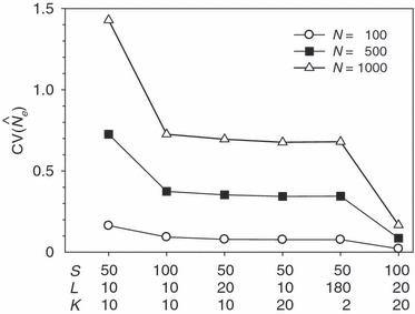
Effects of independently doubling sample size of individuals (S), number of loci (L), and number of alleles per locus (K) on the coefficient of variation (CV) of . Results are shown for three different population sizes of N ideal individuals. CV() was computed using eqn (3) in the text.

Equation (3) and Fig. 1 assume a fixed number of alleles per locus. In the simulated datasets, we specified the maximum number of allelic states per locus (A) but the actual number of segregating alleles (K) was a random variable. Figure 2 shows how the total number of (presumably independent) allelic combinations (n) in the simulated data varied with other input parameters. n increased sharply as lower frequency alleles were admitted into the computations and in general was about twice as high for P_crit = 0.05 as for 0.1 and about three times as high for P_crit = 0.02. Interestingly, for fixed values of L and A, the number of useful allelic combinations was not very sensitive to sample size or effective size (Fig. 2, top panel). For specified values of N, S, and L, n was much higher for A = 10 than A = 5 but did not increase much more with a larger number of potential allelic states (Fig. 2, middle panel). This result occurred because under the simulated conditions, most populations were not able to maintain much beyond 10 alleles per locus. With larger populations (N > 500–1000), increasing A beyond 10 allelic states did allow more alleles into the analysis, but the effect was not large (data not shown). Increasing the number of loci led to large increases in the number of allelic combinations (Fig. 2, bottom panel), a result directly attributable to the fact that the number of pairwise comparisons increases with the square of the number of loci.

Figure 2.

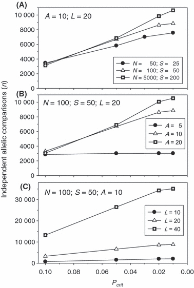
Changes in the number of independent allelic comparisons (n) available to compute mean as a function of the criterion for excluding rare alleles (P_crit). Results shown are means across replicates for simulated data using different combinations of population size (N), sample size (S), number of gene loci (L), and maximum number of alleles per locus (A). (A) Effects of variation in N and S with A and L fixed. (B) Effects of variation in A while N, S, and L are fixed. (C) Effects of variation in L while N, S, and A are fixed.

The practical consequences of varying input parameters on the distribution of estimates are seen in Fig. 3. With N = 100 and only moderate amounts of data (S = 50; L = 10), most estimates clustered around 100 and only 0.3% were higher than 500. A much tighter distribution of , with virtually all estimates falling between 50 and 150, was obtained with larger samples of individuals and loci (S = 100; L = 40). The bottom panel shows a much wider range of estimates for N = 1000 than N = 100. Under somewhat typical conditions (S = 50 and L = 20), when true N_e was 1000 over a third of the estimates were >2000. However, for N = 1000 only 1% of the were <300, and for N = 100 only 0.1% of the were >300. Thus, when using the LD method with an amount of data that it is currently possible to achieve for many natural populations, one is not likely to mistake a population with moderately small N_e for one with large N_e.

Figure 3.

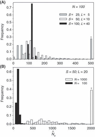
Empirical distribution of values for 1000 replicate simulated populations, as a function of population size (N), sample size (S), and number of gene loci (L). Each gene locus had a maximum of 10 alleles each, and the criterion for excluding rare alleles was P_crit = 0.02 (for S > 25) and P_crit = 0.03 (for S = 25). (A) Population size fixed at N = 100, while S and L vary. (B) Results for two different population sizes with S and L fixed at 50 and 20, respectively. Bins marked with an asterisk represent all estimates >500 (Panel A) or >2000 (Panel B).

A broader picture of practical applicability of the LD method can be obtained by examining data in Table 2, which shows the fraction of estimates that differ from N by a factor of 2x or 10x. One major result clearly illustrated here is that lower portions of the distribution of are much more constrained than upper portions. For example, assuming a standard sample of 20 ‘microsat’ loci and N = 500, even a sample of only 25 individuals is sufficient to ensure that will almost never be <10% of N. Conversely, with N = 500 and S = 25, about 25–30% of the estimates exceeded 10N = 5000, depending on the P_crit value used.

Precision is also strongly affected by interaction between sample size and effective size. When N is only 100, a sample of 25 individuals genotyped for 20 ‘microsat’ loci is sufficient to ensure that only a small fraction (1.6% for P_crit = 0.03; Table 2) of estimates will be less than half the true value. But with N = 500 and the same sample size and P_crit, about 25% of values will be <0.5N. This table thus illustrates that, for numbers of highly polymorphic loci typically available at present, small samples on the order of 25 individuals can provide meaningful information about effective size only for populations that are not too large (N_e < about 500). The practical value of small samples in the range S = 25 also depends heavily on the number of loci and alleles. For example, with only five ‘microsat’ loci typed, samples of S = 25 do not produce reliable estimates of N_e even when N is as small as 100 (most are either <<100 or >500; Fig. 3A).

Finally, results in Table 2 emphasize that even with large samples of individuals, the upper bound of is not well defined if N_e is large. With N = 100 a sample of 50 individuals is sufficient to ensure that no values are >10N, but with N = 1000 about 6% of estimates are >10N even when based on sample sizes of 100, and for N = 5000 even samples of 200 individuals produce a quarter or more of estimates with > 10N. Increasing the number of loci also helps precision (Table 2), but the problem of placing an upper bound on for large populations remains challenging.

Direct effects on precision when low-frequency alleles are used are seen in the second panels in Figs 4 and 5. For all values of N, CV() is highest for P_crit = 0.1, drops by about 40–50% for P_crit = 0.05, and declines further (but more modestly) for P_crit = 0.02 and 0.01. This effect is essentially independent of sample size.

Figure 4.

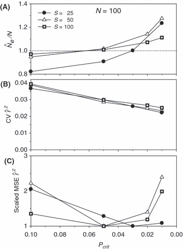
Indices of precision and bias for estimates of N_e for simulated data, plotted as a function of sample size (S) and the criterion for excluding rare alleles (P_crit). Results shown used 20 loci with a maximum of 10 alleles per locus, and population size was N = 100. (A) Bias in harmonic mean ; dotted line shows unbiased expectation = 1.0. (B) Coefficient of variation (CV) of , measured across 1000 replicate values computed as means across all 20 gene loci. (C) Mean-squared error (MSE) of , scaled within each sample size so that the lowest MSE = 1.0.

Figure 5.

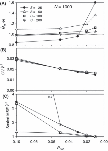
As in Fig. 4, but with N = 1000.

Bias

We found an interaction between bias (indexed by the ratio harmonic mean /N), S, and P_crit (Figs 4 and 5). In general, the LD method has little or no bias for P_crit ≥ 0.05, which is not surprising as the empirical bias correction (Waples 2006) was developed for data that excluded alleles at frequency <5%. As alleles with lower frequency are allowed into the analysis, estimates become biased slightly upwards, and this effect is more pronounced for smaller sample sizes (compare results for S = 50, 100, and 200 with N = 1000 in Fig. 5). The program Ldne implements a separate bias correction for S < 30; this reverses the trend of increasing upward bias with smaller samples and actually leads to a slight downward bias for P_crit ≥ 0.05 (Figs 4 and 5). However, this small-sample correction is not effective at the lowest P_crit considered (0.01), which (in the case of S = 25) fails to exclude any alleles, even those occurring in only a single copy. For this sample size, use of P_crit = 0.03, which screens out singletons but allows all other alleles into the analysis, led to essentially unbiased estimates of N_e for N ≤ 1000 (Figs 4 and 5). The effect of allowing singletons can also be seen for S = 50 in Figs 4 and 5, where upward bias rises sharply for P_crit = 0.01, a criterion that allows alleles that occur only once in a sample of 2S = 100 genes.

Results presented in Figs 2, 4, and 5 thus illustrate an inherent tradeoff between bias and precision: in general, a lower P_crit leads to estimates that are not only more precise but also more biased. MSE analyses (bottom panels in Figs 4 and 5) are useful to review in this context. P_crit = 0.1 is clearly too conservative, sacrificing too much precision for only modest benefits with respect to bias. Otherwise, which P_crit value leads to the lowest MSE depends to some extent on S and N: with N = 100, P_crit in the range 0.03–0.05 led to the lowest MSE, depending on sample size, whereas with N = 1000 the most extreme P_crit (0.01) produced the smallest MSE.

We found no appreciable effect of the number of loci on bias (data not shown). The maximum number of alleles per locus had little effect over the range A = 10–40, but upward bias in was largely eliminated with A = 5 (data not shown). Presumably, this occurred because A = 10 was sufficient to saturate our populations with rare alleles, whereas with only five alleles per locus most alleles remained at intermediate frequencies.

Collectively, results discussed above and for other parameter sets we considered suggest the following practical ‘rule of thumb’ for balancing the precision–bias tradeoff for the LD method: choose P_crit to be the larger of 0.02 or a value that screens out alleles that occur in only one copy. Operationally, this rule can be expressed as follows:

For S > 25: choose P_crit = 0.02.

For S ≤ 25: choose so that 1/(2S) < P_crit ≤ 1/S.

Adoption of this simple rule can be expected to lead to largely unbiased estimates of N_e that have relatively high precision under a wide range of conditions (Fig. 6). If this rule is followed, most realistic situations should produce estimates of N_e with bias <10% or so – a relatively small effect considering the various other sources of uncertainty associated with biological systems. Because rare alleles cause less upward bias in for large S, if sample size is about 100 or larger users might consider using P_crit = 0.01 to maximize precision with relatively little cost in terms of bias. This might be particularly effective in situations where population size is thought to be large, in which case adequate precision is difficult to achieve without a great deal of data. Note, for example, that with N as large as 5000, estimates based on samples <100 individuals become highly unreliable (Fig. 6).

Figure 6.

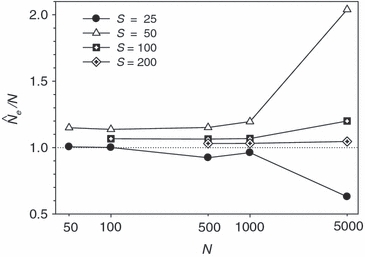
Bias in harmonic mean across replicate populations as a function of population size (N) and sample size (S). Dotted line shows unbiased expectation = 1.0. Results shown used 20 gene loci with a maximum of 10 alleles each, and the criterion for excluding rare alleles was P_crit = 0.02 (for S > 25) and P_crit = 0.03 (for S = 25).

Confidence intervals

Although confidence intervals to are easy to calculate for the LD method, they are complicated to evaluate. To illustrate, consider an idealized scenario in which the point estimate is unbiased (harmonic mean = N) and 95% of the 95% CIs contain the true value of N_e, which is fixed and equal to N every replicate. Practical realities lead to several types of departures from this ideal scenario.

Problem 1

Parametric CIs for the LD method are based on the observation that a function of is distributed approximately as chi-square with n degrees of freedom: CV²() ≍ 2/n (Hill 1981), with n defined as in eqn (1). However, this formulation assumes that the L(L−1)/2 pairwise comparisons among loci are all independent, which is not strictly true; correlations among overlapping pairs of loci (e.g., locus 1 with locus 2 and locus 1 with locus 3) violate this assumption (Hill 1981). As a consequence, variance of mean does not decrease as fast as the theoretical expectation when additional loci are used, and parametric confidence intervals based on the chi-square approximation (Equation 12 in Waples 2006) do not contain the true value the expected fraction of the time when many loci are used.

Problem 2

If is biased, CIs computed for replicate point estimates will tend to perform poorly because they are generated around the biased point estimates but are being compared to the unbiased (true) value of N_e. For example, if the estimator is biased toward high values (as occurs for the LD method with some combinations of N, S, and P_crit), the entire CI will be above the true value a disproportionate fraction of the time.

Problem 3

A somewhat related phenomenon, recently described by Waples and Faulkner (2009), is that when one explicitly models a Wright–Fisher ‘ideal’ population (e.g., in a computer model that tracks multilocus genotypes), the realized effective size in each replicate (N_e*) only rarely, and only by chance, equals the nominal ‘true’ value of N. This is because in the Wright–Fisher model, the realized variance among individuals in genes contributed to the next generation (V_k*) is a random variable; effective size equals N only when V_k* is exactly equal to the binomial expectation E(V_k) = 2(N−1)/N, so in most replicates N_e* is higher or lower than N because V_k* ≠ 2(N−1)/N. This effect is small if N is large but can be important even for N = 100, in which case realized N_e* typically varies between about 80 and 120 (± about 20%) across replicate generations in modeled ideal populations (Waples and Faulkner 2009). As a consequence of this effect, performance evaluations of CIs in modeled populations will tend to be overly pessimistic because they do not account for random variation in realized N_e*.

To recap, Problem 1 means that parametric CIs for the LD method will tend to be slightly too narrow, with the effect being more pronounced for large numbers of loci. Problems 2 and 3 remain even if the CIs have the appropriate width; these problems arise because the CIs are offset from the ‘true’ value of N_e. In Problem 2, the offset is a real bias and occurs consistently in one direction. In contrast, in Problem 3 the offset is not a bias but instead is due to random differences between realized N_e* and what is assumed to be the true, constant value N_e = N. Interestingly, and importantly, Problems 2 and 3 are both more acute with large amounts of data (high S, L, K). With only modest amounts of data, CIs will be wide and will (by chance) include N a large fraction of the time, even with bias in (Problem 2) or random variation in N_e* (Problem 3). However, as more and more data are brought into the analysis, the CIs will become narrowly focused on the biased point estimate (Problem 2) or the realized value of N_e* that applies to that particular replicate generation (Problem 3). In both cases, the resulting CIs will include N a smaller and smaller fraction of the time as information content increases. In contrast to Problem 1, which is specific to the LD method because it arises from a lack of independence of overlapping pairs of loci, Problems 2 and 3 are more generic and apply as well to confidence intervals for other N_e estimators.

What are practical implications of these factors? Waples and Do (2008) proposed a jackknife method to empirically estimate the variance of and modify parametric LD confidence intervals accordingly, which should address Problem 1 given an adequate number of loci to compute a jackknife estimate. Problem 3 complicates evaluation of performance of CIs with simulated data, which is one reason we do not provided detailed evaluations of CIs in this study. However, this problem arises from a type of pseudoreplication inherent to simulated data (Waples and Faulkner 2009) and therefore ceases to be a problem when considering data from natural populations, where each sample has associated with it only one realized N_e*, which is the parameter of interest. Problem 2 is therefore of most immediate concern for those interested in placing confidence limits on estimates of N_e in natural populations. The best approaches are to 1) pick a method that is unbiased, or 2) accept a small degree of bias in exchange for greater precision, recognizing that the resulting CIs might exclude the true N_e a higher-than-expected fraction of the time (even if the width of the CIs is appropriate).

The LD method versus the temporal method

Equations (3) and (4) allow a theoretical comparison of precision of the LD method and the moment-based temporal method. For both estimators, CV() is inversely related to the number of degrees of freedom; this is generally larger for the LD method because as the numbers of loci and alleles/locus increase, n increases as the square of L and K while the temporal n′ increases only linearly with L and K (compare eqns 1 and 5). Thus, we expect that precision should increase more rapidly for the LD method as more loci and alleles are used. Conversely, in the temporal method CV() declines with increasing time between samples (eqn 4), while this parameter does not affect LD estimates. Finally, although precision in both methods is lower for larger N, the coefficient for the N_e term is smaller for the temporal method (eqn 4) than for the LD method (eqn 3), indicating that precision for the temporal method should not decline as rapidly with increases in population size. These diverse and contrasting effects can be quantified by considering the ratio of the coefficients of variation for (CV_LD/CV_T). As the temporal method requires two samples of size S, to standardize the comparison we assumed a single sample of size 2S for the LD estimates (see Wang 2009, for a comparable adjustment for comparisons of two-sample and one-sample methods). With this adjustment and assuming K is constant, after combining eqns (3) and (4), expanding the expressions for n and n′ using eqns (1) and (5), and simplifying, yields:

(6)

With this formulation, values of the ratio >1 indicate that the temporal method has greater precision, while the LD method is more precise when the ratio <1. Obviously, this analysis is only meaningful for L ≥ 2 (a minimum of two loci are required for the LD method) and K ≥ 2 (monomorphic loci provide no information). It is easy to see that the first term in eqn (6) will be 1 if L,K = (3,2) or (2,3), and the ratio will be < 1 if either L or K >3. The numerator and denominator of the second term will be equal when t = 1.33 generations, and the numerator will be larger if the time between samples exceeds this value.

These effects are illustrated for some representative parameter combinations in Fig. 7. Relative performance of the temporal method increases (higher ratio) when (i) more generations elapse between samples (compare results for t = 2 and 10 for L = 5 loci, K = 5 alleles and L = 20, K = 10); (ii) smaller samples are used (compare results for S = 25 and 50 for L = 20, K = 10); and larger populations are involved (consistently higher ratios for N = 500 and 1000 than for N = 100). Conversely, increasing L and K has a dramatic effect on reducing CV_LD, leading to low values of the ratio. The only parameter combination for which overall precision was better for the temporal method involved modest amounts of data (five loci with five alleles each) and a relatively long time (10 generations) between samples. For the other (arguably more realistic) parameter combinations, precision of the LD method was higher, and often a great deal higher. For example, with 20 ‘microsat’ loci with 10 alleles each or 180 diallelic ‘SNP’ loci, CV_LD was a third lower than CV_T with N = 1000 and over two-thirds lower with N = 100 (Fig. 7).

Figure 7.

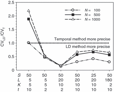
Theoretical precision of the LD and temporal methods for various combinations of parameters. Values on the Y-axis are ratios of coefficients of variation of for the LD method [CV_LD() from eqn 3] and the temporal method [CV_T() from eqn 4]. The dotted horizontal line identifies the point at which precision is the same for the two methods. Points above the line indicate greater precision for the temporal method, points below the line greater precision for the LD method. Variables considered are population size (N), sample size of individuals (S), number of loci (L), number of alleles per locus (K), and number of generations between samples (t, temporal method only). Results for the temporal method assume two samples each of size S and results for the LD method assume a single sample of size 2S.

These results should be regarded as only a general indication of relative precision of the two methods. Various estimators used in the temporal method have different variance properties, providing some opportunities to trade off precision and accuracy (Jorde and Ryman 2007). Furthermore, likelihood-based (Wang 2001) or approximate Bayesian computation (ABC; Tallmon et al. 2004) temporal methods should have lower variance than moment-based estimators, at least if their underlying assumptions are satisfied. Nevertheless, the general patterns observed here should be fairly robust. Notably, Wang (2009, Fig. 1) found qualitatively similar results in comparing his pseudo-likelihood temporal method to a new single-sample estimator (discussed below): the temporal method performed poorly for low t but eventually outperformed the single-sample estimator if the temporal samples were spaced a large enough number (t = 16–32) of generations apart, and doubling the number of loci led to larger increases in precision of the single-sample method.

Discussion

It seems clear that previous efforts to estimate effective size in natural populations have not extracted as much information as possible from genetic data. Any application of the temporal method that collects multilocus genotypic data provides an opportunity to obtain at least two estimates of N_e from individual generations using the LD method or one of the other single-sample estimators, but relatively few have taken advantage of this opportunity.

The simulation program used here (EasyPop) differs in some important ways from the one used to generate data to develop the empirical bias correction for the LD method (Waples 2006). In particular, the original program had no mutation and considered only diallelic loci at moderate allele frequency, whereas EasyPop has an explicit mutation model and generates data with a wide range of allele frequencies and numbers of alleles per locus. The new simulated data thus represent an independent assessment of the bias-corrected LD estimator – and a more realistic assessment of performance with highly polymorphic markers currently in widespread use. In summarizing important results of our evaluations, we return to the specific questions posed in the Introduction before closing by discussing a few related issues.

Factors affecting precision and bias

The LD method benefits from the fact that the amount of information increases with the square of the numbers of loci and alleles, so efforts to capitalize on ready availability of highly variable markers can pay large dividends. Within the range of values of practical interest to most investigators, the same proportional increases in numbers of loci, alleles per locus, or individuals sampled should have roughly comparable effects on precision, and this result (along with the quantitative expression for CV_LD in eqn 3) can be used to guide experimental design decisions. Although each SNP locus provides much less precision than a typical microsatellite, this can be overcome by brute force if enough new independent loci can be developed. Figure 1 indicates that about 180 SNP loci can be expected to provide precision comparable to that attained by about 10–20 typical microsatellite loci; this might seem like a lot, but techniques to develop thousands of SNP loci are rapidly advancing and declining in cost (Morin et al. 2004; Xu et al. 2009). As discussed below (Key assumptions), however, an application using a very large numbers of SNP loci should be accompanied by a careful analysis of assumptions of independence and neutrality.

Rare alleles tend to upwardly bias LD estimates of N_e, just as they do for the temporal method (Turner et al. 2001), but in many cases the effect is not too severe. This means that large numbers of alleles typically can be allowed into the analysis to boost precision without substantially increasing bias. For most applications, a good rule of thumb is to screen out any alleles at frequency <0.02, as well as any alleles that occur in only a single copy in the sample (see Nielsen and Signorovitch 2003, for discussion of effects on of using singletons from SNP data). Using this criterion, something close to maximum precision can be achieved while (in most cases) keeping bias to less than about 10% (Fig. 6). With large samples (S∼ 100 or larger), alleles with frequency as low as 0.01 can probably be used.

Practical applications

All genetic methods for estimating contemporary depend on a signal that is a function of 1/N_e, so these methods are most powerful with small populations (for which the signal is strong) and have difficulty distinguishing large populations from infinite ones (because the signal is so small). This effect is amply demonstrated for the LD method in Figs 1 and 3 and Table 2. With amounts of data commonly available today (samples of about 50 individuals; 10–20 microsatellite-like loci), quite good precision can be obtained for populations with relatively small effective sizes (about 100–200 or less). For very small populations (N_e less than about 50), small samples of only 25–30 individuals can still provide some useful information. These results are encouraging, as conservation concerns typically focus on populations that are (or might be) small, and modern molecular methods have facilitated an increasing interest in studying evolutionary processes in local populations in nature.

In contrast, estimating effective size with any precision in populations that are large (N_e∼ 1000 or larger) is very challenging. In general, a small sample of individuals (or a moderate or large sample based on only a few gene loci) will not provide much useful information about N_e in large populations, and even with relatively large samples of individuals and loci it might not be possible to say much about the upper bound to . In theory, with arbitrarily large numbers of loci and alleles (as might routinely be achievable in the future), it should be possible to produce estimates that place tight bounds even on the upper limit to in large populations (cf. Fig. 1). However, because the drift signal is so small for large populations, researchers who want to estimate N_e in populations that are or might be large should pay careful attention to various sources of noise in the analysis (slight departures from random sampling; data errors; violation of underlying model assumptions) that can have a disproportionate effect on results. In this respect, estimating contemporary N_e in large populations using genetic markers is as challenging as, and suffers many of the same intrinsic limitations as, genetic estimates of dispersal in high gene flow species (Waples 1998; Fraser et al. 2007). Fortunately, because the LD signals for large and small populations are quite different (Fig. 3), estimates based on even moderate amounts of data should be able to provide a useful lower bound for N_e, and this can be important, particularly in conservation applications where a major concern is avoidance and/or early detection of population bottlenecks.

Based on extensive computer simulations, Russell and Fewster (2009) reached a rather pessimistic conclusion about practical usefulness of the LD method. However, two factors make their results difficult to interpret in the present context. First, they presented quantitative results only for the original LD method (Hill 1981) which, when the ratio S/N_e is small, has been shown to produce an estimate that is more closely related to the sample size than to the true effective size (England et al. 2006; Waples 2006). Second, Russell and Fewster (2009) assessed bias by comparing arithmetic mean to the true N_e. Because of the inverse relationship between and (eqn 2a), this has the unfortunate consequence that if is a completely unbiased estimator of r², arithmetic mean will be upwardly biased. Results in Table 2 and Figure 3 show how upwardly skewed the distribution of can be, in which case the arithmetic mean is not a useful indicator of central tendency. Here, we have followed the approach used by Nei and Tajima (1981), Pollak (1983), Waples (1989), Jorde and Ryman (2007), Nomura (2008), and Wang (2009), all of whom evaluated bias in terms of harmonic mean (or, equivalently, used the overall mean or temporal across replicates to compute an overall ). Importantly, this approach can readily accommodate negative or infinite values in individual replicates (see next section).

Negative estimates and nonsignificant LD

As shown in eqn (2a), before estimating N_e in the LD method, the expected contribution of sampling error is subtracted from the empirical . If N_e is large, or if only limited data are available, by chance mean can be smaller than the sample size correction, in which case the estimate of N_e will be negative. A related phenomenon can occur with the standard temporal method (Nei and Tajima 1981; Waples 1989) and with unbiased estimators of genetic differentiation (Nei 1978; Weir and Cockerham 1984). Negative estimates occur when the genetic results can be explained entirely by sampling error without invoking any genetic drift, so the biological interpretation is = ∞ (Laurie-Ahlberg and Weir 1979; Nei and Tajima 1981). In this situation, the user can conclude that the data provide no evidence that the population is not ‘very large’. However, even if the point estimate is negative, if adequate data are available the lower bound of the CI generally will be finite and can provide useful information about plausible limits N_e.

Many software packages provide tests of statistical significance of LD for each pair of loci or across all loci. Although these tests vary in the way they assess significance and combine information across multiple alleles and loci, in general they are testing the hypothesis that the observed LD can be explained entirely by sampling error. A nonsignificant test for LD, therefore, indicates that the null hypothesis (H₀: ≤ 1/S) cannot be rejected, which implies that the upper bound of would include infinity. That is, a nonsignificant test provides no evidence for drift, which is not the same as saying no drift occurs (in fact, all finite populations have some contribution to from drift, and, assuming the test is valid, that drift component should become statistically significant if enough data are collected). So, for reasons discussed in the previous paragraph, even a dataset with a nonsignificant LD result can potentially provide useful information about effective population size.

Key assumptions

Like other N_e estimators, the LD method assumes that of the four evolutionary forces (mutation, migration, selection and genetic drift), only drift is responsible for the signal in the data. Although mutation rate strongly affects estimates of long-term N_e, it probably is of little consequence for the LD method, apart from its role in producing genetic variation. Selection can cause nonrandom associations of genes at different gene loci, just as it can influence rates of allele frequency change, but it might be reasonable to assume that it has relatively little influence on LD measured in microsatellite loci. The neutrality assumption should be evaluated more rigorously, however, if large numbers of SNP loci are used. Vitalis and Couvet (2001) proposed a method to jointly estimate N_e and migration rate. Immigration of genetically differentiated individuals from other populations leads to mixture disequilibrium (Nei and Li 1973) that could downwardly bias LD estimates of local N_e; conversely, high migration rates among weakly differentiated populations could cause local samples to provide an estimate closer to the metapopulation N_e than the local N_e (because the sample is drawn from a larger pool of potential parents). Unpublished data (P. England, personal communication) indicate that under equilibrium migration models, the former effect is small and the latter effect is substantial only for migration rates that are high in genetic terms (∼10% or higher) – suggesting that under many natural conditions the LD method can provide a robust estimate of local (subpopulation) N_e. However, upward biases in might be more important in small subpopulations that are part of a metapopulation, as in that case even a few migrants per generation could represent a relatively high migration rate.

The LD method as implemented here assumes that loci are independent (probability of recombination = 0.5). This is probably a reasonable assumption in most current situations, given the numbers of markers typically used in studies of natural populations. However, some taxa (e.g., Drosophila) have only a few chromosomes and/or regions of the genome in which recombination is suppressed, and in the future LD estimates might be generated using thousands of SNP or other markers. In such cases, therefore, issues related to recombination rate would have to be re-evaluated. Linked markers actually provide more power, providing the recombination rate is known (Hill 1981). The LD method provides information primarily about N_e in the parental generation, but residual disequilibrium from a recent bottleneck can affect the estimate for a few generations (Waples 2005, 2006). If loci are closely linked, estimates from the LD method will be more strongly influenced by N_e in the distant past (see Tenesa et al. 2007, for an application to human SNP data).

The theoretical relationship between and N_e assumes either random mating without selfing or random mate choice with lifetime monogamy (Weir and Hill 1980; Waples 2006). The populations do not have to be ideal; the method still performs well with highly skewed sex ratios and overdispersed variance in reproductive success (Waples 2006). However, strongly assortative mating or widespread selfing would be expected to lead to biases that have not been quantitatively evaluated. Genotyping errors can also affect estimates of LD (Akey et al. 2001). Russell and Fewster (2009) found an upward bias in for the standard LD method (Hill 1981) when 1% allelic dropout was modeled, and this topic bears further study.

Finally, the underlying model for the LD method assumes discrete generations, and this is the only situation where the resulting estimate can be interpreted as effective size for a generation (N_e). Most natural populations do not have discrete generations; when samples are taken from age-structured species, the resulting estimate from the LD method can be interpreted as an estimate of the effective number of breeders (N_b) that produced the cohort(s) from which the sample was taken. The relationship between and N_e in age-structured species has been evaluated for the temporal method (Waples and Yokota 2007), but comparable evaluations have not been made for any single-sample estimator. A reasonable conjecture is that if the number of cohorts represented in a sample is roughly equal to the generation length, the estimate from the LD method should roughly correspond to N_e for a generation, but this remains to be tested.

Comparison with other methods

As illustrated in Fig. 7, with samples of individuals, loci, and alleles routinely available today, the LD method should generally provide better precision than the temporal method, unless samples for the latter are spaced a large number of generations apart.

Several other one-sample estimators of N_e have been proposed, although direct comparisons of performance have generally not been made with the LD method. The heterozygote excess method is generally much less precise than other single-sample estimators (Nomura 2008; Wang 2009) and is best suited for analyzing small populations of species with Type III survivorship for which large samples of offspring are possible (Hedgecock et al. 2007; Pudovkin et al. 2009). A single-sample ABC estimator (OneSamp; Tallmon et al. 2008) appears to have considerable potential but has not been rigorously evaluated under a wide range of conditions and assumes a specific type of mutation model that makes it useful only for microsatellite data. Two new methods, based on the analysis of molecular coancestry (Nomura 2008) and identification of full and half sibs (Wang 2009), each included some comparisons with some other N_e estimators. However, Nomura only considered populations with tiny N_e (<15) and only compared his new method to the heterozygote excess method, which was also the only single-sample estimator that Wang (2009) compared his new method to with simulated data.

Nevertheless, Wang did provide results for some analyses that are comparable enough to those conducted here that a quantitative comparison of the LD method and the sibship method is possible for a few parameter combinations. In Table 5 of his paper, Wang (2009) reported the root mean-squared error () for the quantity for simulations using random mating populations of constant size with equal sex ratio and 10–40 gene loci with eight alleles of initial equal frequency. That analysis involved a comparison with temporal samples taken in generations 3 and 5, so to get a single sibship-based estimate for each replicate Wang computed an estimate for both generations and took the average. For the parameters N = 200, S = 50, L = 20, for the sibship method was 0.0005. To allow a comparison, we simulated populations as described in Methods with N = 200, L = 20, A = 8, and drew samples after 10 generations – long enough for levels of LD to stabilize. The version of EasyPop we used does not allow sampling in two different generations, so we used the approach described above of taking a single sample of twice the size (i.e., we sampled 100 individuals once rather than 50 individuals twice). All else being equal, the two sampling schemes should provide roughly comparable precision. For our simulated datasets, we found that of was 0.0004, slightly lower than the value reported by Wang for his one-sample method and considerably less than the value he found (0.0015) for temporal samples separated by two generations. For the same set of simulated populations and sample size S = 100 (two samples of 100 for the sibship method, one sample of 200 for the LD method), we found of 0.00025 compared to 0.0003 reported by Wang. It would be a mistake to place too much emphasis on these results, given that tabular values in Wang (2009) are rounded off and that the direct comparisons that are possible cover only a small fraction of potential parameter space. Nevertheless, these data suggest that LD and sibship one-sample methods might have roughly comparable levels of performance as measured by some common indicators. A comprehensive comparison of performance of the LD, coancestry, and sibship methods would be useful.

Combining estimates across methods

Researchers who have reported estimates of N_e from more than one method too often have not taken advantage of another opportunity to increase precision – combining the estimates into a single estimator. Because all the estimators respond to a signal that is inversely related to N_e, an appropriate way to combine estimates across methods would be to take a weighted harmonic mean (Waples 1991). Ideally, the weights would be reciprocals of variances, which can be obtained for the moment-based LD and temporal methods from eqns (3) and (4), respectively. Combining data for these two methods could be particularly useful for large populations, as the temporal method is somewhat less sensitive to large N. Appendix A provides a worked example of how effective size estimates can be combined, both within and across methods. Additional work would be needed to determine the most appropriate way to weight estimates from different single-sample estimators. However, Nomura (2008) showed that considerable improvements in performance can be obtained even by taking an unweighted harmonic mean of from the heterozygote excess and molecular coancestry methods.

Some cautions are important to keep in mind here. First, which time period(s) each estimate applies to needs careful consideration. Each of the single-sample estimators is most closely related to inbreeding N_e and provides an estimate of the effective number of breeders (N_b) that produced the sample (Waples 2005). Combining estimates from single-sample methods should therefore be straightforward, provided an appropriate weighting scheme can be developed. However, in general the single-sample and temporal methods do not provide estimates of N_e in exactly the same generations (Waples 2005). Each single-sample estimate relates to N_e in a single generation (or N_b for a particular time period), while a temporal estimate depends on the harmonic mean N_e in the entire interval spanned by the samples. If N_e does not vary too much over time and the primary interest is an overall estimate of effective size for the population, then it might be reasonable to simply combine the temporal and single-sample estimates with appropriate weights as discussed above. However, if the primary interest is N_e in specific generations, which might vary considerably, then careful consideration is needed to determine whether combining estimates is desirable.

Second, the benefits of combining estimates depend on the degree to which they provide independent information about effective size. Based on unpublished data cited by Waples (1991), the LD and temporal methods are essentially independent, but correlations among the other estimators have not been determined. Conducting these evaluations should be an important research priority.

Third, the different N_e estimators generally depend on similar, but not identical, suites of assumptions (as discussed above). It will generally be the case that not all of these assumptions are completely satisfied in any particular dataset, and the different estimators might behave in different ways in response to violation of these assumptions. Researchers should think carefully before combining estimates in cases for which good reasons exist to believe some key assumptions are strongly violated.

Appendices

Appendix A: Combining different estimates of effective size

Before attempting to combine different estimates of effective size, one should consider two questions posed at the end of the Discussion: Do the estimates apply to the same time period, or (if not) are they estimating the same ‘average’ quantity? And, Is it likely that violation of underlying assumptions has differentially affected some of the estimates? Assuming that it is reasonable to compute a combined estimate, two related issues must be considered: how to combine estimates of the same type (single-sample or temporal), and how to combine estimates across methods. These issues are discussed below in the worked example, but before doing so we describe two general principles that should be followed.

First, in combining estimates the harmonic mean should be used, for two reasons: (i) The distribution of can be highly skewed, in which case the arithmetic mean is not a useful indication of central tendency. In addition, it is problematical to take an arithmetic mean of a series that can include values that are negative or infinite. (ii) Taking the harmonic mean of a series of values based on is mathematically equivalent to taking the arithmetic mean of the and using that to estimate . It is easy to show analytically that this is true in general, and the general principle can be illustrated with a simple example. Assume one has three LD estimates of N_e, all based on samples of S = 50 individuals and comparable numbers of loci and alleles. Assume also that the mean values for the three samples are as follows: 0.04, 0.015, 0.025. In that case, a reasonable approach would be to calculate an overall mean as (0.04 + 0.015 + 0.025)/3 = 0.02667; this is exactly analogous to the way a mean is obtained for a single sample by averaging across many pairs of alleles. Use of = 0.02667 along with S = 50 in Equation 2a leads to = 1/[3*(0.02667−0.02)] = 50. We can compare this with the method that computes a separate for each sample and takes their harmonic mean. In that case, and again using Equation 2a for simplicity rather than the more complicated bias corrected expectations (Waples 2006), the three estimates become 16.667, −66.667, and 66.667. Although some popular software programs won't compute the harmonic mean of a series that includes a negative number, this is easily accomplished using the simple formula

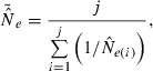(A1)

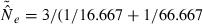
where j is the number of estimates. Note that this produces a result identical to that obtained by first averaging the individual values: = 50. In this situation, the arithmetic mean does not produce a sensible result, and simply ignoring infinite or negative estimates leads to downward bias in the composite estimate of N_e.

The other general principle to follow in combining estimates is that, whenever possible, the individual estimates should be weighted, with higher weights used for more precise estimates. Ideally, this would be done by making the weights proportional to reciprocals of variances. If a series of estimates are to be combined, and if V_i is the variance of for the i^th estimate, then the appropriate weights are

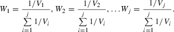(A2)

The weighted harmonic mean then is computed as

(A3)

A worked example

To illustrate these principles, we consider a subset of the data presented by Saarinen et al. (2009) for the Miami blue butterfly (Cyclargus thomasi bethunebakeri). We focus on the natural population BHSP, which was sampled in both 2005 and 2006 (S = 24 and 39 individuals, respectively), during which time an estimated t = 8 generations elapsed. These two samples were used to estimate N_e using three variations of the temporal method: the standard moment-based estimator (Waples 1989); another moment-based estimator using a modified formula for the temporal variance F (Jorde and Ryman 2007); and a pseudo maximum-likelihood estimator (Wang 2001). In addition, each of the samples was used to estimate N_e using two different single-sample estimators: the moment-based estimator LDNe and the ABC estimator OneSamp. Table A1 shows the estimates reported by Saarinen et al. (2009). For simplicity, we show only the LDNe estimates that used P_Crit= 0.02 and the OneSamp results with priors for N_e of 6-500 (the authors considered other variations, but results did not differ dramatically).

Table A1.

Combining estimates of N_e within methods (single-sample or temporal)

					Temporal
		Single-sample			Moment
Time	S	LD	ABC		W	JR	ML
2005	24	23.8	34.7	28.2	20.9	28	322
2006	39	35.9	29.3	32.3
HMean	29.7			30.7*	23.9†		44.6‡

^*Harmonic mean single-sample estimate for 2005 and 2006 combined () weighted by sample size and number of allelic comparisons (n).

^†Harmonic mean of the W and JR estimates ().

^‡Harmonic mean of the ML estimate and [the harmonic mean of the W and JR estimates] ().

HMean, harmonic mean; S, sample size; LD, linkage disequilibrium (Waples and Do 2008); ABC, Approximate Bayesian Computation (Tallmon et al. 2008); W, Waples (1989); JR, Jorde and Ryman (2007); ML, pseudo maximum likelihood (Wang 2001). This example uses data for the Miami blue butterfly from Saarinen et al. (2009).

Combining estimates within a method

The first step is to combine estimates within a method, and we begin with the two single-sample estimates. Although Hill (1981) provided an approximation for based on the LD method, a comparable expression is not available for the ABC method. In that situation, and absent any other quantitative way of assessing relative precision of the estimates, one can take an unweighted harmonic mean of the two values (equivalent to using j = 2 and setting both weights to 0.5 in Equation A3). Results are shown in Table A1: = 28.2 is the unweighted harmonic mean of the two single-sample estimates (23.8, 34.7) for 2005 and = 32.3 is the comparable result for 2006.

If one wants to combine single-sample and temporal estimates (see next section), one first has to compute an overall that applies to both of the single samples. We compute a weighted harmonic mean based on the theoretical variance of in the two time periods, using a simple modification of Equation 3 to compute the weights:

(A4)

This variance applies specifically to the LD method, but for lack of quantitative information regarding precision of the ABC method we use it for the combined LDNe + OneSamp estimates as well. Two factors differ between the 2005 and 2006 samples relevant to this variance: sample size (larger in 2006; Table A1) and number of allelic combinations (n = 715 in 2005 and 640 in 2006; Saarinen et al. 2009). Inserting these values into Equation A4 and setting N_e = 30.1 (unweighted harmonic mean over the 2 years) produces = 58 for 2005 and 31 for 2006. Using Equation A2 the weights thus become W₂₀₀₅ = 0.35 and W₂₀₀₆ = 0.65 and the weighted harmonic mean single-sample estimate (from Equation A3) thus becomes

= 1/(0.35/28.2 + 0.65/32.3) = 30.7.

The temporal method produces a single estimate that applies to the time period spanned by the samples, and the three different estimates obtained by Saarinen et al. (2009) are shown in Table A1. It is apparent that the two moment-based estimates are similar to the single-sample estimates, while the ML estimate is an order of magnitude higher. Jorde and Ryman (2007) found their revised estimator less biased but also less precise than the standard method, so it might be possible to develop a quantitative weighting for combining those two moment-based estimates. However, an expression for is not available, so for simplicity we use an unweighted approach. Biological considerations suggest three different strategies for doing this.

Strategy 1: Treat each estimate independently with equal weight and take an overall harmonic mean. With the three weights equal at W_i = 0.333, use of Equation A3 gives the harmonic mean temporal estimate as

Strategy 2: The two moment-based estimators might be considered to be largely redundant, so they could be combined before combing with the ML estimate. In this two-step process, the harmonic mean of the two moment-based estimates is first computed (23.9; Table A1), and then an unweighted harmonic mean is taken of this value and the ML estimate (322), producing the result

Strategy 3: The ML estimate seems to be an outlier and might be affected by small sample sizes, as suggested by Jorde and Ryman (2007). If the ML estimate is excluded, the combined temporal estimate is simply

In the present case, there does not appear to be a compelling reason for choosing among these options, so we consider Strategies 2 and 3 in the analyses below.

Combining estimates across methods

If one is primarily interested in estimates of N_e in specific generations, which might vary considerably over time, then it could be risky or misleading to try to combine temporal and single-sample estimates. On the other hand, if one is interested in an overall estimate of effective size that is expected to fluctuate only moderately around a mean value, then combining estimates from the two methods could be useful. Two factors argue for caution in doing this in the present example: (i) the temporal samples span eight generations, while the single-sample estimators provide information only about N_e at the beginning and end of this period; (ii) census size varies widely over time in this species (Saarinen et al. 2009), so it seems unlikely that the temporal and single-sample methods are estimating the same quasi-constant quantity. Nevertheless, for the sake of illustration we consider how information from these two methods could be combined.

The analogue to Equation A4 for the temporal method, slightly modified from Equation 4, is

(A5)

To calculate the variances and the respective weights, we need values for S, t, n, n’, and N_e. For S we used the harmonic mean for the 2 years (29.7), and for t we used eight generations. Saarinen et al. (2009) did not provide the total number of independent alleles (n’) used in the temporal estimates, but they were based on 11 of the 12 loci considered (the other being monomorphic at site BHSP in 1 year). Accordingly, we assumed each locus had five total alleles, which produced n = 880 (from Equation 1; close to the number reported for 2005) and n’ = 44 (from Equation 5). Because relative precision of the LD and temporal methods also depend on N_e (which is unknown) we considered three values that span the range of most of the empirical estimates: 25, 50, 100.

Results of these analyses are shown in Table A2, where we see that (given the S, n, and n’ values in this example) relative precision for the one- and two-sample methods is expected to be nearly the same for N_e = 50, with the LD method having a lower variance for N_e < 50 and the temporal method having a lower variance for larger N_e. As a result, the single-sample estimate gets higher weight than the temporal estimate for N_e = 25 (W_SS = 0.7; W_T = 0.3), while the temporal estimate receives greater weight for N_e = 100. Under Strategy 2, the combined temporal estimate is = 44.6 while the combined single-sample estimate is = 30.7 (Table A1). If, for example, we assume that true N_e = 25, the overall combined estimate across methods is calculated as

Table A2.

Combining estimates of N_e across single-sample (SS) and temporal (T) methods

	Effective population size
	25	50	100
Sample size (S)	29.7	29.7	29.7
Number of loci (L)	11	11	11
Alleles/locus (K)	5	5	5
n	880	880	880
n′	44	44	44
Generations (t)	8	8	8
Var()	18	208	2801
Var()	42	229	1542
WSS	0.70	0.52	0.36
WT	0.30	0.48	0.64
with ML	33.8	36.0	38.4
without ML	28.3	27.0	25.9

Results are shown for three different effective population sizes. is the weighted harmonic mean of the overall estimates for the two methods from Table A1 [= 30.7 for single-sample method and 44.6 or 23.9 for the temporal method with or without the Wang (2001) ML estimate, respectively].

n = number of degrees of freedom for the LD method (Equation 1); n’ = number of degrees of freedom for the temporal method (Equation 5); W = relative weights for single-sample and temporal estimates.

For N_e = 50 and 100, the corresponding estimates are = 36.0 and 38.4, respectively (Table A2). Note that for larger assumed N_e, the overall estimate moves closer to the value from the temporal method ( = 44.6), reflecting the higher relative weights for the temporal estimate. Under Strategy 3, the combined temporal estimate is lower ( = 23.9, Table A1), as is the combined estimate across methods () = 28.3, 27.0, 25.9 under the assumption that true N_e is 25, 50, 100 respectively). Again, the overall combined estimate moves closer to the temporal estimate for larger population size.

Comments

The above example illustrates some of the basic principles that should be considered if one is interested in combining different estimates of effective size. Nomura (2008) showed that taking even a simple unweighted harmonic mean of estimates from two one-sample methods can be effective, but performance should improve through use of an appropriate weighting scheme. As should be clear from the above example, deciding on appropriate weights can be tricky. Here are some additional factors that should be considered; the last two in particular merit additional research.

Sample size

Both in calculating and appropriate weights, one should use realized sample size—that is, the number of individuals for which genetic data were actually collected. If this varies across loci or pairs of loci, the harmonic mean realized sample size should be used. Saarinen et al. (2009) only reported the number of individuals collected so that is what we show in Table A1 and used in the example, but the harmonic mean realized sample size is provided as output by some software programs.

Confidence intervals

Although parametric confidence intervals are easy to calculate for both temporal and LD methods, obtaining confidence intervals for combined estimates is not straightforward. Doing so would require information not only about relative variances associated with the estimates but also the degree to which the different estimates provide independent information about effective size.

Precision and bias

The new temporal estimator proposed by Jorde and Ryman (2007) is less biased but also less precise than other temporal methods, and this paper also describes a tradeoff between bias and precision of the LD method regarding the criterion for screening out rare alleles. These observations suggest that it might be profitable to explore performance of an alternative weighting scheme based on MSE or RMSE rather than just the variance of .

Literature cited

- Akey JM, Zhang K, Xiong M, Doris P, Jin L. The effect that genotyping errors have on the robustness of common linkage disequlibrium measures. American Journal of Human Genetics. 2001;68:1447–1456. doi: 10.1086/320607. [DOI] [PMC free article] [PubMed] [Google Scholar]
- Balloux F. EasyPop (version 1.7): a computer program for population genetics simulations. Journal of Heredity. 2001;92:301–302. doi: 10.1093/jhered/92.3.301. [DOI] [PubMed] [Google Scholar]
- Balloux F. Heterozygote excess in small populations and the heterozygote-excess effective population size. Evolution. 2004;58:1891–1900. doi: 10.1111/j.0014-3820.2004.tb00477.x. [DOI] [PubMed] [Google Scholar]
- Charlesworth B. Effective population size and patterns of molecular evolution and variation. Nature Reviews Genetics. 2009;10:195–205. doi: 10.1038/nrg2526. [DOI] [PubMed] [Google Scholar]
- England PR, Cornuet J-M, Berthier P, Tallmon DA, Luikart G. Estimating effective population size from linkage disequilibrium: severe bias using small samples. Conservation Genetics. 2006;7:303–308. [Google Scholar]
- Frankham R. Genetics and extinction. Biological Conservation. 2005;126:131–140. [Google Scholar]
- Fraser D, Hansen MM, Østergaard S, Tessier N, Legault M, Bernatchez L. Comparative estimation of effective population sizes and temporal gene flow in two contrasting population systems. Molecular Ecology. 2007;16:3866–3889. doi: 10.1111/j.1365-294X.2007.03453.x. [DOI] [PubMed] [Google Scholar]
- Hedgecock D, Launey S, Pudovkin AI, Naciri Y, Lapègue S, Bonhomme F. Small effective number of parents (Nb) inferred for a naturally spawned cohort of juvenile European flat oysters Ostrea edulis. Marine Biology. 2007;150:1173–1182. [Google Scholar]
- Hedrick PH. Gametic disequilibrium: proceed with caution. Genetics. 1987;117:331–341. doi: 10.1093/genetics/117.2.331. [DOI] [PMC free article] [PubMed] [Google Scholar]
- Hill WG. Estimation of linkage disequilibrium in randomly mating populations. Heredity. 1974;33:229–239. doi: 10.1038/hdy.1974.89. [DOI] [PubMed] [Google Scholar]
- Hill WG. Estimation of effective population size from data on linkage disequilibrium. Genetical Research. 1981;38:209–216. [Google Scholar]
- Hudson RR. The sampling distribution of linkage disequilibrium under an infinite allele model without selection. Genetics. 1985;109:611–631. doi: 10.1093/genetics/109.3.611. [DOI] [PMC free article] [PubMed] [Google Scholar]
- Jorde PE, Ryman N. Unbiased estimator for genetic drift and effective population size. Genetics. 2007;177:927–935. doi: 10.1534/genetics.107.075481. [DOI] [PMC free article] [PubMed] [Google Scholar]
- Krimbas CB, Tsakas S. The genetics of Dacus oleae V. Changes of esterase polymorphism in a natural population following insecticide control—selection or drift? Evolution. 1971;25:454–460. doi: 10.1111/j.1558-5646.1971.tb01904.x. [DOI] [PubMed] [Google Scholar]
- Laurie-Ahlberg C, Weir BS. Allozyme variation and linkage disequilibrium in some laboratory populations of Drosophila melanogaster. Genetical Research. 1979;32:215–229. doi: 10.1093/genetics/92.4.1295. [DOI] [PMC free article] [PubMed] [Google Scholar]
- Leberg P. Genetic approaches for estimating the effective size of populations. Journal of Wildlife Management. 2005;69:1385–1399. [Google Scholar]
- Maruyama T. Stochastic integrals and their application to population genetics. In: Kimura M, editor. Molecular Evolution, Protein Polymorphism, and the Neutral Theory. Berlin: Springer-Verlag; 1982. pp. 151–166. [Google Scholar]
- Morin PA, Luikart G, Wayne RK. SNPs in ecology, evolution and conservation. Trends in Ecology and Evolution. 2004;19:208–216. [Google Scholar]
- Nei M. Estimation of average heterozygosity and genetic distance from a small number of individuals. Genetics. 1978;89:583–590. doi: 10.1093/genetics/89.3.583. [DOI] [PMC free article] [PubMed] [Google Scholar]
- Nei M, Li W-H. Linkage disequilibrium in subdivided populations. Genetics. 1973;75:213–219. doi: 10.1093/genetics/75.1.213. [DOI] [PMC free article] [PubMed] [Google Scholar]
- Nei M, Tajima F. Genetic drift and estimation of effective population size. Genetics. 1981;98:625–640. doi: 10.1093/genetics/98.3.625. [DOI] [PMC free article] [PubMed] [Google Scholar]
- Nielsen R, Signorovitch J. Correcting for ascertainment biases when analyzing SNP data: applications to the estimation of linkage disequilibrium. Theoretical Population Biology. 2003;63:245–255. doi: 10.1016/s0040-5809(03)00005-4. [DOI] [PubMed] [Google Scholar]
- Nomura T. Estimation of effective number of breeders from molecular coancestry of single cohort sample. Evolutionary Applications. 2008;1:462–474. doi: 10.1111/j.1752-4571.2008.00015.x. [DOI] [PMC free article] [PubMed] [Google Scholar]
- Nunney L, Elam DR. Estimating the effective population size of conserved populations. Conservation Biology. 1994;8:175–184. [Google Scholar]
- Palstra FP, Ruzzante DE. Genetic estimates of contemporary effective population size: what can they tell us about the importance of genetic stochasticity for wild population performance? Molecular Ecology. 2008;17:3428–3447. doi: 10.1111/j.1365-294x.2008.03842.x. [DOI] [PubMed] [Google Scholar]
- Pollak E. A new method for estimating the effective population size from allele frequency changes. Genetics. 1983;104:531–548. doi: 10.1093/genetics/104.3.531. [DOI] [PMC free article] [PubMed] [Google Scholar]
- Pudovkin AI, Zaykin DV, Hedgecock D. On the potential for estimating the effective number of breeders from heterozygote-excess in progeny. Genetics. 1996;144:383–387. doi: 10.1093/genetics/144.1.383. [DOI] [PMC free article] [PubMed] [Google Scholar]
- Pudovkin AI, Zhdanova OL, Hedgecock D. Sampling properties of the heterozygote-excess estimator of the effective number of breeders. Conservation Genetics. 2009 doi: 10.1007/s10592-009-9865-5 (published online 7 March 2009) [Google Scholar]
- Russell JC, Fewster RM. Evaluation of the linkage disequilibrium method for estimating effective population size. In: Thomson DL, Cooch EG, Conroy MJ, editors. Modeling Demographic Processes in Marked Populations Environmental and Ecological Statistics. Vol. 3. Berlin: Springer; 2009. pp. 291–320. [Google Scholar]
- Schwartz MK, Tallmon DA, Luikart GH. DNA-based Ne estimation: many markers, much potential, uncertain utility. Animal Conservation. 1999;2:320–322. [Google Scholar]
- Schwartz MK, Luikart G, Waples RS. Genetic monitoring: a promising tool for conservation and management. Trends in Ecology and Evolution. 2007;22:25–33. doi: 10.1016/j.tree.2006.08.009. [DOI] [PubMed] [Google Scholar]
- Tallmon DA, Luikart G, Beaumont MA. Comparative evaluation of a new effective population size estimator based on approximate Bayesian computation. Genetics. 2004;167:977–988. doi: 10.1534/genetics.103.026146. [DOI] [PMC free article] [PubMed] [Google Scholar]
- Tallmon DA, Koyuk A, Luikart G, Beaumont MA. OneSamp: a program to estimate effective population size using approximate Bayesian computation. Molecular Ecology Resources. 2008;8:299–301. doi: 10.1111/j.1471-8286.2007.01997.x. [DOI] [PubMed] [Google Scholar]
- Tenesa A, Navarro P, Hayes BJ, Duffy DL, Clarke GM, Goddard ME, Visscher PM. Recent human effective population size estimated from linkage disequilibrium. Genome Research. 2007;17:520–526. doi: 10.1101/gr.6023607. [DOI] [PMC free article] [PubMed] [Google Scholar]
- Turner TF, Salter LA, Gold JR. Temporal-method estimates of Ne from highly polymorphic loci. Conservation Genetics. 2001;2:297–308. [Google Scholar]
- Vitalis R, Couvet D. Estimation of effective population size and migration rate from one- and two-locus identity measures. Genetics. 2001;157:911–925. doi: 10.1093/genetics/157.2.911. [DOI] [PMC free article] [PubMed] [Google Scholar]
- Wang J. A pseudo-likelihood method for estimating effective population size from temporally spaced samples. Genetic Research. 2001;78:243–257. doi: 10.1017/s0016672301005286. [DOI] [PubMed] [Google Scholar]
- Wang J. Estimation of effective population sizes from data on genetic markers. Philosophical Transactions of the Royal Society, Series B: Biological Sciences. 2005;360:1395–1409. doi: 10.1098/rstb.2005.1682. [DOI] [PMC free article] [PubMed] [Google Scholar]
- Wang J. A new method for estimating effective population size from a single sample of multilocus genotypes. Molecular Ecology. 2009;18:2148–2164. doi: 10.1111/j.1365-294X.2009.04175.x. [DOI] [PubMed] [Google Scholar]
- Waples RS. A generalized approach for estimating effective population size from temporal changes in allele frequency. Genetics. 1989;121:379–391. doi: 10.1093/genetics/121.2.379. [DOI] [PMC free article] [PubMed] [Google Scholar]
- Waples RS. Genetic methods for estimating the effective size of cetacean populations. Report of the International Whaling Commission. 1991;(Special issue 13):279–300. [Google Scholar]
- Waples RS. Separating the wheat from the chaff: patterns of genetic differentiation in high gene flow species. Journal of Heredity. 1998;89:438–450. [Google Scholar]
- Waples RS. Genetic estimates of contemporary effective population size: to what time periods do the estimates apply? Molecular Ecology. 2005;14:3335–3352. doi: 10.1111/j.1365-294X.2005.02673.x. [DOI] [PubMed] [Google Scholar]
- Waples RS. A bias correction for estimates of effective population size based on linkage disequilibrium at unlinked gene loci. Conservation Genetics. 2006;7:167–184. [Google Scholar]
- Waples RS, Do C. LdNe: a program for estimating effective population size from data on linkage disequilibrium. Molecular Ecology Resources. 2008;8:753–756. doi: 10.1111/j.1755-0998.2007.02061.x. [DOI] [PubMed] [Google Scholar]
- Waples RS, Faulkner JR. Modeling evolutionary processes in small populations: not as ideal as you think. Molecular Ecology. 2009;18:1834–1847. doi: 10.1111/j.1365-294X.2009.04157.x. [DOI] [PubMed] [Google Scholar]
- Waples RS, Yokota M. Temporal estimates of effective population size in species with overlapping generations. Genetics. 2007;175:219–233. doi: 10.1534/genetics.106.065300. [DOI] [PMC free article] [PubMed] [Google Scholar]
- Weir BS. Inferences about linkage disequilibrium. Biometrics. 1979;35:235–254. [PubMed] [Google Scholar]
- Weir BS. Genetic Data Analysis. 2nd edn. Sunderland, MA: Sinauer; 1996. [Google Scholar]
- Weir BS, Cockerham CC. Estimating F-statistics for the analysis of population structure. Evolution. 1984;38:1358–1370. doi: 10.1111/j.1558-5646.1984.tb05657.x. [DOI] [PubMed] [Google Scholar]
- Weir BS, Hill WG. Effect of mating structure on variation in linkage disequilibrium. Genetics. 1980;95:447–488. doi: 10.1093/genetics/95.2.477. [DOI] [PMC free article] [PubMed] [Google Scholar]
- Xu J-Y, Xu G-B, Chen S-L. A new method for SNP discovery. BioTechniques. 2009;46:201–208. doi: 10.2144/000113075. [DOI] [PubMed] [Google Scholar]
- Zaykin DV, Pudovkin A, Weir BS. Correlation-based inference for linkage disequilibrium with multiple alleles. Genetics. 2008;180:533–545. doi: 10.1534/genetics.108.089409. [DOI] [PMC free article] [PubMed] [Google Scholar]