

Abstract
Early detection of population declines is essential to prevent extinctions and to ensure sustainable harvest. We evaluated the performance of two Ne estimators to detect population declines: the two-sample temporal method and a one-sample method based on linkage disequilibrium (LD). We used simulated data representing a wide range of population sizes, sample sizes and number of loci. Both methods usually detect a population decline only one generation after it occurs if Ne drops to less than approximately 100, and 40 microsatellite loci and 50 individuals are sampled. However, the LD method often out performed the temporal method by allowing earlier detection of less severe population declines (Ne approximately 200). Power for early detection increased more rapidly with the number of individuals sampled than with the number of loci genotyped, primarily for the LD method. The number of samples available is therefore an important criterion when choosing between the LD and temporal methods. We provide guidelines regarding design of studies targeted at monitoring for population declines. We also report that 40 single nucleotide polymorphism (SNP) markers give slightly lower precision than 10 microsatellite markers. Our results suggest that conservation management and monitoring strategies can reliably use genetic based methods for early detection of population declines.
Keywords: bottleneck, computational simulations, effective population size, endangered species, habitat fragmentation, population monitoring, statistical power
Introduction
Managers of threatened populations faces the challenge of early and reliable detection of population declines. Maintenance of large populations and associated genetic variation is important not only to avoid population extinction but also because loss of genetic variation affects the adaptation capability of a population. Timely detection of populations that have suffered a decline will allow for a broader and more efficient range of management actions (e.g. monitoring, transplanting, habitat restoration, disease control, etc.) which will reduce extinction risks.
Genetic methods can be used to estimate effective population size (Ne) and monitor for population declines (Leberg 2005). Ne is widely regarded as one of the most important parameters in both evolutionary biology (Charlesworth 2009) and conservation biology (Nunney and Elam 1994; Frankham 2005).
The most widely used genetic method for short-term (contemporary) Ne estimation (Krimbas and Tsakas 1971; Nei and Tajima 1981; Pollak 1983) is based on obtaining two samples displaced over time (generations) and estimating the temporal variance in allele frequencies (F) between them. Luikart et al. (1999) demonstrated that the temporal method was far more powerful than tests for loss of alleles or heterozygosity for detecting population declines. However, little is known about the relative power of other Ne estimators for early detection of declines. Single sample methods based on linkage disequilibrium (LD), have been proposed (Hill 1981; Waples 2006) and have been compared to the temporal method for equilibrium (i.e. stable population size) scenarios (Waples and Do 2010). Methods to estimate long-term effective size (Schug et al. 1997) are by definition not generally applicable to the problem of detecting a recent sudden change in effective size.
Here we evaluate and compare the power, precision and bias of both methods used to estimate Ne for early detection of population declines. We use simulated datasets from population declines with a wide range of bottleneck intensity, sample size and number of loci. We simulate both highly polymorphic loci (microsatellites) and biallelic loci (single nucleotide polymorphisms, SNPs). We also study, to a smaller extent, a more recent temporal method based on likelihood (Wang 2001; Wang and Whitlock 2003).
We address important questions posed by conservation biologists such as, ‘To establish a monitoring program, how many individuals and loci are needed to detect a decline to a certain Ne?’, ‘How many SNPs are required to achieve sensitivity equal to microsatellites to estimate Ne and detect declines?’, ‘How many generations after a population decline will a signal be detectable?’, ‘What is the probability of failing to detect a decline (type II error)?’.
Methods
We conducted simulations using the forward-time, individual based simulator simuPOP (Peng and Kimmel 2005). The default scenario was based on a constant size population of N = 600 run until mean heterozygosity reached approximately 0.8 (10 generations) split into a number n of subpopulations (n = 1, 2, 3, 6, 12) without any migration. This in practice simulates a bottleneck (with the exception of n = 1). The average sex ratio was 1 with random mating. This approximates Nc = Ne. Each scenario was replicated 1000 times. For convenience, the census size before the bottleneck will be called N1 and after will be labelled N2. Unless otherwise stated, when referring to equilibrium scenarios, we are mainly concerned with a population of constant size (e.g. N1 = N2 above).
The genome simulated includes, 100 neutral, independent microsatellites initialized with a Dirichelet distribution (10 alleles exhibiting a mean of eight at the generation before the bottleneck) and no mutation.
We also compared and evaluated both methods according to:
Sensitivity to mutation rate. We used the K-allele model (Crow and Kimura 1970) with 10 alleles and a relatively high mutation rate of 10−3 typical of some microsatellites (Ellegren 2004).
Usage of SNPs. We conducted simulations using genomes with 100 physically unlinked SNPs initiated from a uniform distribution.
Sensitiveness to initial population size. We used different initial population sizes (2400, 1200, 600, 300) all bottlenecking to an N2 of 50.
Benefits of using additional loci versus additional samples. While for equilibrium scenarios adding more loci is roughly equal to adding an equal proportion of individuals sampled (Waples 1989; Waples and Do 2010), we investigated if this symmetry holds under a population decline. We constructed a scenario with N1 = 300 and N2 = 50 and used different sampling strategies: 50 loci with 10 individuals and 10 loci with 50 individuals.
The simulation application saves for analysis all individuals in the generation exactly before the bottleneck along with 1, 2, 3, 4, 5, 10 and 20 generations afterwards. Each replicate is then sampled to study the effect of the sample size of individuals and loci. For Ne estimation we only study a single sub-population after each bottleneck to assure independence of all estimated values among replicates. We use for the number of loci 10, 20, 40 (and 100 for SNPs) and for the number of individuals 25 and 50. For each simulation replicate the following statistics are computed under different sampling conditions using Genepop (Rousset 2008) through Biopython (Cock et al. 2009): Fst (Weir and Cockerham 1984), expected heterozygosity, and allelic richness.
To study the LD method each simulation replicate was analyzed with the LDNe application (Waples and Do 2008) which implements the bias correction (Waples and Gaggiotti 2006) to the original LD method (Hill 1981). Point estimates and 95% confidence intervals (parametric) are stored using only alleles with a frequency of 2% or more which is reported to provide an acceptable balance between precision and bias (Waples and Do 2010) for the sample strategies tested.
For the temporal method we implemented the Ne estimator from Waples (1989) based on Nei and Tajima (1981):
| (1) |
where t is the time between generations, S0 is the sample size at the reference, prebottleneck point and St at the postbottleneck generation being considered. The Fk estimator was implemented for each locus (l) as (Krimbas and Tsakas 1971; Pollak 1983):
| (2) |
where K is the number of alleles at the current loci, fri is the frequency of allele i at the reference time and fti is the frequency of allele i at the current time. The generation before the bottleneck is used as the reference point to which all the other postbottleneck samples are compared. The Fk value used in the Ne estimator will be the weighted arithmetic mean of all locus Fk estimators, being the weight the number of alleles.
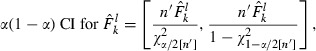
Confidence intervals on  , which can be used to calculate the CI of
  , were computed as follows (Waples 1989; Sokal and Rohlf 1995; Luikart et al. 1999):
 |
(3) |
where n′ is the number of independent alleles given by:
| (4) |
where Ki is the number of alleles of locus K.
We also studied a more recent version of a temporal based method, MLNE (Wang 2001; Wang and Whitlock 2003) which is based on likelihood estimation of effective population size. The number of cases studied was limited to only two bottleneck scenarios as the computational cost makes an exhaustive evaluation expensive.
The coefficient of variation (CV) is commonly used as a measure of precision and it is useful to compare results with theoretical expectations as these expectations hold for equilibrium. The CV for  based on LD is (Hill 1981; Waples and Do 2010):
| (5) |
where n is:
 |
(6) |
The CV provides a theoretical insight on other potential sources of lack of precision of the estimator: number of alleles and sample size are also expected to influence the precision of the estimator and most previous simulation studies of equilibrium report behaviours in line with theory. It is therefore important to investigate if qualitative and quantitative results hold for bottleneck cases.
The CV of the temporal estimator was presented in Pollak (1983):
| (7) |
where t is the time number of generations betweens samples and S is the sample size. The temporal based estimator has another expected source of imprecision: the temporal distance between samples.
We evaluated performance of both methods from three different perspectives:
Detection of a decline from the prebottleneck effective population size, for example to detect if the Ne (point estimate) is below 0.8 × N1. This is similar to bottleneck tests (e.g. Cornuet and Luikart (1996), as we are not concerned with the ability to approximate N2, only to detect if the population size decreased. The value chosen is arbitrary, but close to, and a function of N1.
Approximation of an effective population size that has declined closer to N2 than to N1. Here we try to understand if, adding to the previous ability to detect a decline, an estimator (point estimate) can approach the new effective size. For instance if there is a bottleneck of N1 = 600 to N2 = 50, we want to study the ability of estimators’ point estimate to be below 75, which is 50% above N2. This quantifies the ability to detect a change in Ne, but will not distinguish between an unbiased estimate of N2 and downward bias one.
Estimation of N2 with low bias and high precision and reliable confidence intervals. Most studies of equilibrium scenarios (stable population size) are of bias and precision and thus most comparable with this third perspective [e.g. England et al. (2006) and Wang and Whitlock (2003)].
The three perspectives above are presented as they might be useful in different situations: a practical research question might need only to detect that a population is declining (detection perspective) or it might require that a certain conservation threshold (e.g. Ne < 100) has been passed (approximation perspective) or, still, a precise and unbiased estimation of population size (estimation perspective). The first two perspectives are not applicable in equilibrium settings, but provide insights needed for practical conservation applications.
Methods for detection of population decline are reliable if, when there is no decline, the method does not erroneously suggest one (type I error). This effect is especially important with Ne estimators as their variance is known to increase with increasing real Ne. As such we also assess how often each estimator to detect a decline when there is none (false positive rate).
When characterizing the distribution of  across simulations, we use mainly box plots. Box plots show the median, 25th and 75th percentiles, the lowest datum within 1.5 of the lower quartile and the highest datum within 1.5 of the quartile range. Other measures like for example mean squared error, can be calculated from the Supporting Information (statistics from simulations).
We supply, as Supporting Information, the distribution of Ne estimates (point, upper and lower CI) according to the boundaries specified in the perspectives above (i.e. the percentage of estimations which fall above N1, 0.8N1, 1.5N2, 0.5N2 or below 0.5N2 for all scenarios studied for the first five generations following the population decline. We also supply a set of standard population genetics statistics for (Fst, expected heterozygosity and allelic richness) starting from the generation before the bottleneck up to 50 generations after. This material can be loaded in standard spreadsheet software for further analysis. Furthermore, we also include an extensive number of charts covering all statistical estimators for all scenarios studied. Supporting Information is made available on http://popgen.eu/ms/ne.
Results
With a fixed initial effective population size (N1) of 600 and a population decline to an N2 of 50, we could detect a reduction of  from the original N1 (detection perspective) after only one generation in 80% or more cases for each method when sampling just 25 individuals and 20 microsatellite loci. For an N2 of 100 the temporal method detected the decline only after a few generations or by using more samples or loci, while the LD based method still immediately detects a decline with just 25 individuals and loci. If N2 only drops to 200, the LD method will have still have power above 80% with 20 loci and 50 individuals at the first generation after the decline. Generally, the ability to detect a decline decreases for higher N2 for both estimators as expected from the CV (Waples and Do 2010) of both estimators.
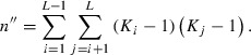
Both methods were able to approximate N2 (i.e. compute an estimation below 1.5N2) at generation two with a severe bottleneck of N2 = 50 if 50 individuals were sampled. However, the temporal method never had power above 80% for less severe bottlenecks (N2 = 100) in the first two generations. The power to detect an Ne < 1.5N2 (approximation perspective) is presented in Fig. 1.
Figure 1.
Power to detect that the effective population size (point estimate) is below 150%N2. The linkage disequilibrium (LD) based method is shown as a solid line and the temporal method with a dashed line. The horizontal dotted line is the 80% power threshold. Each column comprises a different N2 (50, 100, 200). The first row depicts 25 individuals and 20 loci; the second row 25 individuals and 40 loci; the third 50 individuals and 20 loci; the fourth 50 individuals and 40 loci.
As theoretically expected, power for early detection of a decline increases if more individuals are used. However, the following deviations from expectations (Waples 1989; Waples and Do 2010) are observed and further investigated in the discussion:
For the temporal method and for an N2 of 200, power decreased slightly with more samples.
Increasing the number of individuals sampled is more beneficial for both methods than increasing the number of loci. This effect is more noticeable with the LD method.
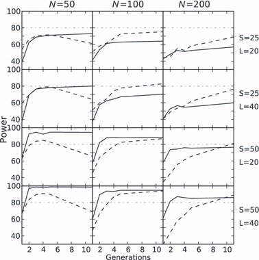
For the estimation perspective (i.e. low bias and small confidence intervals; see Methods), our bias and precision analysis showed that the temporal method has lower precision and, with larger N2, higher bias upwards than the LD method. With a very low number of individuals, the LD method is biased upwards (consistent with England et al. In press) and less precise than the temporal method in line with the effect presented above (Fig. 2).
Figure 2.
Boxplot charts of both the linkage disequilibrium (LD) and temporal point estimates up to six generations after a bottleneck with N1 = 600. The top chart reports a N2 = 50, and the bottom chart a N2 = 200. Different sampling strategies are shown on each column. On each chart, the top row depicts the LD method while the bottom row is the temporal method.
The MLNE did not perform better than the original moments-based temporal method. We used MLNE with two bottleneck scenarios (N2 of 50 and 200) and a sampling strategy using only two time points, MLNE never provided a reliable estimation even for large sample of 50 individuals and 40 loci. MLNE results were only usable with three samples in time but estimates were generally above N2 in concordance with Wang (2001) which also reports over-estimation of Ne in nonequilibrium scenarios (further details and an estimation perspective with MLNE are presented in the Supporting Information).
In order to understand the relative benefit of increasing the number of loci versus increasing the sample size, we simulated bottlenecks with an N1 = 300 and a N2 = 50 using two radically different sampling strategies: One maximizing the number of individuals (i.e. using a sample size equal to N2) but using only 10 loci and another using 50 loci but only 10 individuals. The scenario with five times more individuals than loci gave higher precision in both methods. This effect was more pronounced with the LD method as both bias and precision are affected during all the initial five generations (Fig. 3). The temporal method is mainly affected in precision, and only in the two initial generations for the scenario studied.
Figure 3.
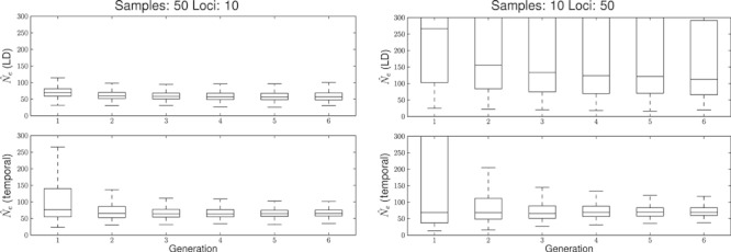
Boxplot of the  during the first five generations of a bottleneck from N1 = 300 to N2 = 50. The left column depicts a sample size of 50 and 10 loci and the right column 10 individuals and 50 loci. Top row is the linkage disequilibrium (LD) method and bottom row, the temporal method.
We also studied the behaviour of confidence intervals for both estimators. The upper confidence interval of the temporal method is often far higher than the initial population size during the initial bottleneck generations in most scenarios. This effect rarely occurs with the LD method: only on the very first generation and for high values of N2 (Fig. 4).
Figure 4.
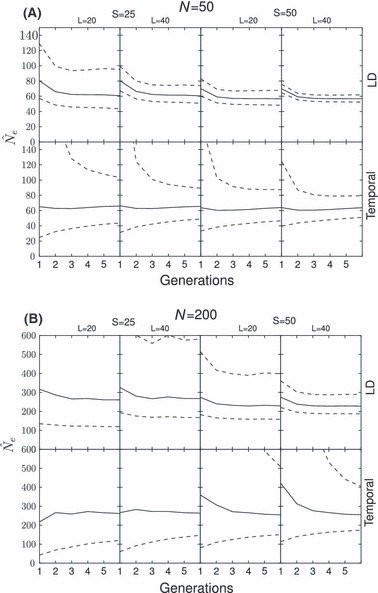
Harmonic mean of  (solid line) and 95% confidence intervals of 1200 postbottleneck replicates (dashed lines) for both methods for two bottleneck scenarios and four sampling strategies all with N1 = 600. The first chart reports a N2 = 50 and the second a N2 = 100. Different sampling strategies are shown on each panel from left to right: 25 individuals and 20 loci on the first, increasing to 40 on the second; the third shows 50 individuals and 20 loci increasing to 40 loci on the far right.
The usefulness of any estimator to detect a decline can be jeopardized by false positives, that is detection of a reduction in Ne when none occurred. We assessed the false positive rate for both estimators, that is with a true Ne of 600 (Fig. 5). The LD-based method lower quartile of estimates was always above 400, whereas the lower quartile of point estimates for the temporal method approaches 200 when the sample size is only 25 individuals. For a sample size of 50 the LD method point estimates were normally above 500 whereas the temporal method point estimates were occasionally only approximately 100 even though the true Ne was 600.
Figure 5.
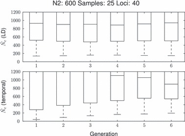
Boxplot of the distribution of point estimates for both estimators under equilibrium (N = 600) with 25 samples and 40 loci zooming in the area relevant for type I error detection. Estimates are biased high because the noise from sampling is often greater than the signal from drift or the number of parents.
We also studied how the prebottleneck size (N1) affects the behaviour of the estimators. We simulated bottlenecks with different initial population sizes (initial N1 = 1200, 600, 400, 300, 200 and final N2 = 50, Supporting Information). The LD method was little influenced by initial size, but the temporal method accuracy and precision decreased as N1 decreased. This effect was mostly visible on the first generation after the decline, and disappears shortly after. This means that, adding to type I errors which make methods less reliable to high N1, the temporal method also has precision problems with a lower N1.
We also quantified precision for bi-allelic markers (i.e. SNPs). Using 10 and 40 microsatellites and 40 and 100 SNPs a comparison among the distributions of the point estimates reveals results consistent with theoretical expectations (Fig. 6). As an example, 10 microsatellite loci gave slightly higher precision than 40 SNPs: as the median allelic richness for the microsatellite scenarios after the bottleneck is six (Supporting Information) the number of degrees of freedom (i.e. approximately the number of independent alleles) of the 40 SNPs scenario is smaller (20) than the 10 microsatellite scenario (50). The bias with SNPs is slightly lower probably because rare allele effects occurred less with bi-allelic markers we simulated. Type I errors also behave as expected, which for the sampling strategies shown and with equilibrium scenarios, there is not enough precision to differentiate between a type I error and a real decline, again making type I errors a fundamental consideration.
Figure 6.
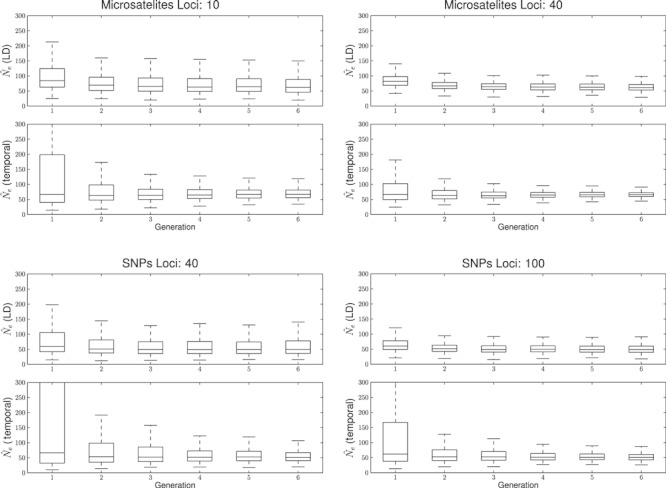
Boxplot of the  of both estimators during the first five generations of a bottleneck from 600 to 50 with a fixed sample size of 25. The top row depicts single nucleotide polymorphisms (SNPs), left 40 loci and right 100 loci. The bottom row depicts microsatellites, left 10 loci and right 40 loci.
We also quantified the influence of mutation rate on the ability to estimate Ne. The number of new mutations is negligible in small populations over 1–10 generations even with high mutation rates. As an example, for an Ne of 100 and a relatively high mutation rate of 0.001 the expected number of new mutations per generation per locus would be 0.2 (2 × Neμ). Simulation results show negligible effect (Supporting Information).
Discussion
Our results show that early detection and reliable size-estimation of population declines is increasingly possible using genetic monitoring and estimators of effective population size. Early detection is important as it allows for rapid management actions to avoid irreversible loss of genetic variation and increased risk of extinction due to genetic and demographic factors. Reliable estimation of Ne and the change in Ne is crucial in conservation biology but also in studies of evolution and ecology, for example to quantify bottleneck size associated with founder events or colonization of new environments.
LD method
The one-sample LD method generally outperformed the two-sample temporal method by allowing earlier detection of less severe population declines (N2 > 100) when using sample sizes of loci and individuals typical of studies today. Nonetheless, if the number of individuals sampled is low (≤25), the temporal method might be a better option, especially if multiple generations pass between temporal samples. Both methods were able to approximate the Nc of a bottlenecked population fairly quickly especially for Ne below 200, in most cases in less than three generations after the decline event. The generation number after the bottleneck might alter the relative performance of the estimators in a qualitatively meaningful way (e.g. bias is in an opposite direction for each estimator immediately after the bottleneck versus several generations after). Here, we are concerned with early detection, thus we note that some conclusions here might not hold if the generation gap is above 5–10 generations, which we did not study.
Temporal method
Experimental design (e.g. for a monitoring program) is more complex in the temporal method. Having two samples that are close temporally can yield relatively low precision (Wang and Whitlock 2003) while having two samples that are separated by many generations, biases the estimate up-ward (Richards and Leberg 1996; Luikart et al. 1999). This effect is easier to control in equilibrium scenarios as the underlying assumption of equilibrium would allow for some calibration of the distance between samples. But in nonequilibrium scenarios the uncertainty of a possible decline event between samples makes calibration less obvious.
For the temporal method and large N2, power declines as more individuals are sampled. This counter intuitive result can be attributed to two simultaneous causes: (i) Sampling more individuals raises the probability of increasing the number of rare alleles detected. Rare alleles are known to bias upward the temporal method (Turner et al. 2001), while the LD-based method includes an explicit correction (Waples and Gaggiotti 2006). (ii) On the other hand, a smaller decline (higher N2) will purge rare alleles more slowly. The precision of the temporal method is increasing with the number individuals sampled, but it is increasing towards an upward bias result, whereas the power definition used (relevant for the detection of a population decline) is concerned with detecting a value lower than a certain threshold. A correction to the temporal method (Jorde and Ryman 2007) to deal with upward bias does exist, but it is known to have a larger standard deviation than the original method (which is already large for the initial generations after the decline).
The MLNE method did not provide any improvement with only two sample time points. If more time points are available then MLNE might provide more reliable results, but in a context of early and timely estimation of a population decline this requirement for extra data might lower the usefulness of the method. Further research in MLNE is impaired by its computational cost (a study of the MLNE cost is available in the Supporting Information).
Confidence intervals for the LD method are generally much tighter than the temporal method even after the first 3–5 generations. While the interpretation of confidence intervals for both methods is not always straightforward [an exhaustive discussion can be seen in (Waples and Do 2010)] and its relevance is open to discussion, it is clear that there is a qualitative difference between estimators for early detection: The upper confidence interval for the temporal method often includes very high values, this is mainly caused by the known behaviour of the estimator to have poor precision for samples with only a few generations between samples.
Equations 1 and 2 show that the reference (i.e. before decline) and current (i.e. after decline) time are commutative in the temporal method. Our results show that the temporal method, when using a sample from before the bottleneck and another for after, tends towards the lowest value. This fortunate effect is fundamental in order to use the temporal approach to detect a decline. If the method did not approximate the lowest value then the first reference sample that could be used was one immediately after the bottleneck, therefore delaying any estimation of a decline.
Effect of prebottleneck size
The temporal method is also sensitive to the prebottleneck size for the estimation of Ne after decline. The more similar the size of the population before (N1) and after (N2) the decline the worse the temporal estimator performs. This has implications for the feasibility of genetic monitoring studies based on the temporal method: on one hand, as the prebottleneck size increases, the type I error also increases, on the other hand the closer N1 is to Ne, the larger the type II error (i.e. failure to detect a decline). Therefore, while the LD method is only sensitive to large prebottleneck sizes, the temporal method is also sensitive to the relationship between pre- and post-Ne. Experimental design (monitoring) with the temporal method could be more complex because the effect is more noticeable for relevant values of Ne and the small sample sizes common in conservation genetics scenarios. This effect tends to disappear soon after the bottleneck, so it will depend on the specific case to determine if very early detection is needed or not as that will have implications in the applicability of the temporal method.
Importance of number of samples
When trying to detect population declines, adding more individuals appears more beneficial than adding more loci, especially for the LD method. While previous studies (Waples 1989; Waples and Do 2010) have suggested that, for equilibrium scenarios, adding more loci is roughly interchangeable with adding more individuals, that is not the case when precise early detection of population decline is needed. This effect is unfortunate given that the ability to genotype more markers is fast increasing while sampling many individuals can be difficult for populations of conservation concern. When determining the feasibility of genetic monitoring strategies, researchers should be especially careful in determining if sampling of enough individuals at any point in time is feasible. As the temporal method is often less prone to this effect – in fact it might not even be affected at all as empirical analysis suggest (Palstra and Ruzzante 2008) – if the ability to sample many individuals is low then the temporal method might be a better option. Further research is needed to formally characterize both estimators after a bottleneck, especially trying to understand how past history and current state influence precision and bias and to why the benefits of adding loci and samples are not similar to nonequilibrium scenarios.
Single nucleotide polymorphisms
As expected, SNPs provide less precision and accuracy (per locus) than microsatellites for estimation of Ne. Both methods depend on the number of independent alleles for a precise estimate in equilibrium populations, therefore the expectation is that using bi-allelic loci will provide lower precision compared to microsatellites; this also appears true for declining populations. Nonetheless, the bias with SNPs is slightly lower (probably because rare allele effects occur less with bi-allelic markers we simulated). Again, the rate of false positives becomes a fundamental consideration, impairing the ability to detect a decline (Supporting Information). Further research is needed to quantify effects of different numbers of alleles (e.g. replacing microsatellites with a higher number of SNPs) in nonequilibrium scenarios, especially as we have demonstrated that, contrary to equilibrium scenarios, increasing the number of loci and sample size do not equally improve precision and accuracy.
Assumptions
Three assumptions of our work deserve mention and future research. First, future research is needed to quantify the effects of violating the assumption of no migration, and to develop methods to jointly estimate Ne and migration that is generalizable over a range of metapopulation models. Methods have been proposed (Vitalis and Couvet 2001; Wang and Whitlock 2003) to jointly estimate migration and Ne but have not been thoroughly evaluated or are not highly generalizable (e.g. beyond equilibrium populations or continent-island metapopulation systems). Another important assumption is nonoverlapping generations. Most methods has not been extended to (or evaluated for) species with overlapping generations or age structure [but see Jorde and Ryman (1995) and Waples and Yokota (2007)]. A third important assumption that requires thorough evaluation is mating system or behaviour which could bias the LD method, for example if a mating system generates LD. Further research is needed to assess the importance of the issues presented above before applying the Ne estimators to scenarios mentioned above.
Type I error rate
False positives (i.e. type I errors) are a concern when designing a study or monitoring program to detect a population decline, because false positives can lead to the waste of conservation resources on populations not actually declining. The temporal method is arguably more prone to false positive detection than the LD method. The need for more individuals or markers can sometimes be justified not by bias and precision in estimating postbottleneck sizes but mostly by the need to avoid false positives, as Ne estimators are less precise with the larger, predecline, real Ne. This false positive effect might be less important in some conservation cases where the original population is known to be very low even prebottleneck. As in some conservation management cases the consequences of acting when there is no need is normally much smaller than the cost of not acting when there is a need (i.e. type II error), for example to avoid extinction, a somewhat high probability of false positives might, in any case, be acceptable although this will vary from case to case.
Other methods
Several other methods to estimate Ne have been proposed (Nomura 2008; Tallmon et al. 2008) and a comprehensive comparison of performance would be useful. Likelihood based methods (like MLNE) are expected to be computationally intensive making comprehensive studies difficult as the computational cost to conduct a large number of simulations and posterior evaluation could be prohibitive. This questions the practical applicability of computationally intensive methods as comprehensive evaluations of performance and reliability will require vast amount of computational resources. Thus evaluation of performance often will be, in practice, limited to a small number of scenarios. Approximate Bayesian and summary statistic methods including multiple summary statistics (e.g. both temporal F and LD) could greatly improve precision and accuracy of Ne estimators (Tallmon et al. 2008; Luikart et al. 2010), especially as large population genomic data sets become common making likelihood-based methods even computationally demanding to evaluate (Luikart et al. 2003).
Conclusion
Early detection of population declines is increasingly feasible with the use of genetic monitoring based on effective population size estimators. If the number of samples is sufficiently high, LD based method is arguably more powerful and better suited for monitoring to detect declines because it is less prone to type I errors, has tighter confidence intervals, and is more flexible with regards to designing different experimental design strategies. Nonetheless it is important to further research the behaviour of both estimators under an even broader set of realistic scenarios, for example with age structure or migration, and to understand if variations of the temporal method (Jorde and Ryman 1996) or LDNe allow for earlier and more precise estimation of effective population size in decline populations. Both methods along with others (e.g. loss of alleles) should often be used when monitoring in order to gain a better understanding of the causes, consequences and severity of population declines (Luikart et al. 1999).
As the precision of both estimators requires the true effective population size to be relatively small, their use is currently limited to scenarios in conservation biology and perhaps studies of the ecology and evolution in small populations. For instance, they cannot be used to conduct reliable genetic monitoring when the effective size remains larger than approximately 500–1000 unless perhaps hundreds of loci and individuals are sampled and/or improved estimators are developed.
Combining simulation evaluations of new statistical methods and increasing numbers of DNA markers makes management and genetic monitoring increasingly useful for early detection of population declines, even with noninvasive sampling of elusive or secretive species. This results are encouraging and contribute to the excitement and promise of using genetics in conservation and management.
Acknowledgments
We thank R. Waples for helpful advice and sharing computer code for the LDNe program, and P.R. England, D.A. Tallmon, and F.W. Allendorf for helpful discussions. Finally, we thank the two anonymous reviewers for their insightful comments.
T.A. was supported by research grant SFRH/BD/30834/2006 from Fundação para a Ciência e Tecnologia (FCT), Portugal. G.L. was partially supported by the Luso-American Foundation, the Walton Family Foundation, U.S. National Science Foundation (Grant DEB 074218) and CIBIO. A.P.F. was supported by an Ángeles Alvariño fellowship from Xunta de Galicia (Spain). This project was supported by grant PTDC/BIA-BDE/65625/2006 also from FCT.
Supporting Information
Additional Supporting Information is provided on our website at http://popgen.eu/ms/ne/
Please note: Wiley-Blackwell is not responsible for the content or functionality of any supporting materials supplied by the authors. Any queries should be directed to the corresponding author for the article.
Literature cited
- Charlesworth B. Fundamental concepts in genetics: effective population size and patterns of molecular evolution and variation. Nature Reviews Genetics. 2009;10:195–205. doi: 10.1038/nrg2526. [DOI] [PubMed] [Google Scholar]
- Cock PJA, Antao T, Chang JT, Chapman BA, Cox CJ, Dalke A, Friedberg I, et al. Biopython: freely available python tools for computational molecular biology and bioinformatics. Bioinformatics. 2009;25:1422–1423. doi: 10.1093/bioinformatics/btp163. [DOI] [PMC free article] [PubMed] [Google Scholar]
- Cornuet JM, Luikart G. Description and power analysis of two tests for detecting recent population bottlenecks from allele frequency data. Genetics. 1996;144:2001–2014. doi: 10.1093/genetics/144.4.2001. [DOI] [PMC free article] [PubMed] [Google Scholar]
- Crow JF, Kimura M. Introduction to Population Genetics Theory. New York: Harper & Row Publishers; 1970. [Google Scholar]
- Ellegren H. Microsatellites: simple sequences with complex evolution. Nature Reviews Genetics. 2004;5:435–445. doi: 10.1038/nrg1348. [DOI] [PubMed] [Google Scholar]
- England P, Cornuet J-M, Berthier P, Tallmon D, Luikart G. Estimating effective population size from linkage disequilibrium: severe bias in small samples. Conservation Genetics. 2006;7:303–308. [Google Scholar]
- England P, Luikart G, Waples R. Early detection of population fragmentation using linkage disequilibrium estimation of effective population size. Conservation Genetics. In press. In press. [Google Scholar]
- Frankham R. Genetics and extinction. Biological Conservation. 2005;126:131–140. [Google Scholar]
- Hill WG. Estimation of effective population size from data on linkage disequilibrium. Genetics Research. 1981;38:209–216. [Google Scholar]
- Jorde PE, Ryman N. Temporal allele frequency change and estimation of effective size in populations with overlapping generations. Genetics. 1995;139:1077–1090. doi: 10.1093/genetics/139.2.1077. [DOI] [PMC free article] [PubMed] [Google Scholar]
- Jorde PE, Ryman N. Demographic genetics of brown trout (Salmo trutta) and estimation of effective population size from temporal change of allele frequencies. Genetics. 1996;143:1369–1381. doi: 10.1093/genetics/143.3.1369. [DOI] [PMC free article] [PubMed] [Google Scholar]
- Jorde PE, Ryman N. Unbiased estimator for genetic drift and effective population size. Genetics. 2007;177:927–935. doi: 10.1534/genetics.107.075481. [DOI] [PMC free article] [PubMed] [Google Scholar]
- Krimbas CB, Tsakas S. The genetics of Dacus oleae. V. changes of esterase polymorphism in a natural population following insecticide control-selection or drift. Evolution. 1971;25:454–460. doi: 10.1111/j.1558-5646.1971.tb01904.x. [DOI] [PubMed] [Google Scholar]
- Leberg P. Genetic approaches for estimating the effective size of populations. Journal of Wildlife Management. 2005;69:1385–1399. [Google Scholar]
- Luikart G, Cornuet J-M, Allendorf FW. Temporal changes in allele frequencies provide estimates of population bottleneck size. Conservation Biology. 1999;13:523–530. [Google Scholar]
- Luikart G, England PR, Tallmon D, Jordan S, Taberlet P. The power and promise of population genomics: from genotyping to genome typing. Nature Reviews Genetics. 2003;4:981–994. doi: 10.1038/nrg1226. [DOI] [PubMed] [Google Scholar]
- Luikart G, Ryman N, Tallmon D, Schwartz MK, Allendorf FW. Estimating census and effective population sizes: increasing usefulness of genetic methods. Conservation Genetics. 2010;11:355–373. [Google Scholar]
- Nei M, Tajima F. Genetic drift and estimation of effective population size. Genetics. 1981;98:625–640. doi: 10.1093/genetics/98.3.625. [DOI] [PMC free article] [PubMed] [Google Scholar]
- Nomura T. Estimation of effective number of breeders from molecular coancestry of single cohort sample. Evolutionary Applications. 2008;1:462–474. doi: 10.1111/j.1752-4571.2008.00015.x. [DOI] [PMC free article] [PubMed] [Google Scholar]
- Nunney L, Elam DR. Estimating the effective population size of conserved populations. Conservation Biology. 1994;8:175–184. [Google Scholar]
- Palstra FP, Ruzzante DE. Genetic estimates of contemporary effective population size: what can they tell us about the importance of genetic stochasticity for wild population persistence. Molecular Ecology. 2008;17:3428–3447. doi: 10.1111/j.1365-294x.2008.03842.x. [DOI] [PubMed] [Google Scholar]
- Peng B, Kimmel M. simuPOP: a forward-time population genetics simulation environment. Bioinformatics. 2005;21:3686–3687. doi: 10.1093/bioinformatics/bti584. [DOI] [PubMed] [Google Scholar]
- Pollak E. A new method for estimating the effective population size from allele frequency changes. Genetics. 1983;104:531–548. doi: 10.1093/genetics/104.3.531. [DOI] [PMC free article] [PubMed] [Google Scholar]
- Richards C, Leberg PL. Temporal changes in allele frequencies and a population's history of severe bottlenecks. Conservation Biology. 1996;10:832–839. [Google Scholar]
- Rousset F. genepop’007: a complete re-implementation of the genepop software for windows and linux. Molecular Ecology Resources. 2008;8:103–106. doi: 10.1111/j.1471-8286.2007.01931.x. [DOI] [PubMed] [Google Scholar]
- Schug MD, Mackay TF, Aquadro CF. Low mutation rates of microsatellite loci in drosophila melanogaster. Nature Genetics. 1997;15:99–102. doi: 10.1038/ng0197-99. [DOI] [PubMed] [Google Scholar]
- Sokal RR, Rohlf FJ. Biometry. New York: W. H. Freeman and Co; 1995. [Google Scholar]
- Tallmon DA, Koyuk A, Luikart G, Beaumont MA. onesamp: a program to estimate effective population size using approximate bayesian computation. Molecular Ecology Notes. 2008;8:299–301. doi: 10.1111/j.1471-8286.2007.01997.x. [DOI] [PubMed] [Google Scholar]
- Turner T, Salter L, Gold J. Temporal-method estimates of ne from highly polymorphic loci. Conservation Genetics. 2001;2:297–308. [Google Scholar]
- Vitalis R, Couvet D. Estimation of effective population size and migration rate from one- and two-locus identity measures. Genetics. 2001;157:911–925. doi: 10.1093/genetics/157.2.911. [DOI] [PMC free article] [PubMed] [Google Scholar]
- Wang J. A pseudo-likelihood method for estimating effective population size from temporally spaced samples. Genetics Research. 2001;78:243–257. doi: 10.1017/s0016672301005286. [DOI] [PubMed] [Google Scholar]
- Wang J, Whitlock MC. Estimating effective population size and migration rates from genetic samples over space and time. Genetics. 2003;163:429–446. doi: 10.1093/genetics/163.1.429. [DOI] [PMC free article] [PubMed] [Google Scholar]
- Waples R, Gaggiotti O. What is a population?: an empirical evaluation of some genetic methods for identifying the number of gene pools and their degree of connectivity. Molecular ecology. 2006;15:1419–1439. doi: 10.1111/j.1365-294X.2006.02890.x. 10.1111/j.1365-294X.2006.02890.x. [DOI] [PubMed] [Google Scholar]
- Waples RS. A generalized approach for estimating effective population size from temporal changes in allele frequency. Genetics. 1989;121:379–391. doi: 10.1093/genetics/121.2.379. [DOI] [PMC free article] [PubMed] [Google Scholar]
- Waples RS. A bias correction for estimates of effective population size based on linkage disequilibrium at unlinked gene loci*. Conservation Genetics. 2006;7:167–184. [Google Scholar]
- Waples RS, Do C. ldne: a program for estimating effective population size from data on linkage disequilibrium. Molecular Ecology Resources. 2008;8:753–756. doi: 10.1111/j.1755-0998.2007.02061.x. [DOI] [PubMed] [Google Scholar]
- Waples RS, Do C. Linkage disequilibrium estimates of contemporary Ne using highly variable genetic markers: a largely untapped resource for applied conservation and evolution. Evolutionary Applications. 2010;3:244–262. doi: 10.1111/j.1752-4571.2009.00104.x. [DOI] [PMC free article] [PubMed] [Google Scholar]
- Waples RS, Yokota M. Temporal estimates of effective population size in species with overlapping generations. Genetics. 2007;175:219–233. doi: 10.1534/genetics.106.065300. [DOI] [PMC free article] [PubMed] [Google Scholar]
- Weir BS, Cockerham CC. Estimating f-statistics for the analysis of population structure. Evolution. 1984;38:1358–1370. doi: 10.1111/j.1558-5646.1984.tb05657.x. [DOI] [PubMed] [Google Scholar]
Associated Data
This section collects any data citations, data availability statements, or supplementary materials included in this article.