Statistical Deconvolution for Superresolution Fluorescence Microscopy

Abstract

Superresolution microscopy techniques based on the sequential activation of fluorophores can achieve image resolution of ∼10 nm but require a sparse distribution of simultaneously activated fluorophores in the field of view. Image analysis procedures for this approach typically discard data from crowded molecules with overlapping images, wasting valuable image information that is only partly degraded by overlap. A data analysis method that exploits all available fluorescence data, regardless of overlap, could increase the number of molecules processed per frame and thereby accelerate superresolution imaging speed, enabling the study of fast, dynamic biological processes. Here, we present a computational method, referred to as deconvolution-STORM (deconSTORM), which uses iterative image deconvolution in place of single- or multiemitter localization to estimate the sample. DeconSTORM approximates the maximum likelihood sample estimate under a realistic statistical model of fluorescence microscopy movies comprising numerous frames. The model incorporates Poisson-distributed photon-detection noise, the sparse spatial distribution of activated fluorophores, and temporal correlations between consecutive movie frames arising from intermittent fluorophore activation. We first quantitatively validated this approach with simulated fluorescence data and showed that deconSTORM accurately estimates superresolution images even at high densities of activated fluorophores where analysis by single- or multiemitter localization methods fails. We then applied the method to experimental data of cellular structures and demonstrated that deconSTORM enables an approximately fivefold or greater increase in imaging speed by allowing a higher density of activated fluorophores/frame.

Introduction

Superresolution fluorescence microscopy techniques based on single-molecule localization achieve subdiffraction-limit resolution by stochastically activating individual fluorophores and computationally determining the fluorophore positions (1). For example, stochastic optical reconstruction microscopy (STORM) and (fluorescence) photoactivated localization microscopy ((F)PALM) take advantage of photoswitchable probes to temporally separate the spatially overlapping images of individual molecules (2–4). At any instant during the image acquisition, only a sparse subset of the fluorescent probes in the field of view is activated, such that the positions of the probes can be precisely determined from their individual images. A superresolution image can then be reconstructed by accumulating numerous fluorophore positions over time. Computing the fluorophore coordinates from their corresponding images is thus central to these superresolution techniques. However, analysis methods that accomplish this task typically rely on simplistic assumptions about image acquisition that limit the speed and efficiency of imaging. For example, most current methods assume that fluorophore localization requires isolated images of individual fluorophores (2–6), since overlapping images carry reduced information (7). These methods therefore discard data from nearby fluorophores with overlapping images, limiting the density of fluorophores that can be localized per frame and necessitating thousands to tens of thousands of frames to build up enough points to estimate an image. Yet image overlap between molecules only partially degrades the localization precision (8), suggesting the possibility of localizing a higher density of fluorophores/frame and thus increasing the overall imaging speed.

Indeed, several methods have been recently developed to take advantage of information from such high-density samples with overlapping single-molecule images, either by comparing subsequent frames, by directly fitting the overlapping images of multiple emitters, or by using high-order correlations in the fluorescence data. For example, super-resolution imaging can be accomplished by subtracting subsequent movie frames to reveal the transient blinking or bleaching of isolated individual fluorophores (9,10). This elegant approach substantially extends the range of fluorophores available for localization-based superresolution imaging. The imaging speed is, however, not substantially increased, because the subtracted images are still analyzed by single-emitter fitting and thus the number of localizations that can be detected per frame is similar to the other single-emitter localization based approaches. Localization precision may also be reduced for emitters that remain activated during a series of several frames, because only photons in the first and last frames of the series are used for localization. Simultaneously fitting overlapping images from multiple activated fluorophores can substantially shorten the imaging time (11–13), but this approach is computationally challenging due to the high-dimensional space of possible molecular configurations that could give rise to a given sequence of images. The computational time thus increases exponentially and the localization accuracy decreases with increasing density of simultaneously activated fluorophores. A Bayesian analysis has been developed to address this problem by taking advantage of the temporal correlations arising from fluorophore blinking and bleaching (13), though simplifying assumptions, such as Gaussian-distributed photon-detection noise, are invoked. Overall, localization of molecules becomes increasingly more difficult and less accurate as the density of simultaneously emitting fluorophores increases. Higher-order correlation analysis of the temporal fluctuations of individual pixels can also be used to analyze high-density samples and yield subdiffraction-limit images (14). This method, called superresolution optical fluctuation imaging (SOFI), can potentially achieve faster imaging speed than localization-based superresolution methods, but with a lower spatial resolution.

In this work, we developed an image-deconvolution-based method that can analyze multiframe fluorescence movies and obtain superresolution images without the need of localizing molecules. A microscope forms a far-field image of the sample that is blurred, or convolved, with the instrument's point spread function (PSF), the width of which is typically limited to ∼200 nm by the diffraction of light. Convolution is a linear operation that can be reversed by convolving with an appropriate sharpening filter, to recover the true sample. In practice, however, noise in the fluorescence data, such as Poisson-distributed photon shot noise, may be severely amplified by linear deconvolution procedures. This negates the benefit of image deconvolution and prevents the use of linear deconvolution for reconstructing image features substantially smaller than the diffraction limit. Here we develop a nonlinear deconvolution procedure that avoids noise amplification by using a realistic statistical model of fluorescence data from intermittently activated molecules and allows a superresolution image to be reconstructed from movies with a relatively high density of activated fluorophores/frame. This approach, referred to as deconvolution-STORM (deconSTORM), directly estimates a superresolution image (i.e., the intensity values at a discrete set of pixels more finely spaced than the original camera pixels), rather than a set of emitter locations. This method thus differs fundamentally from superresolution methods based on localization of individual molecules. Our validation studies using simulations and cellular data show that deconSTORM allows a substantial increase in the imaging speed compared to single-molecule-localization-based techniques.

Methods

Simulations and data analysis were carried out using custom code written in MATLAB (The MathWorks, Natick, MA). To allow other researchers to use the deconSTORM method, a MATLAB toolbox for implementing the method is available at http://zhuang.harvard.edu/software.html.

deconSTORM: a statistical deconvolution analysis method

Determining the best estimate of a sample's structure based on noisy fluorescence images is a statistical estimation problem. Our statistical model assumes that the true sample at time frame k is a positive semidefinite function, $i_k\left(x\right)$, representing the brightness of activated fluorophores at a discrete grid of locations, $x\in X$. The number of fluorescence photons detected at each camera pixel y, $N_k\left(y\right)$, is a Poisson-distributed random variable related to $i_k\left(x\right)$ by

$$P\left[\left\{N_k\left(y\right)\right\}|i_k\right]=\prod _{y\in Y}{e}^{-{\lambda }_k\left(y\right)}\frac{{\lambda }_k{\left(y\right)}^{N_k\left(y\right)}}{N_k\left(y\right)!}.$$ (1)

The grid of camera pixels, Y, is in general coarser than the superresolution sample grid, X. The expected intensity, ${\lambda }_k\left(y\right)$, is the sum of the background fluorescence intensity, b, and the convolution of the true image with the PSF, h:

$${\lambda }_k\left(y\right)=\sum _{x\in X}h\left(y-x\right)i_k\left(x\right)+b.$$ (2)

The PSF is normalized so that ${\sum }_{x\in X}h\left(y-x\right)=1$ for all y. We sought a method to approximate the maximum-likelihood image based on all available data, without explicitly estimating emitter locations. To do this, we adapted the iterative image deconvolution algorithm of Richardson and Lucy (RL), which converges to the maximum-likelihood estimate of a true image given blurred, noisy data with Poisson statistics (15–17).

RL deconvolution begins, at iteration $t=1$, with a uniform estimate of the image intensity at location x in frame k, ${\hat{i}}_k^{t=1}\left(x\right)=1$ (we use a circumflex to denote estimated quantities). The expected number of fluorescence photons at pixel y is ${\hat{N}}_k^t\left(y\right)={\sum }_{x\in X}h\left(y-x\right){\hat{i}}_k^t\left(x\right)+b$. We assume that h and b are known; these quantities can be calibrated, e.g., using data from sparsely distributed fluorophores whose individual images do not overlap. The discrepancy between the observed and expected number of photons is captured by the error ratio at each camera pixel, $e_k^t\left(y\right)\equiv N_k\left(y\right)/{\hat{N}}_k^t\left(y\right)$. RL deconvolution updates the sample estimate by multiplying by the convolution of this error ratio with the PSF,

$${\hat{i}}_k^{t+1}\left(x\right)={\hat{i}}_k^t\left(x\right)\sum _{y\in Y}h\left(x-y\right)e_k^t\left(y\right)/a\left(x\right).$$ (3)

Here, $a\left(x\right)\equiv {\sum }_{y\in Y}h\left(x-y\right)$ is a normalizing constant. This algorithm is an expectation-maximization (EM) procedure that is guaranteed to converge to the maximum-likelihood sample estimate (15–17), but the speed of convergence can be very slow.

It has been shown that the convergence of RL deconvolution may be accelerated by modifying the algorithm to incorporate statistical prior information about the distribution of pixel intensities (18,19). We therefore adapted the classic RL algorithm in two ways to incorporate realistic statistical features of the spatial and temporal distribution of stochastically activated fluorophores in a movie. First, each movie frame consists of images of relatively sparsely distributed fluorophores, because only a dilute set of fluorophores is activated. Here, we note that the word sparse does not imply that the images of activated fluorophores are all well isolated from each other, but instead means that these images are not sufficiently crowded to cover all areas in the field of view. Therefore, substantial overlap between images is allowed. A sparse prior distribution for the pixel intensities in the superresolution image is therefore appropriate and may improve the convergence speed of the RL algorithm. An exponential prior distribution of the form $P\left[\hat{i}\right]\propto \exp \left[-\gamma \hat{i}\right]$ promotes sparseness (20) and can be implemented by including a divisive factor in the RL update rule (18):

$${\hat{i}}_k^{t+1}\left(x\right)={\hat{i}}_k^t\left(x\right)\sum _{y}h\left(x-y\right)e^t\left(y\right)/\left(a\left(x\right)+\gamma \right).$$ (4)

We refer to this procedure as RL with constant prior, since the parameter γ is the same at every location and time frame.

Both of the above deconvolution procedures, RL (Eq. 3) and RL with constant prior (Eq. 4), treat each movie frame independently, ignoring temporal correlations between frames due to intermittent fluorophore activation and deactivation. Considering this temporal correlation could increase the accuracy in the estimated image. We next designed a deconSTORM deconvolution procedure to take into account the stochastic dynamics of emitter activation and deactivation to further improve the speed and accuracy of image estimation. We assume that each emitter switches between an activated (fluorescent) state and an off (dark) state according to a Markov process, with transition probabilities β (activation) and α (inactivation) in each frame; this is illustrated in Fig. 1, a and b. Each emitter's transitions are statistically independent of the other emitters' states. As with the PSF, h, and background intensity, b, we assume that β and α are known; these parameters are determined by the photophysics of the fluorophore, as well as the intensity of the activation laser, and they may be easily calibrated. The switching dynamics of individual fluorophores generate correlations that can be used to improve the sample estimate in a given frame by using information from other frames.

Figure 1.

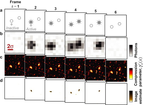
Schematic illustration of the deconSTORM algorithm for analyzing multiframe fluorescence movie data of intermittently activated fluorophores. (a) Simulation of a small field of view containing two nearby fluorophores. In this sequence of six frames, open and solid circles denote the off (dark) and activated (fluorescent) states, respectively. (b) Simulated fluorescence data for each frame; σ is the width parameter of the microscope's PSF, which is equal to the pixel spacing of the simulated fluorescence data. (c) The deconSTORM compression parameter, ${\gamma }_k^t\left(x\right)$, at pixel x and time frame k at iteration t = 500. (d) Estimated image for each movie frame after 500 iterations of deconSTORM deconvolution.

To do this, we reasoned that information from temporal correlations could be used to optimize the sparseness parameter, γ, at each location and time frame. We therefore assigned each location in each movie frame its own exponential prior distribution with parameter ${\gamma }_k^t\left(x\right)$, whose value is updated iteratively in parallel with the superresolution sample estimate, ${\hat{i}}_k^t\left(x\right)$ (Fig. 1 c). ${\gamma }_k^t\left(x\right)$ acts as a compression factor that biases the corresponding location's estimated intensity toward zero (Fig. 1 d). The compression factor at location x in frame k is based on a weighted average of the sample estimate at x in the full set of K movie frames, with higher weight given to the frames immediately before or after the current frame:

$${\gamma }_k^t\left(x\right)=\max \left\{-g\ln \left[\sum _{k^{\prime }=1}^K\left(\frac{{\alpha }^{|k-k^{\prime }|}}{2\left(1-\alpha \right)}+\frac{\beta }{K}\right){\hat{i}}_{k^{\prime }}^t\left(x\right)\right],0\right\}.$$ (5)

g is a gain parameter that controls the overall amount of compression; in practice, we found that a value of g = 1/256 provided an appropriate balance of compression and accuracy. The first term inside the logarithm in the update rule (Eq. 5) ensures that observation of intense fluorescence at a particular location in one movie frame reduces the compression factor at the same location in subsequent and preceding frames. Since an activated emitter remains active for 1/α frames on average, the influence of each frame on the compression parameter in other frames decays exponentially as a function of the time lag between them. The second term in Eq. 5 is motivated by the fact that an emitter detected in any time frame may be reactivated in any earlier or later frame with probability β. Both terms cause the compression factor to decay toward zero (i.e., no extra compression) in regions where the prior expectation of an activated emitter is high. In regions of the field of view with near-background fluorescence intensity throughout the data set, the value of the compression factor increases and the estimated image in these regions will be biased toward zero.

Table 1 summarizes the deconSTORM algorithm, as well as the classic RL deconvolution procedure and RL with constant prior.

Table 1.

Three deconvolution-based algorithms and glossary of notation

Variable name	Symbol	Variable name	Symbol
Detected fluorescence photons in frame k in pixel y	$N_k\left(y\right)$	Compression factor	${\gamma }_k^t\left(y\right)$
Background brightness	b	deconSTORM gain factor	g
PSF	$h\left(y\right)$	Total number of frames	K
Fluorophore inactivation probability/frame	α	Estimated image intensity after t iterations of deconvolution at location x for frame k	${\hat{i}}_k^t\left(x\right)$
Fluorophore activation probability/frame	β	Normalization of the PSF	$a\left(x\right)\equiv {\sum }_{y}h\left(x-y\right)$
Algorithm
1. Initialize the sample estimate	${\hat{i}}_k^1\left(x\right)=1$
2. For t = 1 to n:
2.1 Compute ratio of data to prediction	$e^t\left(y\right)=\frac{N_k\left(y\right)}{\sum _{x}h(y-x){\hat{i}}_k^t\left(x\right)+b}$
2.2 Compute sparseness parameter
i. RL	${\gamma }_k^t\left(x\right)=0$
ii. RL with constant prior	${\gamma }_k^t\left(x\right)=\gamma$
iii. deconSTORM	${\gamma }_k^t\left(x\right)=\max \left\{-g\log \left[\sum _{k^{\prime }=1}^K\left(\frac{{\alpha }^{|k-k^{\prime }|}}{2\left(1-\alpha \right)}+\frac{\beta }{K}\right){\hat{i}}_{k^{\prime }}^t\left(x\right)\right],0\right\}$
2.3 Update sample estimate	${\hat{i}}_k^{t+1}\left(x\right)={\hat{i}}_k^t\left(x\right)\sum _{y}h\left(x-y\right)e^t\left(y\right)/\left(a\left(x\right)+{\gamma }_k^t\left(x\right)\right)$

Three deconvolution-based algorithms are RL, RL with constant prior, and deconSTORM.

Simulated localization microscopy data sets

To validate our analysis method, we simulated multiframe fluorescence microscopy data sets in which only a subset of fluorophores was activated in each frame. All distances were expressed in units of σ, the width parameter of the optical PSF (defined below). Here, we choose σ ∼ 150 nm. The field of view was divided into an 8 × 8 grid of camera pixels, and the side length of each pixel was 1σ. The resulting field-of-view area was 64 σ², corresponding to several diffraction-limited regions. For each simulation, we created a sample consisting of M = 30 pointlike emitters whose x- and y-coordinates were randomly drawn from a uniform distribution on the interval, [0,8σ). These samples therefore have a uniform average fluorophore density. Each emitter had two states, an off state and an activated state, with transitions occurring independently with probability β and α for activation and inactivation, respectively. We set α = 1/2 for all simulations. β varied from ∼10⁻⁴, corresponding to a low average density of activated emitters, up to ∼0.1, producing extensive overlap between neighboring images of emitters. In the first movie frame of a simulated data set, each emitter was chosen to be in the activated state with probability P = β/(1 − α + β), the steady-state activation probability for an individual emitter. The density of simultaneously fluorescent emitters is thus ρ = PM/(8σ)², and the mean separation between activated emitters is $d=\sqrt{1/\rho }$.

To create a fair comparison among simulations with different activation rates, we reduced the number of movie frames, N, as the activated emitter density increased so that the total number of fluorescence photons collected from activated emitters is roughly the same: N ≈ 13/β.

The expected number of fluorescence photons at pixel j in time frame k was

$$i_k\left({\mathbf{r}}_j\right)=\sum _{l=1}^M{s}_{l,k}h\left({\mathbf{r}}_j-{\mathbf{r}}_l\right)+b,$$ (6)

where $s_{l,k}\in \left\{0,1\right\}$ defines the state (off or activated) of emitter l in frame k; the vector ${\mathbf{r}}_j$ is the position of the jth pixel; ${\mathbf{r}}_l$ is the position of the lth emitter; and the PSF is a periodic Gaussian function:

$$h\left({\mathbf{r}}_1-{\mathbf{r}}_2\right)=B\sum _{m_x,m_y=-\mathrm{\infty }}^{\mathrm{\infty }}\exp [-\frac{{\left(x_1-x_2+m_{x}8\sigma \right)}^2}{2{\sigma }^2}-\frac{{\left(y_1-y_2+m_{y}8\sigma \right)}^2}{2{\sigma }^2}].$$ (7)

The sum over m_x and m_y effectively creates periodic boundary conditions, eliminating effects due to the edges of the simulated field of view. The brightness parameter, B, was chosen so that ${\sum }_{k=1}^{64}h\left({\mathbf{r}}_k\right)=250$ photons/frame, whereas the mean background fluorescence intensity was b = 1 photon/pixel/frame. These parameter choices correspond to a relatively high signal/noise ratio, which should provide a best-case scenario for comparing both localization-based and deconvolution-based analysis methods. The simulated fluorescence data at each pixel were drawn from a Poisson distribution with mean $i_k\left({\mathbf{r}}_j\right)$. We did not include noise introduced by readout of the camera pixels, which is typically small compared with the fundamental fluctuations due to photon shot noise.

Deconvolution analysis

For analysis of both simulated and experimental fluorescence movie data sets, we implemented three image-deconvolution algorithms: RL, RL with constant prior, and deconSTORM. The size of simulated images was 8σ × 8σ, and experimental data were 16σ × 16σ. The three deconvolution algorithms are summarized in Table 1. We estimated images with resolution eightfold finer than that of the original camera pixels, so that the width of each superresolution pixel is $\sigma /8$.

Comparison with single- and multiemitter localization procedures

We compared the performance of the three deconvolution methods (RL, RL with constant prior, and deconSTORM) with two localization-based procedures that fit the images to determine the positions of individual emitters. For single-emitter fitting, we used nonlinear optimization to find the maximum-likelihood estimate of each emitter's location (6). We sought to give this procedure the best possible chance of success and thus establish an upper bound on its performance in practice. For this purpose, in our studies of simulated data, we initialized the fit using each emitter's true location parameters, even though these would be unavailable in analyzing experimental data. For isolated emitters, this procedure should achieve the minimum localization-error variance as defined by the Cramér-Rao lower bound (6). However, when images of nearby emitters overlap, the localization accuracy may be substantially worse. We implemented maximum-likelihood fitting using a constrained nonlinear multivariable optimization interior point algorithm (MATLAB routine fmincon). For each emitter, the algorithm estimated four parameters (x,y coordinates, amplitude, and background intensity). The fitted x,y coordinates were constrained to lie within ±4σ of the true location.

For multiemitter fitting we used DAOSTORM, a previously reported software package (12). Parameters for this analysis were set according to instructions in the reference manual provided with the software.

Quantitative analysis of image reconstruction quality

Quantitative measures that have been used in previous studies to evaluate the performance of single- and multiemitter fitting algorithms pertain to the detection and localization of molecules (7,8,11,21–23). These measures do not directly assess the quality of the final reconstructed image, which is built up from multiple frames. Since deconSTORM makes use of data from a sequence of time frames to estimate the final image, we sought to measure the quality of image reconstruction rather than emitter localization. Reconstruction quality should be high for coarse image features and lower for very fine-scale features. Thus, it is natural to quantify image quality as a function of spatial frequency. To do this, for each simulated sample, we defined reconstruction error as the difference between the Fourier transform of the true image, $I\left(k_x,k_y\right)$, and the reconstructed image, $\hat{I}\left(k_x,k_y\right)$. We normalized both the true image and the estimates so that $I\left(k_x=0,k_y=0\right)=\hat{I}\left(k_x=0,k_y=0\right)=1$. By averaging over all simulated samples, we derived the mean-squared error as a function of spatial frequency:

$$\epsilon \left(k_x,k_y\right)=M\langle {\left|I\left(k_x,k_y\right)-\hat{I}\left(k_x,k_y\right)\right|}^2\rangle ,$$ (8)

where the angular brackets denote averaging over 16 randomly generated samples. The factor M in Eq. 8 ensures that the error approaches 1 in the limit $k\gg 1/\sigma$. Because the ensemble of samples used for our simulations is isotropically distributed, the error should be a function of the magnitude of the spatial frequency, $k\equiv \sqrt{k_x^2+k_y^2}$. We therefore expressed the error as a function of k by resampling in bins of width dk = 0.8/σ:

$$\epsilon \left(k\right)={\langle \epsilon \left(k_x,k_y\right)\rangle }_{k\le \sqrt{k_x^2+k{y}^2}<k+dk}.$$ (9)

Analysis of STORM images of cellular samples

To test the image analysis methods on cellular samples, we recorded STORM images of microtubules in immunohistochemically labeled cells. Experimental methods for analysis of cellular imaging data are available in the Supporting Material.

Results

Performance of deconSTORM compared with single- and multiemitter localization procedures

Despite the success of single-molecule-localization-based microscopy techniques in estimating superresolution images, the commonly used analysis procedures based on fitting individual molecule locations do not efficiently use data from nearby emitters whose images overlap. To illustrate the problem, Fig. 2 compares the results of several analysis procedures applied to a simulated movie data set containing fluorophores arranged in an arrowhead and turning on and off over the course of 6400 frames. The arrowhead arrangement creates a spatially varying fluorophore density, with the highest density occurring near the tip of the arrow where all three lines intersect. In this simulation, the mean separation between simultaneously activated emitters, d, was only ∼2.4 times the full width at half-maximum of the optical PSF (that is, d ∼ 5.7σ), so that images of neighboring emitters frequently overlapped. Single-emitter localization using a maximum-likelihood procedure (5,6) results in a blurred sample estimate due to erroneous localizations occurring when nearby fluorophores are simultaneously active (Fig. 2 c). A multiemitter fitting procedure, DAOSTORM (12), using techniques originally developed for astronomical data analysis, estimates the locations of nearby point sources with overlapping images. The resulting sample estimate is sharper than that achieved by single-emitter fitting. Yet this technique also results in a blurry region of erroneous localizations (Fig. 2 d). DAOSTORM does not make use of frame-to-frame temporal correlations resulting from the sequential activation and deactivation of fluorophores, thereby limiting the accuracy with which each fluorophore can be localized.

Figure 2.

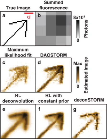
Comparison of the performance of the three deconvolution methods (RL, RL with constant prior, and deconSTORM) and two emitter localization methods (single-emitter localization with maximum likelihood fitting and multiemitter localization with DAOSTORM) for simulated fluorescence data. (a) The true locations of the simulated emitters, arranged in the shape of an arrow. (b) Sum of fluorescence data from all movie frames representing the diffraction-limited image. (c and d) Results of localization-based analysis using single-emitter maximum-likelihood fitting (c) and DAOSTORM multiemitter fitting (d). (e–g) Deconvolution-based sample estimates using the classic RL algorithm (e), RL with a constant prior (f), and deconSTORM (g). We divided the simulated movie into 16 subsets of 400 frames each and ran 2000 iterations of deconvolution for each subset. The final reconstructed image is the sum of the estimated images for each movie frame. σ is the width of the Gaussian PSF. Simulated data sets included 6400 frames, and the activation parameters, α = 0.5 and β = 0.0083, were set such that the average density of activated emitters was $\rho =1/32{\sigma }^2$ (average emitter separation d ∼ 5.7 σ, or 2.4 times the PSF full width at half-maximum).

Here, we report a computational analysis procedure that uses iterative image deconvolution, rather than single- or multiemitter localization, to estimate a superresolution image from fluorescence microscopy data sets. Our technique, deconSTORM, is based on the classic image deconvolution algorithm first proposed by Richardson and Lucy (15,16). RL deconvolution is a nonlinear iteration procedure that updates an estimate of the true image until it converges to the maximum of a statistical likelihood function (see Methods and Table 1). When applied to a conventional image in which all fluorophores are simultaneously on, deconvolution can only provide a moderate resolution enhancement because noise is amplified by the image-sharpening procedure. We reasoned that if deconvolution is applied to a sequence of many frames of fluorescence data from intermittently activated molecules, substantial resolution improvement could be achieved by taking advantage of the relative sparseness of activated fluorophores in each frame and the correlations between frames due to the intermittent activation of emitters. We compared three variants of image deconvolution: classic RL deconvolution; RL deconvolution with a prior to account for the fluorophore sparseness; and deconSTORM, a novel deconvolution procedure, to our knowledge, that takes into account both fluorophore sparseness and frame-to-frame correlation to analyze the simulated movie of the arrow (Table 1).

The classic RL deconvolution procedure resulted in a sample estimate that is sharper than the diffraction-limited fluorescence data (Fig. 2 e). However, the RL algorithm is known to converge very slowly, and in practice it is difficult to continue the iterations until convergence (19). The progressive sharpening of the sample estimate by RL deconvolution is shown in Fig. S1 in the Supporting Material (upper row). When we terminated the procedure after 2000 iterations, the sample estimate remained blurrier than the single- and multiemitter fitting results.

To optimize the deconvolution procedure for fast convergence, we first modified RL deconvolution by including in our statistical model a prior expectation of spatial sparseness in the true image (18,19). This procedure is called RL with a constant prior, since the statistical prior information was equivalent at all spatial locations and in every time frame (see Methods and Table 1). The use of statistical prior information accelerates the convergence of this deconvolution algorithm, which thus achieves a sharper image using the same number of iterations (Fig. 2 f and Fig. S1, middle row).

Finally, we developed a deconvolution procedure (deconSTORM) to further improve the resolution and convergence speed by considering the temporal correlations that result from the stochastic activation and inactivation of individual molecules. Because each molecule may remain activated during multiple frames, detection of an activated molecule in one frame increases the prior expectation of an activated molecule at the same location in subsequent and preceding frames. Similar information has been used to improve the precision of molecule localization (13). Here, we designed deconSTORM to combine the statistical model underlying RL deconvolution with a prior distribution over sample brightness that is adjusted at each pixel and time frame based on information from earlier and later frames (see Methods and Table 1). The resulting algorithm is thus an iterative, multiframe image deconvolution technique derived from a realistic statistical model of fluorescence movie data comprised of intermittently activated fluorophores. When applied to the simulated movie data, deconSTORM produced a sharper sample estimate than the other two deconvolution procedures and the single- and multiemitter localization methods (Fig. 2 g). For example, the erroneous localizations near the intersection of the three lines of the arrow in the other estimated image are largely absent in the deconSTORM image. Compared with the classic RL algorithm and RL with constant prior, deconSTORM converges in fewer iterations to a sharp, superresolution sample estimate (Fig. S1).

Quantitative comparison of the two localization methods and the three deconvolution methods

The examples described above indicate the potential of deconSTORM to analyze fluorescence microscopy data more efficiently than do existing techniques, but the performance in practice depends on parameters such as the density of activated fluorophores and the size of image features. We therefore simulated many randomly generated samples and the resulting fluorescence data with different rates of fluorophore activation, β, and thus different average densities of activated emitters/frame. For these simulations, we used samples with a uniform average emitter density; the results therefore calibrate the expected performance for specific local fluorophore density. For complex samples with spatially varying fluorophore density, the effective resolution within the image could vary with the fluorophore density. To quantify the performance of deconSTORM in comparison to the other methods, we calculated the mean-squared reconstruction error as a function of image spatial frequency (see Methods). This objective measure is analogous to the modulation transfer function used to characterize the spatial-frequency-dependent transmission of image information by an optical microscope. However, the mean-squared error captures image blurring due to both the optical instrument's PSF and the noise sources, and it is a direct measure of the practical performance of each data analysis procedure.

We found that the mean squared error, ε(k), is near zero for coarse image features corresponding to spatial frequencies below the scale set by diffraction, $k<1/\sigma$ (Fig. 3 a). When the density of simultaneously fluorescent emitters was low (e.g., $\rho =0.005/{\sigma }^2$, Fig. 3 a1), corresponding to large mean emitter separation $\left(d=14\sigma \right)$, the performance of single- and multiemitter localization procedures (black, cyan curves) matched that of deconSTORM and RL deconvolution with a constant prior (red, green). Classic RL deconvolution performed less well, because it failed to converge before the limit of 2000 iterations we had imposed (Fig. 3 b1).

Figure 3.

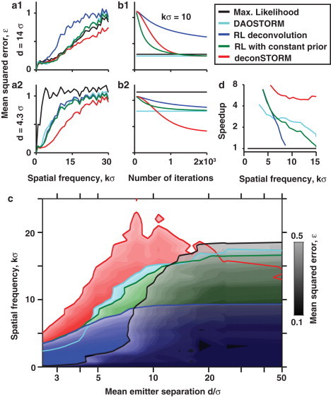
Quantitative comparison of the five analysis algorithms using simulated fluorescence movie data. (a1 and a2) Relative mean-squared error of the 2D Fourier transform of the estimated image as a function of spatial frequency, k. The activation parameter, β, was varied to produce a large average separation between simultaneously activated emitters (a1, d = 14σ) or a relatively small separation (a2, d = 4.3σ). For deconvolution results, n = 2000 iterations were used. (b1 and b2) Mean-squared error at a representative spatial frequency (k = 10/σ) as a function of the number of deconvolution iterations applied. The errors for localization-based sample estimates at this spatial frequency are shown as horizontal lines for comparison. (c) Phase diagram showing the range over which each algorithm achieves relative error, ε ≤ 0.5. (d) Expected increase in the image acquisition speed (speedup) relative to single-emitter fitting for each spatial frequency. Here, the relative acquisition speed of a superresolution image is defined as the maximum emitter density that can be used with error ε ≤ 0.5 for each method relative to that for the single-emitter localization method based on maximum-likelihood fitting. Since the time required for image acquisition is inversely proportional to the density of activated emitters/frame, the maximum density provides a measure of the gain in imaging speed.

Next, we challenged the analysis methods by simulating fluorescence data with a higher density of activated emitters $\left(\rho =0.05/{\sigma }^2\right)$, corresponding to a mean separation of only $d=4.3\sigma$ (Fig. 3, a2 and b2). For a fair comparison, we reduced the total number of movie time frames as we increased the density of activated emitters/frame, keeping the total number of frames in which each emitter was active roughly constant (see Methods). At this higher emitter density, single-emitter fitting resulted in high mean-squared error for all spatial frequencies above the conventional diffraction limit. DAOSTORM multiemitter fitting still achieved superresolution sharpening of the estimated image to some extent. Classic RL deconvolution and RL with constant prior also successfully sharpened the estimated image, achieving error profiles similar to those seen with DAOSTORM. Notably, deconSTORM substantially improved the estimated images, achieving lower error than the other analysis procedures for all spatial frequencies. For example, at k = 10/σ the mean-squared error of the deconSTORM estimate was half as large as that of the alternative deconvolution procedures and of DAOSTORM, and it was only 35% of the error of the single-emitter maximum-likelihood fitting procedure. The maximum spatial frequency that could be resolved at this density with error ε < 0.5 was k_max = 12.1/σ for deconSTORM, 6.5/σ for RL with constant prior, 6.2/σ for RL, 5.6/σ for DAOSTORM, and only 0.85/σ for single-emitter fitting.

Each method's performance as a function of spatial frequency and mean emitter separation is shown in Fig. 3 c. The red region on the left-hand side of this phase plane shows the range of image spatial frequencies that are correctly estimated by deconSTORM in moderately crowded conditions, but which are not correctly estimated by the alternative procedures. On the righthand side of the diagram, corresponding to ultrasparse conditions in which simultaneously activated fluorophores do not overlap, the single-emitter maximum-likelihood fitting procedure (black) achieves the optimal performance. In these conditions, deconvolution with a finite number of iterations does not converge to the optimal, pointlike sample estimate for each isolated emitter. DeconSTORM is thus an advantageous analysis procedure in moderately crowded conditions with mean emitter separation, d, up to ∼15σ.

Finally, we determined the potential increase in image acquisition speed that could be achieved by using deconSTORM analysis (Fig. 3 d). The data acquisition time required to reconstruct an image containing a given total density of emitters is inversely proportional to the density of activated emitters in each frame. Thus, the speedup is defined as the maximum density of activated emitters that could be imaged with low error, relative to the density required for single-emitter localization. We chose an error threshold of ε ≤ 0.5. The corresponding speedup relative to single-emitter localization is approximately fivefold or more for deconSTORM over a range of spatial frequencies up to 15/σ. Relative to multiemitter fitting with DAOSTORM, deconSTORM achieves a speedup of 2.2-fold at k = 10/σ.

Computational cost

The efficient use of all available image information by a sophisticated data analysis procedure inevitably comes at the cost of increased computational complexity. Single-emitter maximum-likelihood fitting can be performed using a fast Newton-Raphson algorithm that achieves the theoretical minimum error for localizing isolated emitters (6). Deconvolution procedures estimate an entire image, i.e., a grayscale value at each superresolution pixel, rather than a set of locations for each data frame. Because there are typically more pixels than activated emitters, deconvolution requires a greater number of computations at each iteration compared to single-emitter localization. Furthermore, convergence of the deconvolution techniques may require ∼10³ iterations, even with the use of spatial and temporal statistical information for acceleration, as in deconSTORM (Fig. 2 and Fig. S1).

We compared the time required to analyze simulated fluorescence microscopy data using a custom MATLAB routine for single-emitter fitting, as well as classic RL, RL with constant prior, and deconSTORM (Fig. S2). As expected, deconSTORM was the most computationally costly algorithm, requiring ∼10 times more computation time/frame than the other deconvolution methods and single-emitter fitting. Comparison with DAOSTORM is more difficult, because the published DAOSTORM software is based on compiled software rather than MATLAB code (12). When we compared the analysis speed of DAOSTORM with the single-emitter localization STORM analysis written in a similar program, we found that DAOSTORM required from 5- to 10-fold more computation time than did the single-emitter localization routine. We have not explored possible strategies for reducing the computational cost of deconSTORM, such as detecting and ignoring any regions of the field of view that are clearly devoid of activated emitters or analyzing multiple movie frames in parallel. The latter strategy, in particular, could lead to a significant speedup when using highly parallel computing architectures such as a cluster of graphical processing units (6,11).

Performance for experimental data from cellular imaging

To test the method's applicability to real experimental data, we used deconSTORM to analyze data from a well characterized model system for superresolution fluorescence microscopy, microtubules immunolabeled with the photoswitchable dye pair Alexa 405 and Alexa 647 (24) (see Figs. 4 and 5). Alexa 647 is photoswitchable, and pairing with Alexa 405 increases the activation rate of Alexa 647 when using a 405-nm activation laser. The fluorescence data included individual frames in which pairs (Fig. 4 a and b) or larger groups (Fig. 4, c and d) of fluorophores were simultaneously activated and produced overlapping images. Conventional STORM analysis based on single-emitter localization often identified a subset of the putative activated emitters (Fig. 4, red circles). When the emitters were sufficiently separated, DAOSTORM recovered additional localizations (Fig. 4, a and c). However, when the separation between neighboring emitters was close to σ, or when the images of three or more emitters overlapped, deconSTORM analysis extracted a greater fraction of the putative activated emitters than did either localization method (Fig. 4, c and d).

Figure 4.

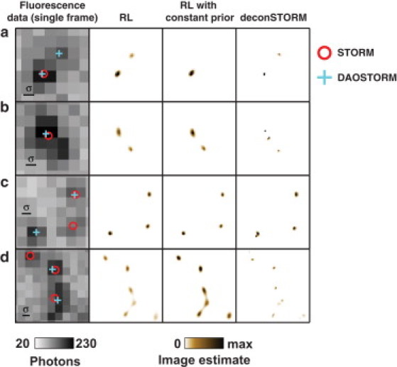
Examples of individual fluorescence data frames and corresponding sample estimates from immunohistochemically labeled microtubules. (a) STORM analysis (red circles) localizes one emitter; DAOSTORM (cyan crosses) and deconSTORM (brown pattern) identify two. RL and RL with constant prior (brown pattern) provide blurred estimates of emitter location. (b) DeconSTORM estimates a sample with three bright spots; the other methods localize one or two. (c) Three nearby peaks identified by deconvolution are not captured by either of the localization approaches alone. (d) A crowded sample containing several putative emitters. Whereas analysis by localization identifies two or three emitters, the deconvolution methods provide a more complex sample estimate.

Figure 5.

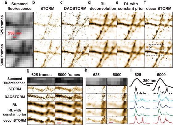
Analysis of imaging data from immunohistochemically labeled microtubules with the five methods. Images in the upper row represent data from 625 frames and those in the lower row data from 5000 frames. (a) Summed fluorescence data showing diffraction-limited resolution. (b–e) Results of analysis using single-emitter localization (23) (b) and DAOSTORM multiemitter localization (c), as well as three statistical deconvolution algorithms: RL (d), RL with constant prior (e), and deconSTORM (f). All deconvolution analyses were performed with n = 1000 iterations. (g) Magnified view of a region of interest indicated by dashed box 1 in f. (h) Magnification of dashed box 2 in f, showing a microtubule that is detected by deconSTORM but not clearly visible in the other sample estimates. (i) Cross section through each sample estimate at the location indicated by the solid box in f.

When we summed all the estimates of individual frames to obtain an estimate of the full sample (Fig. 5), deconSTORM extracted superresolution information from both isolated and overlapping images of individual fluorophores. Using only 625 frames (Fig. 5 b, upper), conventional STORM analysis based on localizing individual molecules (24) produced a grainy sample estimate with gaps in locations where no sufficiently isolated emitters could be localized. Multiemitter fitting by DAOSTORM fills in some of these gaps by detecting and localizing a greater fraction of the emitters (Fig. 5, c and i). RL deconvolution and RL with constant prior (Fig. 5, d and e) produce sample estimates which, though sharper than the conventional diffraction limit, are nevertheless not as sharp as the images estimated by localization. DeconSTORM produced a more continuous and sharper sample estimate than did the other deconvolution methods (Fig. 5 f). Even when using only 625 frames, the deconSTORM estimate was quite similar to the more refined estimate derived from 5000 frames (Fig. 5 f, lower). In addition, deconSTORM analysis detected a microtubule that is not clearly discernible in the sample estimates produced by the other analysis methods (Fig. 5 h).

Discussion

Motivated by the need to substantially improve the imaging speed of superresolution fluorescence microscopy for analyzing dynamic processes, we have developed deconSTORM, a method for analyzing data from fluorescence microscopy to estimate superresolution images of biological structures. DeconSTORM differs fundamentally from previous procedures based on single- and multiemitter localization (2–6,9–13). Rather than analyze data by estimating emitter locations and then combining the locations to form an estimated image, the deconSTORM approach directly estimates a superresolution image without explicitly localizing any emitters. Instead, an iterative deconvolution algorithm is used to maximize the statistical likelihood of a sample estimate based on the fluorescence movie data comprising multiple frames of intermittently activated fluorophores. Because existing deconvolution algorithms have not been specifically tailored to key statistical features of such data (15,16,18,19), we introduced a deconvolution algorithm that is derived from a realistic model of this imaging modality.

DeconSTORM is based on statistical principles that have been successfully applied in compressive sensing algorithms, which combine measurements from a limited number of sensors with statistical prior knowledge to reconstruct a signal with far more degrees of freedom than the measured data (20,25,26). DeconSTORM relies on statistical prior knowledge to guide image estimation, but it differs from compressive sensing in two important aspects. First, deconSTORM accounts for the Poisson distribution of fluorescence photons rather than using a Gaussian approximation, which can have suboptimal consequences (6). Second, the prior distribution of signals incorporates both the sparse structure expected of fluorescence images of the subset of activated molecules and correlations among sequences of subsequent frames expected from the stochastic dynamics of fluorophore activation and deactivation.

Although we have demonstrated deconSTORM for 2D imaging, the underlying statistical model based on linear convolution and Poisson-distributed photon statistics should also be applicable to 3D superresolution techniques based on an axial position-dependent PSF (27–29). Deconvolution-based analysis using deconSTORM should therefore be useful for 3D data sets, although the computational requirements would be increased.

Because deconSTORM analyzes the full fluorescence data set rather than a subset of well-isolated emitters, and thus allows a higher density of activated fluorophores/imaging frame, it offers a substantial increase in the image acquisition speed, critical for studying dynamic biological processes. Our validation studies using simulated and experimental data show that deconSTORM can allow an approximately fivefold or greater speedup in the collection of superresolution data for the same final image quality as single-emitter fitting techniques. We expect that image-deconvolution-based analysis will be a valuable tool for fast superresolution microscopy at high density.

References

- 1.Huang B., Babcock H., Zhuang X. Breaking the diffraction barrier: super-resolution imaging of cells. Cell. 2010;143:1047–1058. doi: 10.1016/j.cell.2010.12.002. [DOI] [PMC free article] [PubMed] [Google Scholar]
- 2.Rust M.J., Bates M., Zhuang X. Sub-diffraction-limit imaging by stochastic optical reconstruction microscopy (STORM) Nat. Methods. 2006;3:793–795. doi: 10.1038/nmeth929. [DOI] [PMC free article] [PubMed] [Google Scholar]
- 3.Betzig E., Patterson G.H., Hess H.F. Imaging intracellular fluorescent proteins at nanometer resolution. Science. 2006;313:1642–1645. doi: 10.1126/science.1127344. [DOI] [PubMed] [Google Scholar]
- 4.Hess S.T., Girirajan T.P., Mason M.D. Ultra-high resolution imaging by fluorescence photoactivation localization microscopy. Biophys. J. 2006;91:4258–4272. doi: 10.1529/biophysj.106.091116. [DOI] [PMC free article] [PubMed] [Google Scholar]
- 5.Mortensen K.I., Churchman L.S., Flyvbjerg H. Optimized localization analysis for single-molecule tracking and super-resolution microscopy. Nat. Methods. 2010;7:377–381. doi: 10.1038/nmeth.1447. [DOI] [PMC free article] [PubMed] [Google Scholar]
- 6.Smith C.S., Joseph N., Lidke K.A. Fast, single-molecule localization that achieves theoretically minimum uncertainty. Nat. Methods. 2010;7:373–375. doi: 10.1038/nmeth.1449. [DOI] [PMC free article] [PubMed] [Google Scholar]
- 7.Wolter S., Endesfelder U., Sauer M. Measuring localization performance of super-resolution algorithms on very active samples. Opt. Express. 2011;19:7020–7033. doi: 10.1364/OE.19.007020. [DOI] [PubMed] [Google Scholar]
- 8.Ram S., Ward E.S., Ober R.J. Beyond Rayleigh's criterion: a resolution measure with application to single-molecule microscopy. Proc. Natl. Acad. Sci. USA. 2006;103:4457–4462. doi: 10.1073/pnas.0508047103. [DOI] [PMC free article] [PubMed] [Google Scholar]
- 9.Burnette D.T., Sengupta P., Kachar B. Bleaching/blinking assisted localization microscopy for superresolution imaging using standard fluorescent molecules. Proc. Natl. Acad. Sci. USA. 2011;108:21081–21086. doi: 10.1073/pnas.1117430109. [DOI] [PMC free article] [PubMed] [Google Scholar]
- 10.Simonson P.D., Rothenberg E., Selvin P.R. Single-molecule-based super-resolution images in the presence of multiple fluorophores. Nano Lett. 2011;11:5090–5096. doi: 10.1021/nl203560r. [DOI] [PMC free article] [PubMed] [Google Scholar]
- 11.Huang F., Schwartz S.L., Lidke K.A. Simultaneous multiple-emitter fitting for single molecule super-resolution imaging. Biomed. Opt. Express. 2011;2:1377–1393. doi: 10.1364/BOE.2.001377. [DOI] [PMC free article] [PubMed] [Google Scholar]
- 12.Holden S.J., Uphoff S., Kapanidis A.N. DAOSTORM: an algorithm for high- density super-resolution microscopy. Nat. Methods. 2011;8:279–280. doi: 10.1038/nmeth0411-279. [DOI] [PubMed] [Google Scholar]
- 13.Cox S., Rosten E., Heintzmann R. Bayesian localization microscopy reveals nanoscale podosome dynamics. Nat. Methods. 2012;9:195–200. doi: 10.1038/nmeth.1812. [DOI] [PMC free article] [PubMed] [Google Scholar]
- 14.Dertinger T., Colyer R., Enderlein J. Fast, background-free, 3D super-resolution optical fluctuation imaging (SOFI) Proc. Natl. Acad. Sci. USA. 2009;106:22287–22292. doi: 10.1073/pnas.0907866106. [DOI] [PMC free article] [PubMed] [Google Scholar]
- 15.Lucy L. An iterative technique for the rectification of observed distributions. Astron. J. 1974;79:745–766. [Google Scholar]
- 16.Richardson W. Bayesian-based iterative method of image restoration. J. Opt. Soc. Am. 1972;62:55–59. [Google Scholar]
- 17.Shepp L., Vardi Y. Maximum likelihood reconstruction for emission tomography. IEEE Trans. Med. Imaging. 1982;1:113–122. doi: 10.1109/TMI.1982.4307558. [DOI] [PubMed] [Google Scholar]
- 18.Lingenfelter, D., J. Fessler, and Z. He. 2009. Sparsity regularization for image reconstruction with Poisson data. In Computational Imaging VII. Proceedings of the SPIE. C. A. Bouman, E. L. Miller, and I. Pollak, editors. Society of Photo Optical, San Jose, CA. 7246:72460F.
- 19.Shaked E., Michailovich O. Iterative shrinkage approach to restoration of optical imagery. IEEE Trans. Image Process. 2011;20:405–416. doi: 10.1109/TIP.2010.2070073. [DOI] [PubMed] [Google Scholar]
- 20.Chen S., Donoho D., Saunders M. Atomic decomposition by basis pursuit. SIAM J. Sci. Comput. 1998;20:33–61. [Google Scholar]
- 21.von Middendorff C., Egner A., Schönle A. Isotropic 3D nanoscopy based on single emitter switching. Opt. Express. 2008;16:20774–20788. doi: 10.1364/oe.16.020774. [DOI] [PubMed] [Google Scholar]
- 22.Small A.R. Theoretical limits on errors and acquisition rates in localizing switchable fluorophores. Biophys. J. 2009;96:L16–L18. doi: 10.1016/j.bpj.2008.11.001. [DOI] [PMC free article] [PubMed] [Google Scholar]
- 23.Thompson M.A., Lew M.D., Moerner W.E. Localizing and tracking single nanoscale emitters in three dimensions with high spatiotemporal resolution using a double-helix point spread function. Nano Lett. 2010;10:211–218. doi: 10.1021/nl903295p. [DOI] [PMC free article] [PubMed] [Google Scholar]
- 24.Bates M., Huang B., Zhuang X. Multicolor super-resolution imaging with photo-switchable fluorescent probes. Science. 2007;317:1749–1753. doi: 10.1126/science.1146598. [DOI] [PMC free article] [PubMed] [Google Scholar]
- 25.Shechtman Y., Gazit S., Segev M. Super-resolution and reconstruction of sparse images carried by incoherent light. Opt. Lett. 2010;35:1148–1150. doi: 10.1364/OL.35.001148. [DOI] [PubMed] [Google Scholar]
- 26.Coskun A.F., Sencan I., Ozcan A. Lensless wide-field fluorescent imaging on a chip using compressive decoding of sparse objects. Opt. Express. 2010;18:10510–10523. doi: 10.1364/OE.18.010510. [DOI] [PMC free article] [PubMed] [Google Scholar]
- 27.Huang B., Wang W., Zhuang X. Three-dimensional super-resolution imaging by stochastic optical reconstruction microscopy. Science. 2008;319:810–813. doi: 10.1126/science.1153529. [DOI] [PMC free article] [PubMed] [Google Scholar]
- 28.Juette M.F., Gould T.J., Bewersdorf J. Three-dimensional sub-100 nm resolution fluorescence microscopy of thick samples. Nat. Methods. 2008;5:527–529. doi: 10.1038/nmeth.1211. [DOI] [PubMed] [Google Scholar]
- 29.Pavani S.R., Thompson M.A., Moerner W.E. Three-dimensional, single-molecule fluorescence imaging beyond the diffraction limit by using a double-helix point spread function. Proc. Natl. Acad. Sci. USA. 2009;106:2995–2999. doi: 10.1073/pnas.0900245106. [DOI] [PMC free article] [PubMed] [Google Scholar]
Associated Data
This section collects any data citations, data availability statements, or supplementary materials included in this article.