Performance comparison between total variation (TV)-based compressed sensing and statistical iterative reconstruction algorithms

Abstract

Of all available reconstruction methods, statistical iterative reconstruction algorithms appear particularly promising since they enable accurate physical noise modeling. The newly developed compressive sampling/compressed sensing (CS) algorithm has shown the potential to accurately reconstruct images from highly undersampled data. The CS algorithm can be implemented in the statistical reconstruction framework as well. In this study, we compared the performance of two standard statistical reconstruction algorithms (penalized weighted least squares and q-GGMRF) to the CS algorithm. In assessing the image quality using these iterative reconstructions, it is critical to utilize realistic background anatomy as the reconstruction results are object dependent. A cadaver head was scanned on a Varian Trilogy system at different dose levels. Several figures of merit including the relative root mean square error and a quality factor which accounts for the noise performance and the spatial resolution were introduced to objectively evaluate reconstruction performance. A comparison is presented between the three algorithms for a constant undersampling factor comparing different algorithms at several dose levels. To facilitate this comparison, the original CS method was formulated in the framework of the statistical image reconstruction algorithms. Important conclusions of the measurements from our studies are that (1) for realistic neuro-anatomy, over 100 projections are required to avoid streak artifacts in the reconstructed images even with CS reconstruction, (2) regardless of the algorithm employed, it is beneficial to distribute the total dose to more views as long as each view remains quantum noise limited and (3) the total variation-based CS method is not appropriate for very low dose levels because while it can mitigate streaking artifacts, the images exhibit patchy behavior, which is potentially harmful for medical diagnosis.

1. Introduction

The concept of using iterative methods to reconstruct x-ray computed tomographic (CT) images has been around for several decades. In fact, it was used in the early development of EMI CT scanners (Hounsfield 1968). Limited by the available computational power, iterative image reconstruction methods were replaced by the much more computationally efficient analytical image reconstruction methods. The defacto standard for reconstruction on the state-of-the-art commercial CT scanners is the filtered backprojection (FBP) algorithm. However, given the increase in computational power which may be leveraged to solve the reconstruction problem, iterative CT reconstruction is moving closer to clinical practice. As a result of the dose benefits of statistical image reconstruction (SIR) algorithms and the constant computational improvements, SIR algorithms will most likely have a predominate place in future CT technology.

There are two general categories of iterative image reconstruction algorithms. One approach is algebraic and is based upon solving a system of linear equations, which is often referred to as an algebraic reconstruction technique (ART) (Gordon et al 1970, Gordon and Herman 1974, Herman 1980) or its variants with different update strategies (Gilbert 1972, Andersen and Kak 1984, Kawata and Nalcioglu 1985, Wang et al 1996, Jiang and Wang 2003a, 2003b). The other approach utilizes the knowledge of the underlying physics, namely the understanding of the statistical distribution resulting from the x-ray interaction process. There is inherent uncertainty in each projection measurement due to the photon statistics. Thus, the aim of the image reconstruction process is to estimate the best image, i.e. the image which has the highest probability to match the measured projection data. Additionally, some given prior information about the image object is frequently assumed such that the reconstructed image does not contain unphysical fluctuations. This category of image estimation methods is generally referred to as SIR (Rockmore and Macovski 1976, 1977, Shepp and Vardi 1982, Lange and Carson 1984, Geman and McClure 1985, Green 1990, Geman et al 1992, Bouman and Sauer 1993, Sauer and Bouman 1993, Fessler and Hero 1994, Hudson and Larkin 1994, Lange and Fessler 1995, Erdogan and Fessler 1999, Sukovic and Clinthorne 2000, Beekman and Kamphuis 2001, De Man et al 2001, Elbakri and Fessler 2002, Kachelriess et al 2003, Li et al 2005, Thibault et al 2007, Zbijewski et al 2007, Wang et al 2008, Wang et al 2009).

In general, there are several attractive features of iterative image reconstruction methods: first, artifacts due to imperfect data are localized in the reconstructed images. An example where this feature improves image reconstruction is the case of metal artifacts (Wang et al 1995, Wang et al 1996, Hsieh 1998, De Man et al 1999, De Man et al 2000). The second feature is that iterative methods are more forgiving for data truncation at a given view angle and/or view truncation as in limited view angle problems (e.g. tomosynthesis imaging) (Persson et al 2001, Li et al 2002, Kolehmainen et al 2003, Yu and Wang 2009). Third, there are no inherent assumptions about the projection acquisition geometry and the same algorithm may be used directly for multiple geometries. Fourth, view aliasing artifacts due to view angle undersampling are also mitigated by iterative image reconstruction algorithms. Fifth, when a statistical iterative image reconstruction algorithm is used, one can effectively incorporate the knowledge of photon statistics into the image reconstruction process to reduce the noise variance in the final reconstructed images (Sukovic and Clinthorne 2000, De Man et al 2001, Elbakri and Fessler 2002, Li et al 2005, Thibault et al 2007, Wang et al 2008, 2009). Additionally, it is possible to incorporate the knowledge of the x-ray spectra into the forward model to more accurately account for physical effects such as beam hardening (De Man et al 2001). The ability to properly account for photon statistics is particularly important in modern CT technology since there is increasing concern over the delivered radiation dose to patients (Brenner and Hall 2007). This issue is attracting attention from the general public, healthcare providers, the medical physics community and CT manufacturers.

When an iterative image reconstruction algorithm is formulated, several scientific issues must be addressed. The first issue is the convergence and the speed of the convergence of the algorithm. The second issue is the optimization method to solve the minimization or maximization problem. Historically, iterative reconstruction has been implemented in nuclear medicine for clinical procedures before it has been used for CT reconstruction (Shepp and Vardi 1982). The acquired projection data and image reconstruction matrices in nuclear imaging are much smaller than CT imaging. This is due to the relatively simple imaging task of reconstructing the distribution of a radioactive tracer. Additionally, the intrinsic spatial resolution of these systems is limited by the interaction processes. Therefore, the computational load for these reconstructions is significantly lower than for general diagnostic CT, where the data sets are much larger and the objects to be reconstructed contain more fine detailed structures. Since the aim of CT reconstruction is to generate images which have more spatial frequency content than typical nuclear medicine images, it is fundamentally important to understand the conditions for accurate image reconstruction of an image object with the rich spatial frequency content. Since most of the iterative reconstruction algorithms were initially formulated and evaluated for nuclear medicine data, these issues have not been thoroughly studied for CT data.

The image reconstruction community experienced a dramatic revitalization when Candes et al published their seminal works (Candes et al 2006, Donoho 2006) on compressed sensing (CS). If we put CS in the context of the body of iterative image reconstruction algorithms, one may view it just as another algorithm (Geman et al 1990, Geman and Reynolds 1992, Geman and Yang 1995, Panin et al 1999, Persson et al 2001, Combettes and Pesquet 2004). However, what makes the CS theory so important is that it addressed the sampling condition for accurate reconstruction of an image object. It has been mathematically proven that one only needs ∼SlnN samples to accurately reconstruct a sparse image with S significant image pixels in an N × N image. This sampling condition is significantly different from the conventional Shannon/Nyquist sampling condition where the number of required samples is determined by the highest frequency component of the image object. As a result, what CS theory offers in practice is that an image object may be accurately reconstructed using very few samples.

Using simple high-contrast digital phantoms such as the high-contrast Shepp–Logan phantom, it has been demonstrated that objects can be accurately reconstructed with only ∼20 view angles (Candes et al 2006, Sidky et al 2006, Sidky and Pan 2008). However, in clinical practice, the image object is far more complicated than the high-contrast Shepp– Logan phantom and soft tissue contrast is often important for diagnosis. Therefore, it is very important to have an estimate for the number of projections needed to reconstruct an acceptable clinical image. Since the number of view angles in the CS theory is image object dependent, it is crucial to answer this question using projection data containing realistic anatomical background structures (Herman and Davidi 2008). In addition to this, since it is natural to view the CS algorithm as just another iterative image reconstruction algorithm, it is also interesting to investigate how the other well-known iterative image reconstruction algorithms perform under the same undersampling conditions and the same noise conditions. These questions motivated the work presented in this paper. Namely, using a human cadaver head as our image object, we study the performance of the CS algorithm and other well-known SIR algorithms in x-ray CT. Several figures of merit including the relative root mean square error and a quality factor which accounts for the noise performance and the spatial resolution were introduced to objectively evaluate reconstruction performance. A comparison was made between the three algorithms for a constant undersampling factor comparing different algorithms at several dose levels. To facilitate this comparison, the original CS method was also formulated in the framework of the SIR algorithms.

2. Methods and materials

2.1. Brief review of statistical image reconstruction (SIR) algorithms

2.1.1. Model of x-ray computed tomography (CT) data acquisition system

For simplicity, we will use a monochromatic x-ray spectrum to illustrate our data acquisition model. The x-ray photons emanate from the x-ray tube and are attenuated by the image object according to Beer's law:

$$I=I_0\text{exp}\left(-{\int }_l\mu \left(x,y,z\right)\text{d}l\right),$$ (1)

where I is the detected photon number, I₀ is the entrance photon number at a given detector pixel and l denotes the straight line from the x-ray focal spot to the detector pixel, it is also referred to as the x-ray path. The line integral is performed along the x-ray path.

From equation (1), a logarithmic operation is performed to obtain the so-called projection data, which is the line integral in equation (1):

$$y=\text{ln}\frac{I_0}{I}={\int }_l\mu \left(x,y,z\right)\text{d}l$$ (2)

The image reconstruction process is then to estimate the attenuation coefficients, μ, from a series of line integral values (i.e. the projection data). In image reconstruction, the attenuation coefficients may be digitized into the so-called pixel/voxel representation:

$$\mu \left(x,y,z\right)=\sum _{i\in S}{\mu }_i{w}_i\left(x,y,z\right)$$ (3)

In this notation, S denotes the index of the set of N voxel locations, i is the voxel index and w_i(x, y, z) is the basis function which has the following shift-invariant property:

$$w_{(i_1,i_2,i_3)}\left(x,y,z\right)=w_{\left(0,0,0\right)}(x-i_1\Delta x,y-i_2\Delta y,z-i_3\Delta z)$$ (4)

where Δx, Δy and Δz are spatial sampling periods of the image representation along the x-, y- and z-axes and i = (i₁, i₂, i₃) is the indices of the voxel location in a three-dimensional grid. Substituting representation equation (3) into line integral equation (2), one obtains:

$$y=\sum _{i\in S}{\mu }_i{\int }_l{w}_i\left(x,y,z\right)\text{d}l=\sum _{i\in S}{A}_{\mathit{\text{ji}}}{\mu }_i=A\mu$$ (5)

where the system matrix A is given by

$$A_{\mathit{\text{ji}}}={\int }_{l_j}{w}_i\left(x,y,z\right)\text{d}l.$$ (6)

Namely, the system matrix is the line integral of the basis function w_i(x, y, z) along the jth x-ray path which is determined by the focal spot position and the detector pixel position. Obviously, the system matrix is independent of the image object. Rather, it is only dependent on the basis function and the source and detector positions.

Equation (5) gives a system of linear equations with variables μ_i, which is the local distribution of attenuation coefficients at the voxel i = (i₁, i₂, i₃). Based on this equation, different algebraic methods have been developed to iteratively solve the linear system to obtain the attenuation coefficients. This category of iterative methods is generally referred to as ART in this paper (Herman 1980).

2.1.2. Statistical models

In equation (5), the entire process of data acquisition is modeled as a deterministic process. There is no explicit model to account for the intrinsic photon statistics which introduce noise into the measurements. Although it has not been expressed explicitly, the quantities above which we assume deterministic measurements are average values over each detector pixel and x-ray exposure time window. To better model the x-ray interaction and detection process, a statistical model has been developed in the literature and is briefly reviewed here.

A feasible model for photon counts, I_j, at the detector element j is to assume that each reading of counts, I_j, is independent of the other readings of counts in neighboring pixels and that I_j follows a Poisson distribution with the expectation value Ī_j. Under this assumption, the joint probability distribution of this counting process, given a distribution of the attenuation coefficients, P(I∣μ), is given by

$$P\left(I|\mu \right)=\prod _{j=1}{p}_{\text{poisson}}(I_j,{\overline{I}}_j)=\prod _{j=1}\frac{{({\overline{I}}_j)}^{I_j}}{I_j!}\text{exp}(-{\overline{I}}_j)$$ (7)

where the expectation value Ī_j is given by

$${\overline{I}}_j={\overline{I}}_{j0}\text{exp}(-y_j)={\overline{I}}_{j0}\text{exp}(-{\left[A\mu \right]}_j).$$ (8)

Using equation (7), the log-likelihood function, L(I∣μ) = ln P(I∣μ), is given by

$$L\left(I|\mu \right)=-\sum _j\{{\overline{I}}_{j0}\text{exp}(-{\left[A\mu \right]}_j)+I_j({\left[A\mu \right]}_j-\text{ln}{\overline{I}}_{j0})-\text{ln}{I}_j!\}.$$ (9)

Using the log-likelihood function, the image reconstruction problem is formulated as the problem of maximizing the log likelihood given by equation (9). By ignoring the irrelevant terms in equation (9) in the optimization process, the image reconstruction problem is formulated as

$$\widehat{\mu }=\text{arg}\underset{\mu }{\text{min}}\sum _j\{{\overline{I}}_{j0}\text{exp}(-{\left[A\mu \right]}_j)+I_j{\left[A\mu \right]}_j\}.$$ (10)

However, it is difficult to directly minimize the above objective function. The most popular method to minimize this objective function is the expectation-minimization (EM) method (Rockmore and Macovski 1976, Dempster et al 1977, Rockmore and Macovski 1977, Shepp and Vardi 1982, Lange and Carson 1984, Fessler and Hero 1994, Hudson and Larkin 1994). The ordered subsets principle was also used to accelerate the convergence of the algorithm (Erdogan and Fessler 1999, Beekman and Kamphuis 2001, Kachelriess et al 2003, Zbijewski et al 2007). To reduce the noise in the reconstructed images, the image reconstruction process is also reformulated using the well-known Bayesian rule:

$$P(I|\mu )P(\mu )=P(\mu |I)P(I).$$

Instead of maximizing the probability P(I∣μ), the image reconstruction task is to maximize a posteriori (MAP) (Green 1990, Lange and Fessler 1995) function P(μ∣I):

$$P\left(\mu |I\right)=\frac{P\left(I|\mu \right)P\left(\mu \right)}{P\left(I\right)}.$$ (11)

The maximization is carried out by maximizing the logarithmic of the a posteriori P(μ∣I), L_p(I∣μ) = ln P(μ∣I). As a result, instead of minimizing the objective function given in equation (10), the following modified objective function is minimized:

$$\widehat{\mu }=\text{arg}\underset{\mu }{\text{min}}\left\{\sum _j{\overline{I}}_{j0}\text{exp}(-{\left[A\mu \right]}_j)+I_j{\left[A\mu \right]}_j-\text{ln}P\left(\mu \right)\right\}.$$ (12)

The meaning of the term ln P(μ) in equation (12) is the prior knowledge about the image object. This term is also often called the regularization term, U(μ), in the literature. Thus, the general form of SIR is to minimize the following objective function:

$$\widehat{\mu }=\text{arg}\underset{\mu }{\text{min}}\left\{\sum _j{\overline{I}}_{j0}\text{exp}(-{\left[A\mu \right]}_j)+I_j{\left[A\mu \right]}_j+U\left(\mu \right)\right\}.$$ (13)

In x-ray CT imaging, even when the product of the tube current and the exposure time (mAs) is relatively low, the number of detected photons per detector channel per projection is still typically over 1000 photons. In this case, the value of the probability density in equation (7) can be well approximated by a Gaussian distribution. As a result, equation (13) can be expressed in the following manner:

$$\widehat{\mu }=\text{arg}\underset{\mu }{\text{min}}\left\{\frac{1}{2}{\left(y-A\mu \right)}^{T}D\left(y-A\mu \right)+U\left(\mu \right)\right\}$$ (14)

where D is the diagonal matrix with coefficients d_j that represent the maximum likelihood estimates of the inverse of the variance of the projection measurements: d_j = Ī_j. Actually, equation (14) can be readily derived using Taylor expansion of function Ī_j0 e^−x + I_jx around the mean value, x̄_j = y_j of the variable x_j = [Aμ]_j, where the irrelevant constant terms in the expansion have been dropped leaving the expression given in equation (14).

In this paper, the objective function (14) will be used to discuss the performance of the SIR algorithms with different choices of the prior model U(μ).

2.1.3. Regularization terms

Smoothness prior and the penalized weighted least square (PWLS) algorithm

The penalized weighted least square (PWLS) approach for iterative reconstruction of x-ray CT images has been studied by Herman (1980) and Sauer and Bouman (1993). Fessler (Fessler and Hero 1994) extended the iterative PWLS method to positron emission tomography (PET). Sukovic and Clinthorne (2000) applied it to dual energy CT reconstruction. It is now a widely used statistical reconstruction algorithm (Wang et al 2009). This algorithm uses the prior knowledge that the intensity of adjacent pixels in the image should vary smoothly. The expression for the regularization term for the quadratic PWLS method is given by

$$U\left(\mu \right)=\beta \sum _{\left\{j,k\right\}\in C}{b}_{j,k}{({\mu }_j-{\mu }_k)}^2$$ (15)

where β is a scalar determined empirically to control the prior strength relative to the noise model over the local neighborhood defined by the set C of all pairs of neighboring pixels (8 pairs in the 2D case and 26 pairs in the 3D case), and b_{j, k} are the directional weighting coefficients.

q-generalized Gaussian Markov field (q-GGMRF) prior

Recently, Thibalt et al proposed to use a q-generalized Gaussian Markov random field (q-GGMRF) prior as U(x), in which the regularization term is given by (Dempster et al 1977):

$$U\left(\mu \right)=\beta \sum _{\left\{j,k\right\}\in C}{b}_{j,k}\frac{{|{\mu }_j-{\mu }_k|}^p}{1+{\left|\frac{{\mu }_j-{\mu }_k}{c}\right|}^{p-q}}.$$ (16)

One of the important features of this regularization term is that it includes many existing statistical algorithms as special cases when different values are selected for the parameters, p and q. The second important feature of the q-GGMRF prior is that the objective function equation (14) together with equation (16) is convex provided that the parameters satisfy the following condition: 1 ≤ q ≤ p ≤ 2. This makes the minimization tractable in practice. The familiar regularization functions used in the literature are listed below with specific parameter values:

1. p = q = 1, equation (16) reduces to the Geman prior (Geman and Reynolds 1992, Geman et al 1992). This is the prior closely related to the total variation norm which will be discussed in next subsection.

2. p = q = 2: Gaussian prior, which corresponds to the quadratic PWLS algorithm discussed above (Herman 1980, Sauer and Bouman 1993, Fessler and Hero 1994, Sukovic and Clinthorne 2000, Wang et al 2009). For simplicity, we refer it to as PWLS in this paper.

3. p = 2; q = 1: approximate Huber prior (Geman and McClure 1985)

4. 1 < q = p ≤ 2: generalized Gaussian MRF (Bouman and Sauer 1993)

5. 1 ≤ q < p ≤ 2: q-generalized Gaussian MRF (Thibault et al 2007).

2.2. Brief review of the compressive sampling/compressed sensing (CS) method

According to standard image reconstruction theory (Kak and Slaney 2001) in CT, in order to reconstruct an image without aliasing artifacts, the view angle sampling rate must satisfy the Shannon/Nyquist sampling theorem. This assumes no a priori knowledge of the object. However, when some prior information about the image is available and appropriately incorporated into the image reconstruction procedure, an image can be accurately reconstructed even if the Shannon/Nyquist sampling requirement is violated. For example, if one knows that a target object is circularly symmetric and spatially uniform, only one view of parallel-beam projections is needed to accurately reconstruct the linear attenuation coefficient of the object. Another extreme example is that if one knows that a target image consists of only two isolated pixels, then two orthogonal projections are sufficient to accurately reconstruct the image. Along the same logic line, one can easily convince oneself that the Shannon/Nyquist sampling requirement may be significantly violated if we know that a target image only consists of a small number of sparsely distributed pixels. However, when more and more isolated non-zero image pixels are present, it is highly nontrivial to generalize these special cases into a rigorously formulated image reconstruction theory. Fortunately, this has been recently accomplished by mathematicians in a new image reconstruction theory: CS (Candes et al 2006, Donoho 2006). It has been rigorously proven that an N × N image can be accurately reconstructed from ∼S ln N Fourier samples using a nonlinear optimization process provided that there are only S significant pixels in the image and the Fourier samples are randomly acquired. The randomness requirement is not mandatory in practice. The requirement was imposed in the mathematical proof to avoid some very special cases in signal restoration, for example, the well-known ‘Dirac Comb’ signal train. In this case, the mathematical proof may fail if the sampling pattern is not random. However, in the experimental and clinical data acquisitions, these types of extremely idealized signals are not typically encountered.

Although the mathematical framework of CS is elegant and promising, its relevance in CT imaging relies on whether CT images are sparse. If an image is not sufficiently sparse, the CS algorithms will not be directly applicable to the problem. Fortunately, in CS theory, one can apply a sparsifying transform (ψ), to increase image sparsity. In the literature (Candes et al 2006, Donoho 2006), the discrete gradient transform and wavelet transforms are frequently used for this purpose. The basic idea is to reconstruct the sparsified image first, then apply a de-sparsifying (ψ⁻¹) transform to obtain the target image. In practice, the de-sparsifying transform does not have to be explicitly available. An iterative procedure is used to perform the de-sparsifying transform during the image reconstruction process. In other words, the image reconstruction process in CS invokes a sparsifying transform explicitly and its inverse is part of the iterative reconstruction algorithm. Mathematically, the CS method reconstructs an image by solving the following constrained minimization problem:

$$\underset{\mathbf{\text{x}}}{min}{\left|\Psi \mathbf{\text{x}}\right|}_1,s.t.A\mathbf{\text{x}}=\mathbf{\text{y}}.$$ (17)

where ψ is a sparsifying transform. The l₁ norm of an N-dimensional vector x⃗ is defined as ${\left|\overrightarrow{x}\right|}_1={\sum }_{i=1}^N|x_i|$. This constrained minimization problem can be solved using a classical method such as projection onto a convex set (POCS) in which the data consistency condition, i.e. Aμ = y, is applied algebraically. In this implementation, the data enforcement step and the minimization step are implemented in an alternating manner (Sidky et al 2006, Chen et al 2008a, 2008b, Leng et al 2008, Sidky and Pan 2008, Chen et al 2009). When the problem in equation (17) is solved in this manner, the data enforcement step corresponds to the ART method presented in section 2.1. The potential drawback of this implementation in medical imaging is that the noise is not modeled.

2.3. Compressed sensing algorithm in the framework of statistical image reconstruction

The primary purpose of this paper is to investigate the performance of the CS method and other well-known SIR methods. To facilitate this comparison, we reformulate the CS method in equation (17) into the SIR framework. This can be done by incorporating the quadratic noise model given in equation (14) into the CS framework in the following manner:

$$\widehat{\mu }=\text{arg}\underset{\mu }{\text{min}}\left\{\frac{1}{2}{\left(y-A\mu \right)}^{T}D\left(Y-A\mu \right)+\beta {\left|\Psi \mu \right|}_1\right\}.$$ (18)

The objective function in equation (18) is convex since the summation of two convex functions preserves convexity.

Although there are many different choices for the sparsifying transform and the choice may be application dependent, a commonly used sparsifying transform is the total variation (TV) of the image object which is given by

$$TV(\mu )=\sum _{m.n,k}\sqrt{{({\mu }_{m+1,n,k}-{\mu }_{m,n,k})}^2+{({\mu }_{m,n+1,k}-{\mu }_{m,n,k})}^2+{({\mu }_{m,n,k+1}-{\mu }_{m,n,k})}^2.}$$ (19)

The total variation norm was first introduced by Osher et al (Rudin et al 1992) in edge-preserving image denoising processes. Over the past decade or so, the TV-norm was also investigated in nuclear medicine and limited view angle tomosynthesis studies (Persson et al 2001, Li et al 2002, Kolehmainen et al 2003, Velikina et al 2007).

2.4. Algorithms used for the performance comparison in this paper

In this study, we will investigate the performance of the statistical CS method defined by equations (18) and (19) and two other popular SIR algorithms in CT image reconstruction: the PWLS method and q-GGMRF methods. As we emphasized above, the PWLS method can also be viewed as a special case of the general q-GGMRF method. However, since the PWLS is perhaps the most popular and is a simple SIR algorithm, we still listed it as a separate algorithm in this paper. Within the large parameter space of the q-GGMRF method, the following parameter selection was used in this work:

$$p=2,q=1.2,c=10.$$ (20)

This choice is based on the detailed study presented by Thibault et al (2007). They concluded that at this specific choice of parameters, a good compromise can be achieved between spatial resolution, low-contrast sensitivity and high-contrast edge preservation at a fixed noise level.

2.5. Minimization technique

There are many different schemes to minimize the objective function (De Man et al 2005). In this paper, to ensure that there is an unbiased comparison, the same minimization scheme will be used, the Gauss–Siedel method (Sauer and Bouman 1993, Bouman and Sauer 1996). In this method, the optimization is performed in a voxel-by-voxel manner and the minimization process is reduced to a one-dimensional search since all other image elements are fixed during the update of a given voxel. The voxels are updated in a random but fixed order to minimize the correlation between adjacent updates and maximize convergence speed. Each one-dimensional optimization computes an estimate for μ_j at iteration (n + 1) from μ at iteration (n) based on the following update:

$${\widehat{\mu }}_j^{\left(n+1\right)}=\text{arg}\text{min}\left\{\sum _i\frac{d_i}{2}{\left(y_i-\sum _k{A}_{\mathit{\text{ik}}}{\mu }_k^{\left(n\right)}+A_{\mathit{\text{ij}}}({\mu }_j^{\left(n\right)}-{\mu }_j)\right)}^2+U\left(\mu \right)\right\},$$ (21)

where ${\mu }_j^{n+1}$ can be obtained by computing the root of

$$\frac{\partial }{\partial {\mu }_j}\left[\sum _i\frac{d_i}{2}{\left(y_i-\sum _k{A}_{\mathit{\text{ik}}}{\mu }_k^{\left(n\right)}+A_{\mathit{\text{ij}}}({\mu }_j^{\left(n\right)}-{\mu }_j)\right)}^2+U\left(\mu \right)\right]=0.$$ (22)

In our implementation, a simple half-interval search is performed to search for the root.

2.6. Experimental data acquisitions

In this paper, a human cadaver head was used as our image object. Realistic human anatomy was selected to answer the question of how many view angles of projection data are needed for an acceptable image reconstruction in medical CT exams. The cadaver head was scanned using the Varian Trilogy on board imager cone beam CT system (Varian Medical System, Palo Alto, California, USA). Four scans were performed at four different dose levels: 80 mA-10 ms, 40 mA-10 ms, 20 mA-10 ms, ans 10 mA-5 ms. The detector used is 397.3 mm × 298 mm and is separated into 1024 × 768 pixels. To reduce the computation load, a 2 × 2 binning was used so that the detector matrix is 512 × 384. In total, 640 projections were acquired over a 60 s rotation through 360°. A uniformly spaced view angle data decimation scheme was used to obtain undersampled data sets using the acquired 640 view angles.

2.7. Image evaluation methods

2.7.1. Reconstruction accuracy

In this paper, in order to evaluate the reconstruction accuracy of each iterative image reconstruction algorithm, the filtered backprojection (FBP) image reconstruction algorithm was used to reconstruct the reference image from 640 view angles. The relative image reconstruction error was then calculated for the images reconstructed from each iterative reconstruction algorithm under different conditions. The following definition is used for the relative root mean square error (RRME), which characterizes the reconstruction accuracy:

$$\text{RRME}=\sqrt{\frac{{\sum }_{i,j}{(I_{i,j}^{\text{iter}}-I_{i,j}^{\text{ref}})}^2}{{\sum }_{i,j}{(I_{i,j}^{\text{ref}})}^2}.}$$ (23)

The comparison of RRME is plotted for each algorithm under different angular sampling conditions and for different algorithms under the same angular sampling and radiation dose conditions.

2.7.2. Quantification of streaking artifacts

In order to quantify the undersampling streaking artifacts, a metric based on the TV values of an image slice was introduced (Leng et al 2008). We will extend this metric to equation (24) to quantify the resulting undersampling streaking artifacts in this paper. A larger TV value corresponds to stronger streaking artifacts. Due to the inevitable variation of human anatomy which will also contribute to the TV values, the streaking level is quantified by the following streaks indicator (SI):

$$\text{SI}=\text{TV}(I-I_{\text{ref}}).$$ (24)

In this metric, contributions of the anatomical variation in the TV values of the image are subtracted to emphasize the contributions from streaking artifacts in the reconstructed images. Please note that the mismatch of spatial resolutions in I and I_eff will also cause an increase in the SI value. Therefore, when the metric SI is interpreted in results, one should focus on the relative change of SI values from one sampling scheme to another, not the absolute SI values.

2.7.3. Estimation of spatial modulation transfer function (MTF) and noise variance

In CT quality assurance practice, both spatial resolution and noise variance levels are key parameters to characterize the performance of a CT imaging system (Hsieh 2003, Kalender 2005). The spatial resolution is often measured using a wire phantom and the noise variance is often measured using a uniform water phantom. However, when a nonlinear image reconstruction algorithm such as the statistical CS algorithm is used, these simple phantoms are not appropriate since the final image performance may be dependent on the image object. In this paper, we will estimate these parameters within the reconstructed images. Fine nasal structures were used for the estimation of the spatial resolution (figure 1(a)). In order to minimize the influence of the spatial correlation on our measured noise parameter, we have utilized a distributed ROI. Rather than averaging the pixels over a local ROI, pixels throughout the image were selected that had attenuation values in the fully sampled FBP within a narrow range (figure 1(b)). The standard deviation within the reconstruction values was calculated using these pixels as the ensemble.

Figure 1.

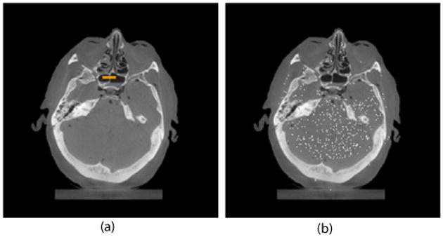
The image slice used in the evaluation of multiple algorithms (FBP fully sampled) displayed with window and level parameters of 0 0.05 mm⁻¹, (a) demonstration of the thin bone used for the in vivo MTF and (b) demonstration of the image pixels with approximately the same value 0.021045 ± 0.000045 mm⁻¹ used in the distributed ROI.

The line profile through a small nasal bone was used to measure the spatial resolution. The results from fully sampled FBP reconstructions are used as the ‘ground truth’, while the results from undersampled iterative reconstructions are used as ‘measurements’. A Gaussian fit was used to get a smooth profile. A deconvolution step was then used to extract the line-spread function and the relative MTF was calculated by taking the magnitude of the Fourier transform. Although the MTF may be over-estimated with this technique, we are only concerned with the relative performance of different algorithms in this study and thus do not require an absolute measurement of the MTF.

2.7.4. Image quality Q-factor

When one compares the noise performance of two CT image systems or two image reconstruction algorithms, the spatial resolution should be matched. Otherwise, the noise measurement becomes meaningless since one can always reduce the noise variance by sacrificing the spatial resolution. However, matching the spatial resolution exactly is challenging in practice. In order to avoid the need for a direct match of spatial resolution in system evaluation, a quality factor was introduced (Kalender 2005) which combines the influence of both noise variance and spatial resolution in a single quality factor Q. Higher Q-factors signify superior performance. In this paper, the Q-factor is used to evaluate the performance of statistical CT image reconstruction algorithms under different sampling conditions and different radiation dose levels. The definition of Q is given by

$$Q=c\frac{1}{{\sigma }^2\cdot {\rho }^{-3}\cdot S\cdot D},$$ (25)

where c is a constant, ρ is the characteristic spatial frequency chosen by selecting a point on the MTF curve such at 10% or 50% or the maximum value, S is the slice thickness, D is the radiation dose and σ² is the noise variance.

2.8. Selection of control parameter β

The parameter β is used to control the prior strength relative to the noise model over the local neighborhood. In our image reconstruction procedure, a series of β parameters were tested for each experimental case. After images were reconstructed, the noise variance, spatial resolution and streak index (SI) were estimated from the reconstructed images. The value of β used in the comparative reconstructions was selected based upon these measurements. In the first step, an empirical threshold was set for the streak index such that values of β that generated images with a large amount of streaks would be eliminated. For each algorithm, the average SI over all β values was calculated, and all β values which generated images with a higher than average SI were eliminated. Using the estimated noise variance and spatial resolution, the Q-factor was also calculated as a function of β. From the remaining β values, the β value which generates images with the highest Q value was selected for the comparative studies, as demonstrated in figure 2. In addition, resolution-noise tradeoff curves were generated using the estimated noise variance and spatial resolution. In our experimental studies, we found that this selection corresponded to a good compromise of the reconstruction parameters and yielded a visually ‘optimal’ image. In a specific application, one may want to sacrifice spatial resolution for a better noise performance or vice versa. In this case, the resolution-noise tradeoff curve can be used for guidance in selection of the β parameter.

Figure 2.

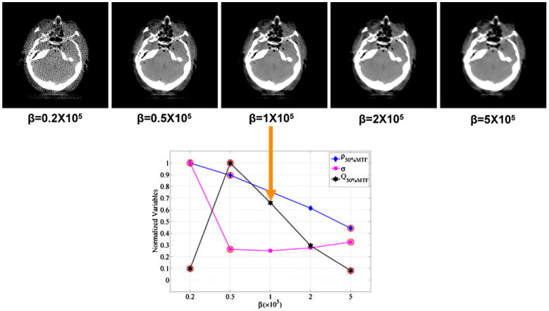
Demonstration of the selection procedure for the β parameter in the comparative studies. The points which have been circled have above average SI values and are eliminated from the selection process. From the remaining points, the image with the highest Q value is selected to determine the choice of β. This example is for qGGMRF with 160 views at 0.8 mAs.

3. Results

In this section, experimental results and evaluations are presented. First, we will present results of a performance study comparing the algorithms at several view sampling rates. Second, we will present results of a study comparing each algorithm at different dose rates (mAs/view). Third, results will be presented for a comparison of each algorithm under the condition of fixed total amount of radiation dose while varying the view sampling. Finally, we present the control parameter β used in our image reconstructions.

3.1. Algorithm performance comparison with varying view angle sampling

In the first study, we fixed the dose per view at 0.8 mAs/view (80 mA-10 ms). The images were reconstructed using PWLS, q-GGMRF and CS algorithms where the total number of view angles was 320, 160, 107, and 80. The reconstructed images are presented in figure 3. In the PWLS and q-GGMRF reconstructions, we can reconstruct streak-free images with 320 views; however, in the case of further undersampling of the data to 160 views, streaking artifacts become apparent. In contrast, in the CS reconstructions, the resulting image with 320 views yields streak-free results from visual inspection. Additionally with 160 views, there are not many obvious streaking artifacts. When 107 views were used, streaks are present in all of the reconstructed images. All comparative images throughout the paper are displayed using the same window and level parameters of 0.015 0.026 mm⁻¹.

Figure 3.

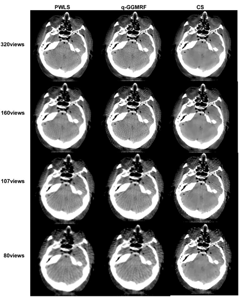
Qualitative comparison of reconstructed images using the PWLS, q-GGMRF and TV-based CS algorithms at four different view angle sampling rates: 320, 160, 107 and 80.

The above results demonstrated that the required number of view angles for an acceptable streak-free reconstruction lies between 160 and 320. Thus, approximately more than 200 view angles are required for the both PWLS and q-GGMRF algorithm to reconstruct streak-free images. In contrast, the required number of view angles can be lowered to between 100 and 160 view angles for total variation-based CS algorithm while still achieving relatively streak-free reconstruction.

Using the streak indication (SI) quantity as the figure of merit, the level of streaking artifacts was calculated for each of the reconstructions, these results are presented in figure 4. From the plot in figure 4 and visual observation of figure 3, one may conclude that streaking artifacts are insignificant when the SI values are lower than 45. Using 45 as the threshold value, one can conclude that, approximately, 200 or more view angles are needed for both the PWLS and q-GGMRF algorithms to achieve streak-free reconstruction while more than 100 views are needed for TV-based CS algorithm to achieve relatively streak-free reconstruction.

Figure 4.

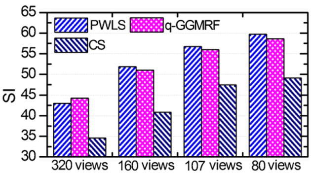
Plot of the streaking artifact indication (SI) versus different numbers of view angles and different algorithms.

3.2. Comparison of different algorithms at different dose levels with 320 views

From the performance study varying the view angle sampling, we can achieve relatively streak-free reconstruction for all of the algorithms when the number of view angles is 320. In this section, we fix the total number of view angles at 320 and compare the performance of the algorithms at different noise levels, which is controlled by the mAs/view.

The results for four different dose levels of 0.8, 0.4, 0.2 and 0.05 mAs/view are given in figure 5. For the PWLS and q-GGMRF algorithms, when the dose level is decreased, more noise appears in the images, which is anticipated from imaging physics. In contrast, in the TV-based CS reconstructions, the noise is significantly suppressed at all dose levels. However, some relatively low-frequency pachy structures are present in images when the dose is very low. In clinical practice, these pachy structures can be harmful since they may mimic low-contrast lesions.

Figure 5.

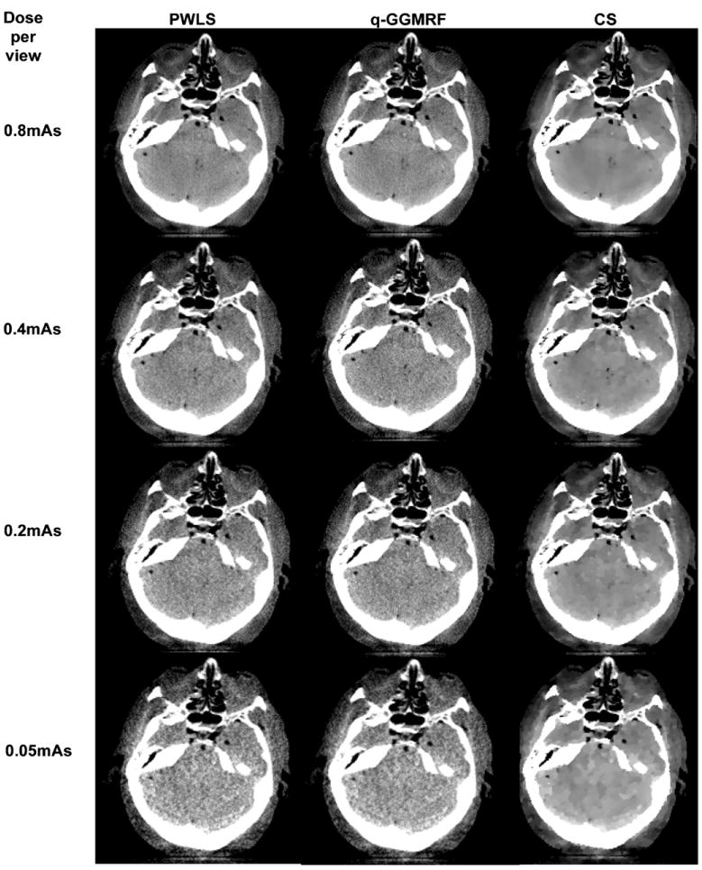
Reconstructions of different algorithms at different dose levels with 320 total views.

In order to further quantify the reconstruction accuracy for each algorithm, the RRME is calculated at different dose levels. The results are presented in figure 6. For all three algorithms, the RRME is well below 10% up to the dose level of 0.2 mAs/view. This result indicates that high reconstruction accuracy can be achieved when the iterative image reconstruction algorithms are utilized at low dose levels.

Figure 6.

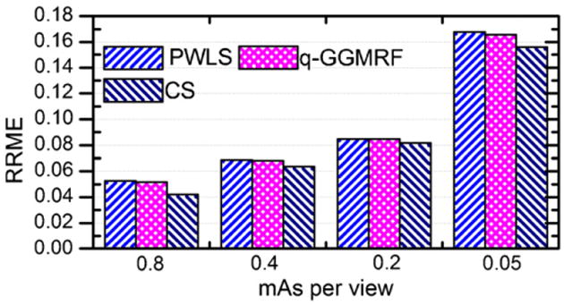
Reconstruction accuracy of the three algorithms at different dose levels.

Noise variances were also measured for the given ROI in figure 1. The results are given in figure 7. Clearly, the TV-based CS algorithm generates the lowest noise standard deviation at each of the dose levels. The other observation is that the standard deviations of the noise for both the PWLS and q-GGMRF algorithm increases with the decrease in the dose level while the noise standard deviation for the TV-based CS algorithm remains at a relative constant level.

Figure 7.

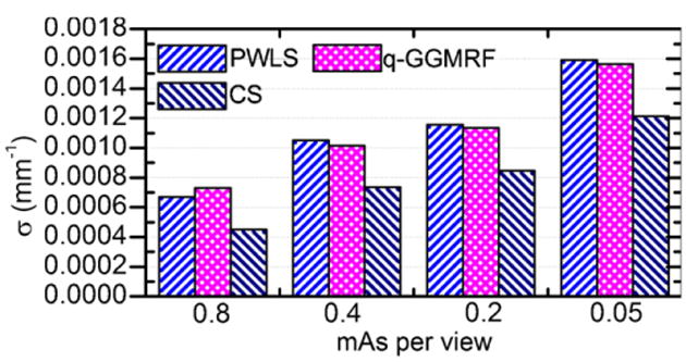
Noise standard deviations for the three algorithms at different dose levels.

For an unbiased comparison when we compare the noise level at each dose level, we must also evaluate the difference in spatial resolution for each algorithm. A sample MTF estimate is presented in figure 8. The result demonstrates that the TV-based CS algorithm has superior ability to reconstruct fine detailed high-contrast structures due to the edge-preservation feature in its regularization function.

Figure 8.

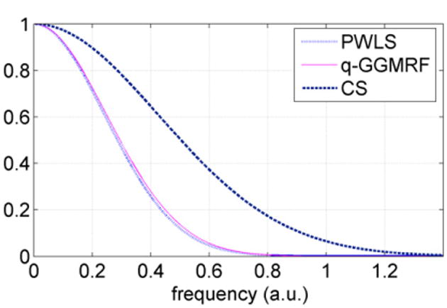
Estimated relative MTF for the three algorithms: PWLS, q-GGMRF and CS at 320 view angles and 0.8 mAs/view.

Using the estimated MTF curves and the variance measurements, the quality factor was calculated. In principle, the Q-factor may vary when different points on the MTF curve are used to define the characteristic spatial resolution. In this paper, for a relative comparison, the characteristic frequency values were taken where the MTF reached both 10% and 50% of the zero frequency value. As a result, the Q-factor values for the three algorithms at three different dose levels are given in figure 9. For each given algorithm, the quality factor decreases with a decrease in the radiation dose level. At each given dose level, the TV-based CS algorithm has the highest Q-factor value while the q-GGMRF algorithm is slightly superior to the PWLS algorithm. By comparing the Q-factor values at both 10% and 50% of the MTF curve, one can observe that the general conclusion is not dependent upon the specific characteristic spatial frequency chosen to define the spatial resolution.

Figure 9.

Comparison of Q-factor values for the three algorithms at different dose rates. Left: Q-factors calculated with a characteristic frequency of 50% of the MTF max. Right: Q-factors calculated with a characteristic frequency of 10% of the MTF max.

3.3. Algorithm performance comparison at a fixed total dose with varying view angle sampling

We have investigated the performance of the three algorithms at different sampling rates, and empirical lower bounds have been found for each algorithm in section 3.1. The investigation was conducted at a fixed dose per view angle. In reality, an interesting question of practical importance is the following, given a total radiation dose, what is the best manner to distribute the dose. Namely, is it better to deliver the dose to more view angles with a low mAs/view or is it better to distribute the total dose with a higher mAs/view. In the third study, the total radiation dose level was fixed at 64 mAs. Several different methods for distributing this total dose were used: (320 views, 20 mA, 10 ms), (160 views, 40 mA, 10 ms) and (80 views, 80 mA, 10 ms). The reconstructed images are presented in figure 10. In these images, significant streaking artifacts are present when the number of view angles is fewer than 320 views with the exception that the streaking artifacts in the CS image with 160 views are not significant. If we look through the columns, we can find for each algorithm that the image quality is better if the dose is delivered using more views. If we look though the rows, in the 320 views case, PWLS and q-GGMRF reconstructions provide visually better reconstruction results than the CS case as the CS image displays unphysical patchy artifacts. However, in the 160 views case, the CS reconstruction displays fewer streaking artifacts than the PWLS and q-GGMRF reconstructions.

Figure 10.

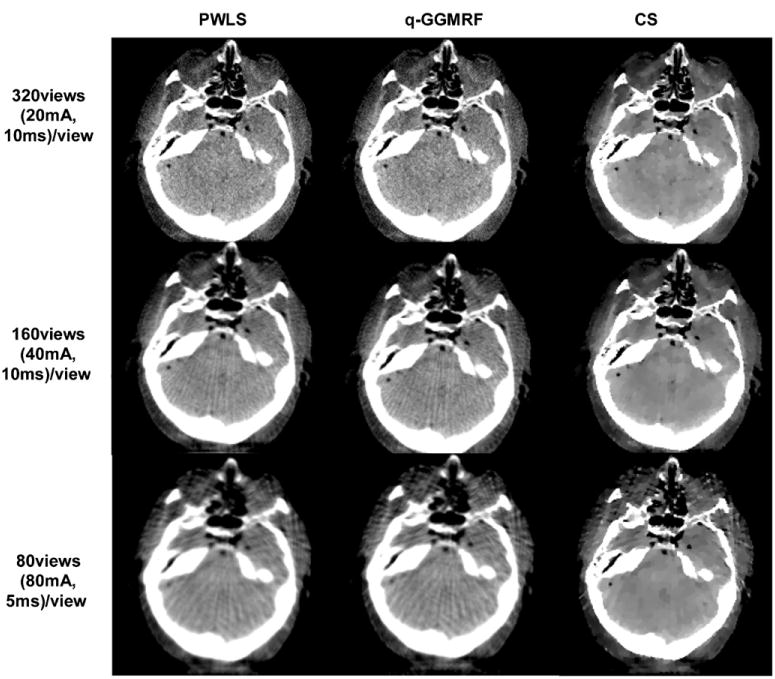
Reconstructed images at a fixed total dose at three different numbers of view angle, tube current and exposure time combinations.

A simple conclusion can be drawn from this study. Namely, one should distribute the total dose into many view angles with low mAs/view values provided that the corresponding projection noise level at low mAs/view values is not dominated by the electronic noise floor of the detector.

3.4. Control parameters β used in image reconstruction

As emphasized in section 2.4, the parameter β controls the strength of prior contribution. When the value of β is too large, images either become blurred (in the PWLS case) or become patchy (in the TV-based CS case). When β value is too small, the reconstructed images are either too noisy (PWLS) or too streaky (the TV-based CS case). In our image reconstruction procedure, the parameter was selected within a range of possible values. In figures 11, 12 and 13, the change of noise variance, spatial resolution and Q-factor for a representative experimental case (160 view angles and 0.8 mAs) are presented for the three image reconstruction algorithms. In order to plot all the curves in one figure, each parameter, i.e., noise, resolution and Q-factor, was normalized using the corresponding maximal values of the parameter. The β values which have been discarded due to excessive streaking (i.e. a high SI value) in the reconstructed images are circled.

Figure 11.

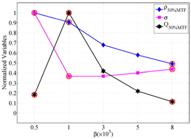
Selection of the β parameter for the quadratic PWLS algorithm.

Figure 12.

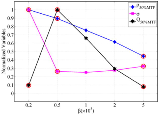
Selection of the β parameter for the q-GGMRF algorithm.

Figure 13.

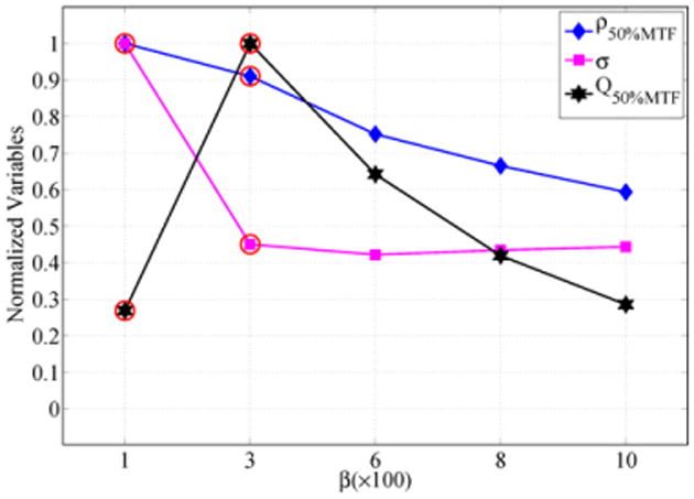
Selection of the β parameter for the TV-based algorithm.

In addition to the Q-factor versus β curve, we also presented the often used (Stayman and Fessler 2000, Wang et al 2006) noise-resolution tradeoff curve in figure 14. In a specific application, one can use this curve to guide the selection of β parameters for either better spatial resolution or better noise variance in image reconstruction.

Figure 14.

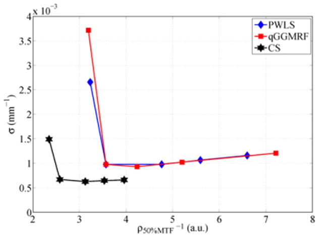
Noise-resolution tradeoff curve for the three algorithms: quadratic PWLS, q-GGMRF and TV-based CS.

For convenience, the values used for β in this work are also given in figures 15, 16 and 17 for the PWLS, q-GGMRF and TV-based CS algorithms at different view angle sampling rates and dose rates.

Figure 15.

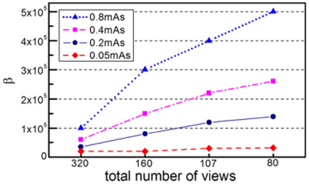
β parameters used in the PWLS algorithm at different dose rates and different view sampling rates.

Figure 16.

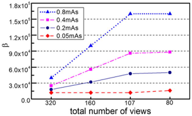
β parameters used in the q-GGMRF algorithm at different dose rates and different view sampling rates.

Figure 17.

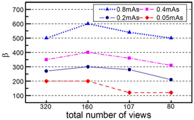
β parameters used in the TV-based CS algorithm at different dose rates and different view sampling rates.

For the PWLS algorithm, the reconstructed images become very streaky when the number of view angles is fewer than 100. For the case when more than 100 view angles are used, it was found that the selected values for β scale with the number of view angles in an approximately linear relation (figure 15). This linear relation between the β values and the view number is also valid for the q-GGMMRF algorithm (figure 16). However, the relationship changes for the TV-based CS algorithm. In this case, as shown in figure 17, larger values for β are needed for 160 views compared with 320 views to suppress streaking artifacts. However, when the number view angles are fewer than 160, the β values need to be decreased to prevent patchy artifacts in the reconstructed images.

4. Conclusions

In this paper, the performance of the TV-based CS algorithm is compared with other popular SIR algorithms such as the PWLS algorithm and the q-GGMRF algorithm. The comparison was conducted using experimental data acquired from a human cadaver head and an on-board cone-beam CT data acquisition system.

There are several important conclusions that can be drawn from this clinically realistic data set of a non-contrast-enhanced cadaver head. In the literature, CS has been reported to enable accurate reconstruction of the high-contrast Shepp–Logan numerical phantom from about 20 views of noise-free data. The experimental results in this study indicate that the CS algorithm performs better with respect to the streaking artifacts in the undersampling case than PWLS and q-GGMRF. However, the experimental results indicated that more than 100 views are still required to reconstruct images without streaking artifacts when realistic human anatomy is present. This result is consistent with the in vivo results of previous studies in both MRI (Block et al 2007, Lustig et al 2007, Gamper et al 2008, Jung et al 2009) and micro-CT (Song et al 2007). A second conclusion is that for a given dose level, superior image quality can be achieved by delivering the dose to more views with lower mAs per view than delivering it to fewer views with higher mAs per view, as long as the noise in each projection is quantum dominated. As expected the CS algorithm shows strong noise suppression characteristics. However, compared with other statistical algorithms, CS generates potentially misleading patchy structures when the total dose is very low.

The noise variance measurements, in principle, should be carried out by repeating the measurements many times and an ensemble average should be used. However, this experimental procedure will be very time consuming. Due to the limited availability of our clinical system for experimental data acquisition, we estimated the noise variance using the standard deviation of pixel values with essentially the same attenuation but distributed throughout the image. This method was selected as a standard ROI measurement is biased toward methods which encourage a high degree of spatial correlation such as the patchy artifacts in CS images. This measurement method must be considered when interpreting the results, as the results may be different than using the typical continuous ROI for measurement.

Currently, there is no single generally accepted figure of merit to comprehensively evaluate CT image quality. Limitations with the quality factor measurements made here include the fact that the noise standard deviation is not the only relevant parameter to assess low-contrast resolution performance (e.g. that the noise texture may also play a role). Therefore, in our future work, noise power spectrum studies will be performed to further evaluate the performance of various algorithms, and a comparison of the quality factors using multiple points on the MTF curves will be conducted. Additionally, since the quality factor is dependent upon the spatial resolution to the third power any change in the spatial resolution will greatly affect the quality factor. For this reason, since a high-contrast spatial resolution measurement was used here and the CS algorithm is excellent at preserving edges, the quality factor for the CS algorithm may be inflated. Thus, in figure 9, we do not suggest a direct comparison between different algorithms based on the quality factor Q, but rather a comparison within each algorithm as a function of dose. A new metric for overall image quality is needed to evaluate these nonlinear algorithms, which perhaps averages the spatial resolution at different contrast levels or penalizes the generation of patchy artifacts. In lieu of a new metric for overall image quality, task-based assessments using human and mathematical observers may be performed to evaluate each algorithm's utility for a given task.

References

- Andersen AH, Kak AC. Simultaneous algebraic reconstruction technique (Sart)—a superior implementation of the art algorithm. Ultrason Imag. 1984;6:81–94. doi: 10.1177/016173468400600107. [DOI] [PubMed] [Google Scholar]
- Beekman FJ, Kamphuis C. Ordered subset reconstruction for x-ray CT. Phys Med Biol. 2001;46:1835–44. doi: 10.1088/0031-9155/46/7/307. [DOI] [PubMed] [Google Scholar]
- Block KT, Uecker M, Frahm J. Undersampled radial MRI with multiple coils. Iterative image reconstruction using a total variation constraint. Magn Reson Med. 2007;57:1086–98. doi: 10.1002/mrm.21236. [DOI] [PubMed] [Google Scholar]
- Bouman C, Sauer K. A generalized Gaussian image model for edge-preserving MAP estimation. IEEE Trans Image Process. 1993;2:296–310. doi: 10.1109/83.236536. [DOI] [PubMed] [Google Scholar]
- Bouman CA, Sauer K. A unified approach to statistical tomography using coordinate descent optimization. IEEE Trans Image Process. 1996;5:480–92. doi: 10.1109/83.491321. [DOI] [PubMed] [Google Scholar]
- Brenner DJ, Hall EJ. Current concepts—computed tomography—an increasing source of radiation exposure. N Engl J Med. 2007;357:2277–84. doi: 10.1056/NEJMra072149. [DOI] [PubMed] [Google Scholar]
- Candes EJ, Romberg J, Tao T. Robust uncertainty principles: exact signal reconstruction from highly incomplete frequency information. IEEE Trans Inf Theory. 2006;52:489–509. [Google Scholar]
- Chen GH, Tang J, Hsieh J. Temporal resolution improvement using PICCS in MDCT cardiac imaging. Med Phys. 2009;36:2130–5. doi: 10.1118/1.3130018. [DOI] [PMC free article] [PubMed] [Google Scholar]
- Chen GH, Tang J, Leng S. Prior image constrained compressed sensing (PICCS): a method to accurately reconstruct dynamic CT images from highly undersampled projection data sets. Med Phys. 2008a;35:660–3. doi: 10.1118/1.2836423. [DOI] [PMC free article] [PubMed] [Google Scholar]
- Chen GH, Tang J, Leng S. Prior image constrained compressed sensing (PICCS) Proc SPIE. 2008b;6856:685618. doi: 10.1117/12.770532. [DOI] [PMC free article] [PubMed] [Google Scholar]
- Combettes PL, Pesquet JC. Image restoration subject to a total variation constraint. IEEE Trans Image Process. 2004;13:1213–22. doi: 10.1109/tip.2004.832922. [DOI] [PubMed] [Google Scholar]
- De Man B, et al. Metal streak artifacts in x-ray computed tomography: a simulation study. IEEE Trans Nucl Sci. 1999;46:691–6. [Google Scholar]
- De Man B, et al. Reduction of metal streak artifacts in x-ray computed tomography using a transmission maximum a posteriori algorithm. IEEE Trans Nucl Sci. 2000;47:977–81. [Google Scholar]
- De Man B, et al. An iterative maximum-likelihood polychromatic algorithm for CT. IEEE Trans Med Imag. 2001;20:999–1008. doi: 10.1109/42.959297. [DOI] [PubMed] [Google Scholar]
- De Man B, et al. A study of four minimization approaches for iterative reconstruction in x-ray CT. Nuclear Science Symp Conf Record (2005 IEEE) 2005 [Google Scholar]
- Dempster AP, Laird NM, Rubin DB. Maximum likelihood from incomplete data via EM algorithm. J R Stat Soc Ser B-Methodol. 1977;39:1–38. [Google Scholar]
- Donoho DL. Compressed sensing. IEEE Trans Inf Theory. 2006;52:1289–306. [Google Scholar]
- Elbakri IA, Fessler JA. Statistical image reconstruction for polyenergetic x-ray computed tomography. IEEE Trans Med Imag. 2002;21:89–99. doi: 10.1109/42.993128. [DOI] [PubMed] [Google Scholar]
- Erdogan H, Fessler JA. Ordered subsets algorithms for transmission tomography. Phys Med Biol. 1999;44:2835–51. doi: 10.1088/0031-9155/44/11/311. [DOI] [PubMed] [Google Scholar]
- Fessler JA, Hero AO. Penalized maximum-likelihood image-reconstruction using space-alternating generalized EM algorithms. IEEE Trans Image Process. 1994;4:1417–29. doi: 10.1109/83.465106. [DOI] [PubMed] [Google Scholar]
- Gamper U, Boesiger P, Kozerke S. Compressed sensing in dynamic MRI. Magn Reson Med. 2008;59:365–73. doi: 10.1002/mrm.21477. [DOI] [PubMed] [Google Scholar]
- Geman D, McClure DE. Bayesian image analysis: an application to single photon emission tomography. Proc Stat Comput Section Amer Stat Assoc 1985 [Google Scholar]
- Geman S, McClure DE, Geman D. A nonlinear filter for film restoration and other problems in image-processing. CVGIP, Graph Models Image Process. 1992;54:281–9. [Google Scholar]
- Geman D, Reynolds G. Constrained restoration and the recovery of discontinuities. IEEE Trans Pattern Anal Mach Intell. 1992;14:367–83. [Google Scholar]
- Geman D, Yang CD. Nonlinear image recovery with half-quadratic regularization. IEEE Trans Image Process. 1995;4:932–46. doi: 10.1109/83.392335. [DOI] [PubMed] [Google Scholar]
- Geman D, et al. Boundary detection by constrained optimization. IEEE Trans Pattern Anal Mach Intell. 1990;12:609–28. [Google Scholar]
- Gilbert P. Iterative methods for 3-dimensional reconstruction of an object from projections. J Theor Biol. 1972;36:105–7. doi: 10.1016/0022-5193(72)90180-4. [DOI] [PubMed] [Google Scholar]
- Gordon R, Bender R, Herman GT. Algebraic reconstruction techniques (Art) for 3-dimensional electron microscopy and x-ray photography. J Theor Biol. 1970;29:471–81. doi: 10.1016/0022-5193(70)90109-8. [DOI] [PubMed] [Google Scholar]
- Gordon R, Herman GT. 3-Dimensional reconstruction from projections—review of algorithms. Int Rev Cytol. 1974;38:111–51. doi: 10.1016/s0074-7696(08)60925-0. [DOI] [PubMed] [Google Scholar]
- Green PJ. Bayesian reconstructions from emission tomography data using a modified EM algorithm. IEEE Trans Med Imag. 1990;9:84–93. doi: 10.1109/42.52985. [DOI] [PubMed] [Google Scholar]
- Herman GT. Image Reconstruction from Projections: The Fundamentals of Computerized Tomography. San Francisco, CA: Academic; 1980. [Google Scholar]
- Herman GT, Davidi R. Image reconstruction from a small number of projections. Inverse Problems. 2008;24:040511. doi: 10.1088/0266-5611/24/4/045011. [DOI] [PMC free article] [PubMed] [Google Scholar]
- Hounsfield CN. A method of and apparatus for examination of a body by radiation such as x or gamma radiation. Patent Specification. 1968:1283915. [Google Scholar]
- Hsieh J. Adaptive streak artifact reduction in computed tomography resulting from excessive x-ray photon noise. Med Phys. 1998;25:2139–47. doi: 10.1118/1.598410. [DOI] [PubMed] [Google Scholar]
- Hsieh J. Computed Tomography: Principles, Design, Artifacts, and Recent Advances. Bellingham, WA: SPIE Optical Engineering Press; 2003. [Google Scholar]
- Hudson HM, Larkin RS. Accelerated image-reconstruction using ordered subsets of projection data. IEEE Trans Med Imag. 1994;13:601–9. doi: 10.1109/42.363108. [DOI] [PubMed] [Google Scholar]
- Jiang M, Wang G. Convergence of the simultaneous algebraic reconstruction technique (SART) IEEE Trans Image Process. 2003a;12:957–61. doi: 10.1109/TIP.2003.815295. [DOI] [PubMed] [Google Scholar]
- Jiang M, Wang G. Convergence studies on iterative algorithms for image reconstruction. IEEE Trans Med Imag. 2003b;22:569–79. doi: 10.1109/TMI.2003.812253. [DOI] [PubMed] [Google Scholar]
- Jung H, et al. k-t FOCUSS: a general compressed sensing framework for high resolution dynamic MRI. Magn Reson Med. 2009;61:103–16. doi: 10.1002/mrm.21757. [DOI] [PubMed] [Google Scholar]
- Kachelriess M, Berkus T, Kalender W. Quality of statistical reconstruction in medical CT. Nuclear Science Symp Conf Record (2003 IEEE) 2003 [Google Scholar]
- Kak AC, Slaney M. Principles of Computerized Tomographic Imaging. Philadelphia, PA: SIAM Press; 2001. [Google Scholar]
- Kolehmainen V, et al. Statistical inversion for medical x-ray tomography with few radiographs: II. Application to dental radiology. Phys Med Biol. 2003;48:1465–90. doi: 10.1088/0031-9155/48/10/315. [DOI] [PubMed] [Google Scholar]
- Kalender WA. Computed Tomography: Fundamentals, System Technology, Image Quality, Applications. 2nd. Erlangen: Publicis Corporate Publishing; 2005. [Google Scholar]
- Kawata S, Nalcioglu O. Constrained iterative reconstruction by the conjugate-gradient method. IEEE Trans Med Imag. 1985;4:65–71. doi: 10.1109/TMI.1985.4307698. [DOI] [PubMed] [Google Scholar]
- Lange K, Carson R. EM reconstruction algorithms for emission and transmission tomography. J Comput Assist Tomogr. 1984;8:306–16. [PubMed] [Google Scholar]
- Lange K, Fessler JA. Globally convergent algorithms for maximum a-posteriori transmission tomography. IEEE Trans Image Process. 1995;4:1430–8. doi: 10.1109/83.465107. [DOI] [PubMed] [Google Scholar]
- Leng S, et al. High temporal resolution and streak-free four-dimensional cone-beam computed tomography. Phys Med Biol. 2008;53:5653–73. doi: 10.1088/0031-9155/53/20/006. [DOI] [PMC free article] [PubMed] [Google Scholar]
- Li MH, Yang HQ, Kudo H. An accurate iterative reconstruction algorithm for sparse objects: application to 3D blood vessel reconstruction from a limited number of projections. Phys Med Biol. 2002;47:2599–609. doi: 10.1088/0031-9155/47/15/303. [DOI] [PubMed] [Google Scholar]
- Li T, et al. Radiation dose reduction in four-dimensional computed tomography. Med Phys. 2005;32:3650–60. doi: 10.1118/1.2122567. [DOI] [PubMed] [Google Scholar]
- Lustig M, Donoho D, Pauly JM. Sparse MRI: the application of compressed sensing for rapid MR imaging. Magn Reson Med. 2007;58:1182–95. doi: 10.1002/mrm.21391. [DOI] [PubMed] [Google Scholar]
- Panin VY, Zeng GL, Gullberg GT. Total variation regulated EM algorithm. IEEE Trans Nucl Sci. 1999;46:2202–10. [Google Scholar]
- Persson M, Bone D, Elmqvist H. Total variation norm for three-dimensional iterative reconstruction in limited view angle tomography. Phys Med Biol. 2001;46:853–66. doi: 10.1088/0031-9155/46/3/318. [DOI] [PubMed] [Google Scholar]
- Rockmore AJ, Macovski A. Maximum likelihood approach to emission image-reconstruction from projections. IEEE Trans Nucl Sci. 1976;23:1428–32. [Google Scholar]
- Rockmore AJ, Macovski A. Maximum likelihood approach to transmission image-reconstruction from projections. IEEE Trans Nucl Sci. 1977;24:1929–35. [Google Scholar]
- Rudin LI, Osher S, Fatemi E. Nonlinear total variation based noise removal algorithms. Physica D. 1992;60:259–68. [Google Scholar]
- Sauer K, Bouman C. A local update strategy for iterative reconstruction from projections. IEEE Trans Signal Process. 1993;41:534–48. [Google Scholar]
- Shepp LA, Vardi Y. Maximum likelihood reconstruction for emission tomography. Med Imag IEEE Trans. 1982;1:113–22. doi: 10.1109/TMI.1982.4307558. [DOI] [PubMed] [Google Scholar]
- Sidky EY, Kao CM, Pan XH. Accurate image reconstruction from few-views and limited-angle data in divergent-beam CT. J X-Ray Sci Technol. 2006;14:119–39. [Google Scholar]
- Sidky EY, Pan XC. Image reconstruction in circular cone-beam computed tomography by constrained, total-variation minimization. Phys Med Biol. 2008;53:4777–807. doi: 10.1088/0031-9155/53/17/021. [DOI] [PMC free article] [PubMed] [Google Scholar]
- Song J, et al. Sparseness prior based iterative image reconstruction for retrospectively gated cardiac micro-CT. Med Phys. 2007;34:4476–83. doi: 10.1118/1.2795830. [DOI] [PMC free article] [PubMed] [Google Scholar]
- Stayman JW, Fessler JA. Regularization for uniform spatial resolution properties in penalized-likelihood image reconstruction. IEEE Trans Med Imag. 2000;19:601–15. doi: 10.1109/42.870666. [DOI] [PubMed] [Google Scholar]
- Sukovic P, Clinthorne NH. Penalized weighted least-squares image reconstruction for dual energy x-ray transmission tomography. IEEE Trans Med Imag. 2000;19:1075–81. doi: 10.1109/42.896783. [DOI] [PubMed] [Google Scholar]
- Thibault JB, et al. A three-dimensional statistical approach to improved image quality for multislice helical CT. Med Phys. 2007;34:4526–44. doi: 10.1118/1.2789499. [DOI] [PubMed] [Google Scholar]
- Velikina J, Leng S, Chen GH. Limited view angle tomographic image reconstruction via total variation minimization. SPIE Proc Med Imaging. 2007;6510:651020. [Google Scholar]
- Wang G, et al. Iterative deblurring for CT metal artifact reduction. IEEE Trans Med Imag. 1996;15:657–64. doi: 10.1109/42.538943. [DOI] [PubMed] [Google Scholar]
- Wang J, et al. Penalized weighted least-squares approach to sinogram noise reduction and image reconstruction for low-dose x-ray computed tomography. IEEE Trans Med Imag. 2006;25:1272–83. doi: 10.1109/42.896783. [DOI] [PMC free article] [PubMed] [Google Scholar]
- Wang J, et al. Dose reduction for kilovotage cone-beam computed tomography in radiation therapy. Phys Med Biol. 2008;53:2897–909. doi: 10.1088/0031-9155/53/11/009. [DOI] [PubMed] [Google Scholar]
- Wang J, Li TF, Xing L. Iterative image reconstruction for CBCT using edge-preserving prior. Med Phys. 2009;36:252–60. doi: 10.1118/1.3036112. [DOI] [PMC free article] [PubMed] [Google Scholar]
- Wang G, Snyder DL, Vannier MW. Iterative deblurring of CT image-restoration, metal artifact reduction and local reconstruction. Radiology. 1995;197:291–1. [Google Scholar]
- Yu H, Wang G. Compressed sensing based interior tomography. Phys Med Biol. 2009;54:2791–805. doi: 10.1088/0031-9155/54/9/014. [DOI] [PMC free article] [PubMed] [Google Scholar]
- Zbijewski W, et al. Statistical reconstruction for x-ray CT systems with non-continuous detectors. Phys Med Biol. 2007;52:403–18. doi: 10.1088/0031-9155/52/2/007. [DOI] [PubMed] [Google Scholar]