Measurement of the spatial backscattering impulse-response at short length-scales with polarized enhanced backscattering (EBS)

Abstract

In this Letter, we describe an easy to implement technique to measure the spatial backscattering impulse-response at length-scales shorter than a transport mean free path with resolution of better than 10 μm using the enhanced backscattering (EBS) phenomenon. This technique enables spectroscopic measurements throughout the visible range and sensitivity to all polarization channels. Through a combination of Monte Carlo simulations and experimental measurements of latex microspheres, we explore the various sensitivities of our technique to both intrinsic sample properties and extrinsic instrumental properties. We conclude by demonstrating the extraordinary sensitivity of our technique to the shape of the scattering phase function, including higher order shape parameters than the anisotropy factor (or first moment).

The spatial backscattering impulse-response at length-scales shorter than a transport mean free path $l_s^{\ast }$ is highly sensitive to the shape of the scattering phase function due to the fact that rays exiting within this regime have undergone relatively few scattering events. Typically this measurement is accomplished using a lens to focus the illumination beam to a near impulse on the sample surface. A CCD camera then detects the spatial distribution of backscattered light at the sample surface. With this design, the full azimuthal backscattering distribution can easily be measured for each polarization channel [1]. Still, a true impulse can never be achieved and information at short length-scales is lost to an optical mask (~mm diameter) needed to reject specular reflections. Thus in media such as biological tissue with long $l_s^{\ast }$ on the order of 1 mm, information about the shape of the phase function is extremely difficult to measure experimentally. As an alternative to overcome these difficulties, here we report a simple bench-top instrument using polarized enhanced backscattering (EBS) to first measure the backscattering distribution in the angular domain and subsequently convert to the spatial domain through inverse Fourier transformation.

EBS is an angular intensity peak centered in the exact backscattering direction that is formed by the summed diffraction pattern from all sets of time-reversed path-pairs within a scattering medium (a direct consequence of the reciprocity theorem) [2]. Conceptually, it is useful to think of each time-reversed path-pair as a single Young’s double pinhole experiment. For a single time-reversed path-pair with rays exiting at a particular spatial separation, the diffraction pattern is the Fourier transform of two delta functions (cosine pattern). For a semi-infinite medium under plane wave illumination the distribution of spatial separations for all time-reversed path-pairs is given by the spatial backscattering impulse-response for multiply scattered light in the exact backward direction p(x,y). As a result, in an idealized case the EBS peak I_EBS(θ_x, θ_y) is simply the Fourier transform of p(x,y). However, as we will demonstrate the dependencies are more complex:

$$I_{\mathit{EBS}}({\theta }_x,{\theta }_y)=ℱ\{p(x,y)·\mathit{pc}(x,y)·s(x,y)·c(x,y)·\mathit{mtf}(x,y)\},$$ (1)

where ℱ denotes the Fourier transform operation, pc specifies the degree of phase correlation between the forward and reverse path, s represents the effective distribution of rays which remain within the illumination spot, c is the spatial coherence function, and mtf is the modulation transfer function of the optical instrument. Within the ℱ operation, p and pc represent instrinsic sample properties while s, c, and mtf represent extrinsic instrument properties. Each of these functions will described in further detail in the following paragraphs.

The experimentally measurable p_eff is found by computing the inverse Fourier transform of the EBS peak:

$$p_{\mathit{eff}}={ℱ}^{-1}\{I_{\mathit{EBS}}({\theta }_x,{\theta }_y)\},$$ (2)

For sample characterization, the functions p and pc are of prime interest. In principle these intrinsic parameters can be found by dividing p_eff by functions s, c, and mtf. However, in practice this will amplify noise and a reliable result can be difficult to obtain. Alternatively, a more stable approach which we follow in this Letter is to convert theory into the experimentally observable p_eff before comparison with experiment.

Our experimental instrument is shown in Fig. 1. An illumination source (xenon lamp with finite spatial coherence length L_sc or broadband laser with L_sc = ∞) is collimated by lens L₁ and polarized by linear polarizer P before being directed onto the scattering sample via a non-polarizing 50/50 beam splitter B. Backscattered light is then collected by B and passes through a linear analyzer A before being focused onto a CCD camera with a lens L₂. A liquid crystal tunable filter attached to the CCD separates the backscattered light into its component wavelengths. All polarization combinations are achieved by rotating P and/or inserting a quarter wave plate QWP between B and the sample.

Fig. 1.

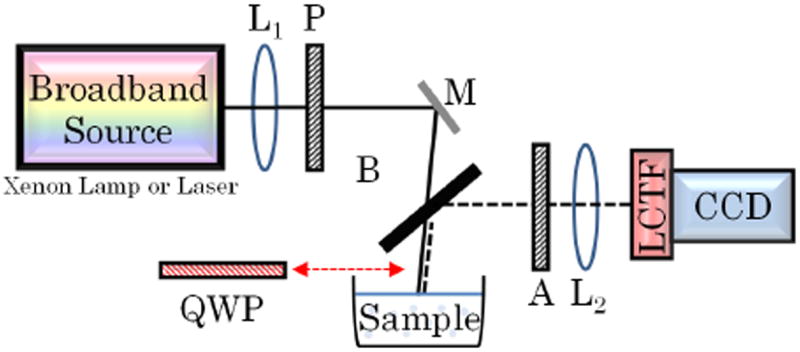
EBS instrument. Collimating lens L₁ (f = 200 mm), linear polarizer P, mirror M, beam splitter B, quarter wave plate QWP, linear analyzer A, Fourier lens L₂ (f = 100 mm), liquid crystal tunable filter LCTF.

Information regarding the processing of experimental and Monte Carlo simulated EBS data can be found in detail in other publications [3,4]. It should be noted that all experimental data is scaled by a constant multiplicative factor of 0.65 to obtain a full match with Monte Carlo simulation [4]. This type of one parameter fit is common in EBS literature [5]. In this Letter, all experiments and Monte Carlo simulations are for aqueous latex microsphere suspensions (10% solids by weight) which are diluted in DI water to achieve different values of $l_s^{\ast }$ After retrieving the experimental EBS peak, the spatial distribution of backscattered light is computed using Eq. 2. According to the properties of the discrete Fourier transform, the spatial resolution Δs is related to the angular resolution Δθ by:

$$\mathrm{\Delta }s=\frac{\mathrm{\lambda }}{n·\mathrm{\Delta }\theta },$$ (3)

where λ is the illumination wavelength and n is the number of pixels in the x or y direction. Our instrument collects angles up to 7.5776° with 0.0074° resolution. Within the visible range of illumination this corresponds to a spatial extent of >1500 μm with <10 μm resolution.

Strictly speaking the reciprocity theorem is only fully valid for polarization preserving channels (i.e. linear co-polarized xx or helicity preserving ++) [2]. For these channels, each ray has a time-reversed partner which exits with the same accumulated phase and pc = 1 for all x,y positions. However, in the orthogonal polarization channels (i.e. linear cross-polarized xy or opposite helicity +-) not all scattering rotations are reversible. As a result, the forward and reverse paths may exit with different phases and pc does not necessarily equal 1. Following the calculations of Ref. [6], pc in the orthogonal channels can be approximated from the degree of linear ( $\mathit{dlp}=\frac{(\mathit{xx})-(\mathit{xy})}{(\mathit{xx})+(\mathit{xy})}$) and circular ( $\mathit{dcp}=\frac{(++)-(+-)}{(++)+(+-)}$) polarization:

$$\begin{array}{lll}{\mathit{pc}}_{\mathit{xy}}(r)& =& \frac{\mathit{dlp}(r)+\mathit{dcp}(r)}{1-\mathit{dlp}(r)}\\ {\mathit{pc}}_{+-(r)}& =& \frac{2·\mathit{dlp}(r)}{1-\mathit{dcp}(r)}\end{array}$$ (4)

Figure 2a shows function pc for the four measured polarization channels. For very short length-scales, rays undergo relatively few scattering events and pc is nearly 1. As the exit radius increases, the average number of scattering events also increases. As a result, a greater proportion of rays travel through irreversible paths and pc → 0 as r → ∞ [2]. Figure 2b shows the excellent agreement between experiment and simulation for p_eff measured from each of the 4 polarization channels.

Fig. 2.

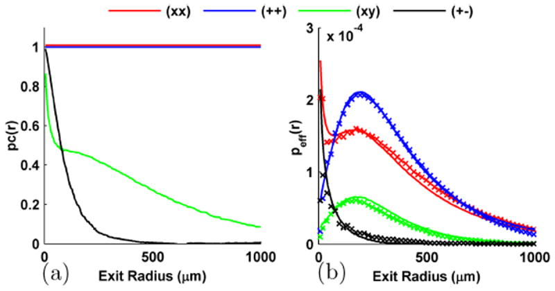
Polarization sensitivities. (a) Function pc for the 4 measured polarization channels as a function of exit radius. (b) Experimental (symbols) and simulation (lines) p_eff. Sample : 0.65μm diameter sphere with $l_s^{\ast }$ = 205 μm at 633 nm. Spot size = 6000 μm and L_sc = ∞. Simulation scaled by 0.65 to obtain match with experiment.

Since realistic experiments have finite illumination beam extent, an effective distribution of rays which remain within the illumination spot (and therefore possess a time-reversed partner) must be found. This can be obtained by computing the normalized autocorrelation function ACF of the illumination pattern A incident on the scattering sample [4]:

$$s(x,y)=\mathit{ACF}\{A(x,y)\},$$ (5)

In our case, a circular beam is used and A is a top hat function (i.e. A = 1 within the illumination spot and 0 otherwise). For each spot size, s begins at 1 and decreases to 0 when the path-pair separation is larger than the beam diameter. Figure 3a shows function s for 2 illumination spot sizes. Figure 3b shows excellent agreement between the experiment and simulation p_eff for 2000 and 7000 μm spot sizes.

Fig. 3.

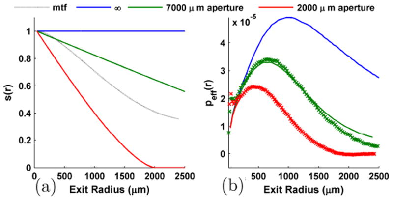
Illumination beam spot size sensitivities. (a) s as a function of exit radius for 2 beam spot sizes. (b) Comparison between experiment (symbols) and simulation (lines) for the different beam spot sizes using ++ polarization. Sample : 0.65 μm diameter sphere with $l_s^{\ast }$ = 950 μm at 633 nm. L_sc = ∞. Simulation scaled by 0.65.

Another consideration for the measurement of p_eff is function c which describes the ability for path-pairs to interfere when using a partial spatial coherence source. For a typical laser source, L_sc is sufficiently large that over the extent of the beam spot size it can be considered spatially coherent (i.e. c = 1). However, even for illumination with very short L_sc (e.g. sunlight or xenon source) an EBS peak is formed. In this case, function c can be found according to the van-Cittert Zernike theorem. For our instrument, function c takes the form of a first-order Bessel function of the first kind J₁ [3].

$$c(r)=\frac{2J_1\left(r/L_{\mathit{sc}}\right)}{r/L_{\mathit{sc}}},$$ (6)

Figure 4a shows function c for illumination with 4 different L_sc possible with our instrument. Figure 4b shows the agreement between the experiment and simulation p_eff for each of these L_sc.

Fig. 4.

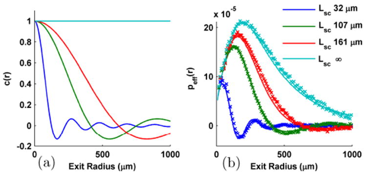
Sensitivities to the spatial coherence of the illumination. (a) Function c for different L_sc. (b) Comparison between experiment (symbols) and simulation (lines) for different L_sc using ++ polarization. Sample : 0.65 μm diameter sphere with $l_s^{\ast }$ = 205 μm at 633 nm. Spot size = 6000 μm and L_sc = ∞. Simulation scaled by 0.65.

For any imaging system the mtf describes the ability to capture information from different spatial frequencies. As such, the measurement of p_eff will also be modulated by the mtf. To determine our system’s mtf (shown in Fig. 3a) we computed the Fourier transform of the point spread function measured by placing a mirror in the sample plane and imaging the laser onto the CCD.

As a final demonstration of the sensitivity of our technique to fine details in the scattering phase function, we measure two suspensions of microspheres with the same $l_s^{\ast }$ (1000 μm) and anisotropy factor g (0.87) but different size parameter ka (where k is the wavenumber in water and a is the microsphere radius). Figure 5a displays the two samples’ phase functions. Although they are generally similar in shape, the sample with higher ka has many higher frequency oscillations in accordance with Mie theory. In Fig. 5b we demonstrate that these higher frequency oscillations have a profound effect on the shape of p_eff at short length-scales. These slight differences are readily distinguishable using the technique presented in this Letter.

Fig. 5.

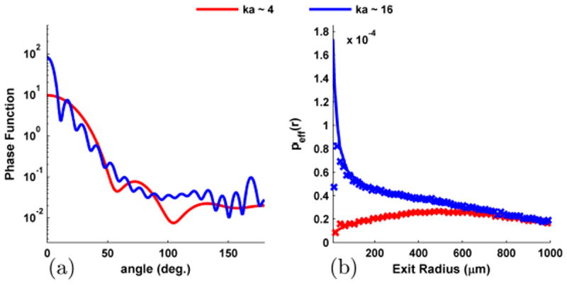
Sensitivity of EBS to the phase function. (a) Phase function for two microsphere samples with the same g but different ka. (b) Corresponding p_eff for ++ polarization shows a large difference in shape at short length-scales. ka ~ 4 : 0.65 μm diameter sphere at 633 nm. ka ~ 16 : 2.1 μm diameter sphere at 558 nm. Spot size = 2000 μm and L_sc = ∞. Simulation scaled by 0.65.

In summary we have presented EBS as a useful method to measure the backscattering impulse-response at small length-scales where information about the phase function is preserved. We first discussed the various sample dependent and experimental variables which affect the measurement and then provided a demonstration of its extraordinary sensitivity to the shape of the phase function.

References

- 1.Hielscher A, Eick A, Mourant J, Shen D, Freyer J, Bigio I. Diffuse backscattering Mueller matrices of highly scattering media. Optic Express. 1997;1:441–453. doi: 10.1364/oe.1.000441. [DOI] [PubMed] [Google Scholar]
- 2.Lenke R, Maret G. Multiple scattering of light:coherent backscattering and transmission. In: Brown W, Mortensen K, editors. Scattering in Polymeric and Colloidal Systems. 2000. [Google Scholar]
- 3.Turzhitsky V, Rogers JD, Mutyal NN, Roy HK, Backman V. Characterization of light transport in scattering media at subdiffusion length scales with low-coherence enhanced backscattering. IEEE Journal of Selected Topics in Quantum Electronics. 2010;16:619–626. doi: 10.1109/JSTQE.2009.2032666. [DOI] [PMC free article] [PubMed] [Google Scholar]
- 4.Radosevich AJ, Rogers JD, Turzhitsky V, Mutyal NN, Yi J, Roy HK, Backman V. Polarized enhanced backscattering spectroscopy for characterization of biological tissues at subdiffusion length-scales. IEEE J Sel Top Quantum Electron (2012) 2011 Oct 20; doi: 10.1109/JSTQE.2011.2173659. doc. ID JSTQE-INV-BIO2-04246-2011, in press. [DOI] [PMC free article] [PubMed] [Google Scholar]
- 5.Ospeck M, Fraden S. Influence of reflecting boundaries and finite interfacial thickness on the coherent backscattering cone. Phys Rev E. 1994;49:4578. doi: 10.1103/physreve.49.4578. [DOI] [PubMed] [Google Scholar]
- 6.Lenke R, Maret G. Magnetic field effects on coherent backscattering of light. European Physical Journal B. 2000;17:171–185. [Google Scholar]