PHYLOSEQ: A BIOCONDUCTOR PACKAGE FOR HANDLING AND ANALYSIS OF HIGH-THROUGHPUT PHYLOGENETIC SEQUENCE DATA

Abstract

We present a detailed description of a new Bioconductor package, phyloseq, for integrated data and analysis of taxonomically-clustered phylogenetic sequencing data in conjunction with related data types. The phyloseq package integrates abundance data, phylogenetic information and covariates so that exploratory transformations, plots, and confirmatory testing and diagnostic plots can be carried out seamlessly. The package is built following the S4 object-oriented framework of the R language so that once the data have been input the user can easily transform, plot and analyze the data. We present some examples that highlight the methods and the ease with which we can leverage existing packages.

1. Introduction

High-throughput (HT) DNA sequencing¹ is allowing major advances in microbial ecology studies,² where our understanding of the presence and abundance of microbial species relies heavily on the observation of their nucleic acids in a “culture independent” manner.³ Typically this is achieved by PCR amplification of a small ( 100–500 bp) fragment of a conserved gene (phylogenetic marker) for which there are taxonomically-informative reference sequences available. The most commonly-used phylogenetic marker gene is the small subunit ribosomal RNA (16S rRNA) gene,³ for which there are also convenient tools⁴ and large reference databases.^5–7

The first step in interpreting this phylogenetic sequencing data is usually to define a species-equivalent operational taxonomic unit (OTU). Species clustering methods are a separate area of research^8,9 beyond the scope of this article, but there are several packages/pipelines currently available to perform processing of raw HT phylogenetic sequencing data such that sequences are both clustered and the clusters are classified taxonomically. These include QI-IME,¹⁰ mothur,¹¹ the RDP pipeline⁶ and PANGEA.^12a In some cases these applications are also able to perform downstream analyses, but the options are limited. While there may be some anecdotal advantages to having a downstream ecological analysis coupled with the application that defined the OTUs, we expect that they are outweighed by the advantages of a separate set of flexible, open-source analyses that can be applied consistently across experiments, independent of the choice of OTU clustering method. There are already several ecology and phylogenetic packages available in R, including the adephylo,¹³ vegan,¹⁴ ade4 ,¹⁵ picante,¹⁶ ape,¹⁷ phangorn,¹⁸ phylobase,¹⁹ and OTUbase²⁰ packages, and these can already take advantage of many of the powerful statistical and graphics tools available in R.²¹ However, at present a user must devise their own methods for parsing the output of their favorite OTU clustering application, and, as a consequence, there is also no standard within Bioconductor²² (or R generally) for storing or sharing the suite of related data objects that describe a phylogenetic sequencing project.

To address these issues, we have created a new package for Bioconductor, called phyloseq, that provides a related set of S4 classes²³ that internally manage the handling tasks associated with organizing, linking, and storing phylogenetic sequencing data. The user is able to store all their relevant data types in a single phyloseq object. This approach has several advantages. First, it is easier to return to a previously-analyzed dataset, because the data is organized by design. Secondly, this data structure and accompanied methods make it is easier to share/compare data from separate experiments, as well as apply a consistent set of analysis methods to multiple experiments. For development, new method extensions can be created that recognize exactly the data types that are present in a particular phyloseq class. To in-stantiate an object of the appropriate phyloseq class, the user calls the initialization method (phyloseq(…)) with available core data types as input. Alternatively, the phyloseq package contains data input methods for each of the four main OTU clustering applications described above, allowing the user to import their data and check its compatibility in one function call.

The phyloseq package also allows the modification and subsetting of phyloseq objects, such that the component data types remain compatible at every step (e.g. contain exactly the same samples and taxa) and component data is easily accessed. Furthermore, the phyloseq package contains convenient wrapper methods for executing common analysis pipelines and creating useful graphics. Also provided are parallelized methods (using Rmpi²⁴) for calculating the UniFrac²⁵ and weighted-UniFrac²⁶ distances — common methods for calculating the relative dissimilarities of the microbial communities of different samples. Parallelization of these two methods is especially important because they are computationally intensive calculations for experiments with a large number of diverse samples. If alternatively a user wants to off-load the UniFrac calculation to the UniFrac server,²⁷ phyloseq provides an export method that creates the required environment and NEXUS files directly from the abundance table and phylogenetic tree, respectively. Finally, we expect that the S4 data structure and core object handling methods in the phyloseq package will facilitate development of novel methods and classes for phylogenetic sequencing analysis.

A related Bioconductor package, OTUbase,²⁰ currently allows for importing output from the mothur pipeline and retaining metadata associated with the raw HT sequencing, for example the read labels and sequence quality of individual reads. The phyloseq package provides some useful importing methods to support users that have already imported mothur datasets using OTUbase.

2. Class Structure

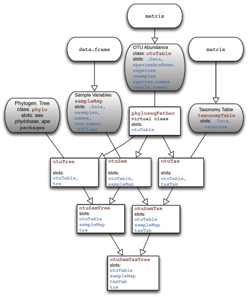
The class structure in the phyloseq package follows the inheritance diagram shown in Fig. 1. The phyloseq package contains multiple inherited classes with incremental complexity so that methods can be extended to handle exactly the data types that are present in a particular object. Currently, phyloseq uses 4 core data classes. They are the taxonomic abundance table (otuTable), a table of sample data (sampleMap), a table of taxonomic descriptors (taxonomyTable), and a phylogenetic tree (phylo) which is directly borrowed from the phylobase and ape packages. The otuTable class can be considered the central data type, as it directly represents the number and type of sequences observed in each sample. otuTable extends the numeric matrix class in the R base, and has a few additonal feature slots. The most important of these feature slots is the speciesAreRows slot, which holds a single logical that indicates whether the table is oriented with taxa as rows (as in the genefilter package in Bioconductor²²) or with taxa as columns (as in vegan and picante packages). In phyloseq methods, as well as its extensions of methods in other packages, the speciesAreRows value is checked to ensure proper orientation of the otuTable. A phyloseq user is only required to specify the otuTable orientation during initialization, following which all handling is internal.

Fig. 1.

Classes and inheritance in the phyloseq package. Core data classes are shown with grey fill and rounded corners. The class name and its slots are shown with red- or blue-shaded text, respectively. Inheritance is indicated graphically by arrows. Lines without arrows indicate that a higher-order object contains a slot with the associated class as one of its components.

The sampleMap class directly inherits R’s data.frame class, and thus effectively stores both categorical and numerical data about each sample. The orientation of a data.frame in this context requires that samples/trials are rows, and variables are columns (consistent with vegan and other packages). The taxonomyTable class directly inherits the matrix class, and is oriented such that rows are taxa (e.g. species) and columns are taxonomic ranks (e.g. phylum).

We use the term “higher-order classes” for those that contain two or more of the previously-described core data classes. We assume that phyloseq users will be interested in analyses that utilize their abundance counts derived from the phylogenetic sequencing data, and so all higher-order classes contain an otuTable slot. There are a number of common methods that require either an otuTable and sampleMap combination, or an otuTable and phylogenetic tree (the phylo or phylo4 class) combination. These methods can operate on instances of the otuSam or otuTree classes, respectively, or their subclasses. Because of the inheritance structure of phyloseq classes, a method often only needs to be defined for a single class to work properly for all other relevant classes as well.

3. Input and initialization

An important feature of the phyloseq package is methods for input of phylogenetic sequencing data from common taxonomic clustering pipelines. These methods take file pathnames as input, read and parse those files, and return an object of the appropriate class. Initialization of higher-order objects can be achieved manually from core data objects using the initialization method (phyloseq(…)). An instance of a higher-order class has its component objects trimmed during initialization, such that the taxa and sample dimensions contain only their intersecting set of sample and taxa indices, respectively. This ensures compatibility between component data objects at instantiation of the higher-order object, as well as at subsequent subsetting operations because the initialization methods are used by the subsetting methods internally.

The following line of code creates a otuSamTaxTree object from files created by the QIIME pipeline, a type of input method that is not previously available in R packages despite QIIME’s popularity.

> otufilename = "../data/ex1_otutable.txt"
> mapfilename = "../data/ex1_samplemap.txt"
> trefilename = "../data/ex1_tree.tre"
> ex1 <- readQiime(otufilename, mapfilename, trefilename)

4. Graphical summary using default plot methods

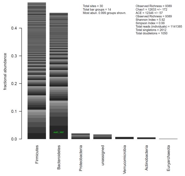
The phyloseq package contains extensions for the default plot methods tailored to the data types present in each phyloseq class. For example, otuSamTax objects can be plotted as a series of stacked bars that represent the relative abundance of phylum-level groups in the combined community, as well as the relative abundance of individual taxa within each phylum (Fig. 2).

Fig. 2.

Example of a default plot method for summarizing an object of class otuSam-Tax. Each phyloseq class has a specialized plot method for summarizing its data. In this case, relative abundance is shown quantitatively in a stacked barplot by phylum. Different taxa within a stack are differentiated by an alternating series of grayscale. The OTU identifier of taxa comprising a large enough fraction of the total community, 5% in this case, is labeled on the corresponding bar segment. Several diversity/richness indices are also shown.

> taxaplot(ex1)

5. Subsetting and filtering

In this particular example, we know that there were two separate Roche-454 sequencing trials included in the QIIME output, but the first sequencing trial (“Run 1”) was of poor quality and should be removed from the dataset. We remove all of the Run 1 samples from ex1 through a simple one-line combination of accessor and replacement methods for the sampleMap slot. On the right-hand side of the assignment operator (<-) we subset the sampleMap, and then assign it to the sampleMap slot of ex1 on the left-hand side. This assignment replaces the originalsampleMap in ex1, and also re-trims the other components of ex1 (e.g. the otuTable) such that only Run 2 samples remain.

> ex1 <- subset_samples(ex1, SeqRun == “R2”)

An alternative approach would be to define a character vector with the sample names of Run 2, and then use the assignment operator: sample.names(ex1)<-. Similarly, we can use species.names()<- assignment to create a new otuSamTaxTree object in which all but the relatively abundant taxa have been trimmed, through a method borrowed from the genefilter package in Bioconductor.²² In this case, we arbitrarily create a filter function that returns TRUE only for the most abundant 30 taxa from a sample, and then apply it to each sample in the otuTable of ex1, with the added parameter that a species must be TRUE in at least four samples (be among the most abundant 30 taxa in four or more samples). Like genefilter, the output of genefilterSample() is a logical vector with the same length as the number of taxa presently in ex1.

> fun1 <- filterfunSample(topk(30))
> wh1 <- genefilterSample(ex1, fun1, A = 4)

The taxa names are then accessed and subsetted based on the value in wh1, and this trimmed vector of taxa names (a total of 52 in this case) is assigned back to our phyloseq object, causing phyloseq’s internal methods to trim the component objects in ex1 to just these taxa. Using a similar approach, we also remove those samples that now contain unacceptably small (< 100, for instance) total numbers of individuals (total reads in this case).

> species.names(ex1) <- species.names(ex1)[wh1]
> sample.names(ex1) <- sample.names(ex1)[sampleSums(ex1) > 100]

6. UniFrac distances

UniFrac is a useful metric to summarize the difference between pairs of ecological communities, and can be used to create a distance matrix for samples in an experiment. An unweighted UniFrac distance matrix only considers the presence/absence of taxa, while weighted UniFrac accounts for the relative abundance of taxa as well as their phylogenetic distance. Presently, only one non-parallelized implementation of the unweighted UniFrac distance is available in R packages (picante::unifrac). In the phyloseq package we provide optionally-parallelized methods for calculating both UniFrac and weighted-UniFrac, as well a few key UniFrac variants, all of which return a sample-wise distance matrix from any phyloseq object that contains both a phylogenetic tree and an otuTable (otuTree and its subclasses).

Here is an example of the weighted UniFrac calculation using a dataset provided in the picante package. We first build an otuTree class object using the phyloseq() constructor, then use the wUniFrac() method to calculate and return the weighted UniFrac distance forall sample pair combinations.

> data(phylocom)
> tree <- phylocom$phylo
> OTU <- phylocom$sample
> ex3 <- phyloseq(otuTable(OTU, speciesAreRows = FALSE), tree)
> wUniFrac(ex3)

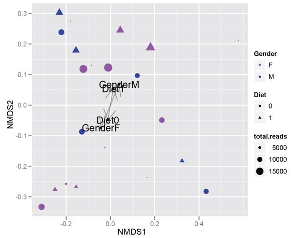
Extending our previous microbiome example, we now calculate the weighted-UniFrac distance matrix for ex1, then perform multi-dimensional scaling on the distance matrix and generate an annotated plot. This can be achieved with the wrapper function wunifracMDS, which also takes advantage of the enhanced plotting facilities provided by the ggplot2 package²⁸ (Fig. 3).

Fig. 3.

NMDS ordination graphic generated by wunifracMDS. The NMDS coordinates are generated by metaMDS(), with the weighted-UniFrac distance matrix as argument, and 2-dimensions specified by default. A separate analysis was done using adonis(), which also did not find a compelling association between the weighted UniFrac distances and the gender (p = 0.29) or diet (p = 0.9) of subjects in the study.

7. Robust multiple-table methods

The NMDS of weighted-UniFrac distances did not reveal any clustering of gut microbiome samples according to a subject’s diet type or gender. However, it may be that these differencesare subtly confined to a subset of species that is not easily detectable with a community-wide summary statistic, like UniFrac. This effect is compounded by the observation that abundance counts as output from high-throughput phylogenetic sequencing have high variabilities,²⁹ leading to a need for robust methods³⁰ that can reveal subtle features of the data.

Many decompositions of inertia³¹ — such as constrained correspondence analysis (cca()), analysis of diversity (adonis()), redundancy analysis (rda()) — use sums of squares. The simplest transformations take the ranked abundances and replace the values by their order statistic. Here we show an example in which we further threshold the ranks so that all the low-abundance taxa at noise-level (where presence/absence of a taxa is as much due to chance as biology) are given the same value.

We can apply this rank threshold transformation to our original data using a special enclosure form of the threshrank() function in phyloseq, and taking the threshold to be 500, for instance. We use a custom method for abundance table transformation in the phyloseq package (transformsamplecounts) that applies one or more transformation functions, in order, to each sample of the otuTable of the first argument. Although it operates only on the otuTable component, transformsamplecounts returns an object with the same class and components as its input.

> ex4 <- transformsamplecounts(ex4, threshrankfun(500))

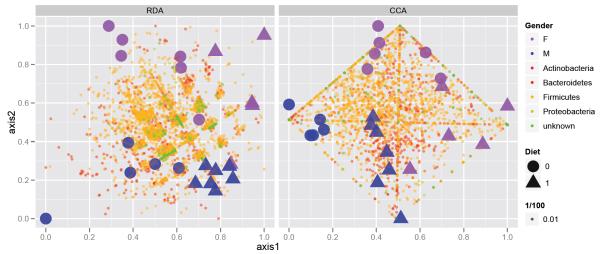
In Fig. 4 we provide the results of a redundancy analysis on the ranked-thresholded abundance table, as well as a constrained correspondence analysis on the original abundance table. These plots were produced using the calcplot() convenience wrapper that — in addition to producing effective graphics with ggplot2 — also provides the opportunity for further graphics manipulation using multiple layers and a mutable graphics description.²⁸ As anticipated, these two methods both appear to effectively cluster the samples by diet and gender, as specified. In addition, these ordination methods indicate which taxa best account for the clustering, which is highly valuable during exploratory analysis.

Fig. 4.

Redundancy analysis and Constrained Correspondence Analysis. (Left) Redundancy analysis applied to a thresholded, ranked-transformed abundance table that had been trimmed such that only the phyla accounting for the top 99% of taxa are included. (Right) Original trimmed abundance table (no transformation nor threshold) subjected to Constrained Correspondence Analysis (CCA), constrained on a subject’s diet and gender.

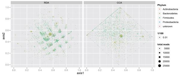
When analyzing a data abundance table with complementary covariates we use generalizations of PCA and Correspondence Analysis that attempt to account for the explanatory variables in the description of the overall variability. Redundancy Analysis (RDA) is a version of PCA with regards to instrumental variables³¹ that tries to predict the multivariate ranked data by the covariates gender and diet. The left side of Fig. 4 shows the graphical output from such an analysis with a biplot representing both the explanatory factors, diet and gender, as well as the OTU distributions as dots. The OTUs actually have a structure formation along the axes of a grid; this is due to the ranking and thresholding of the data. We have magnified this in the left part of Fig. 5 to illustrate the graphical capabilities available through the combination of phyloseq with ggplot2.

Fig. 5.

Enlarged RDA and CCA plots emphasizing the taxa (species) coordinates. Graphics were produced with calcplotrda() or calcplotcca() convenience wrappers in phyloseq, which utilize analysis and graphics tools from the vegan and ggplot2 packages, respectively. Only the phyla accounting for the top 99% of taxa are included.

On the right of Fig. 4 a different type of analysis was used directly on the abundance data, where we performed a constrained correspondence analysis (CCA)³² and projected the output onto the first two constrained coordinates. We have also plotted the covariate groupings and the species. We can see in the magnification of the species plot on the right of Fig. 5 that the grid is replaced by the rhombus of extreme points. These are the OTUs with small abundances which are more strongly weighted in CCA, thus becoming the boundary of the projection region.

8. Functional genes and non-standard phylogenetic markers

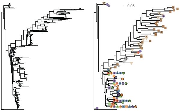
Environmental datasets also utilize novel markers or functional genes for which there is not a large curated database for comparison, nor clustering pipelines carefully tuned to define species-level taxonomic clusters. However, it is common and useful for researchers to calculate a phylogenetic tree from the sequence data, and the source sample from which the individual sequences were derived is generally known. For this situation phyloseq contains a method, tipglom(), that takes as input a phylogenetic tree and sequence-source hash table, and returns a higher-order object, including an otuTable. The tipglom() method uses a default greedy clustering based on a branch-length distance threshold — or an alternative user-provided tree-based method — to agglomerate closely related sequences as one taxa. Each merging step is carried out by a user-accessible method called mergespecies(), which ensures consistency between tree and species abundance tables during each merge. In Fig. 6 we provide an example of an unprocessed tree calculated from more than 400 sequences of the same functional gene, derived from multiple environmental samples. We also show the same tree after processing by the tipglom function (species branch-length cutoff of 0.1), and plotted using a phyloseq method for displaying otuTree objects. In addition to consolidating similar sequences for legibility, this new tree reveals information about particular taxa that appear in multiple samples, as well as portions of the tree that originate from only one sample type.

Fig. 6.

Example of phylogenetic sequence data before and after basic clustering with tipglom() function. (Left) Standard phylogram produced using default plotting function and no OTU clustering. (Right) Annotated phylogram after OTU clustering with tipglom(). Different symbols next to each tip indicate different samples in which the OTU was observed. The number inside each symbol indicates the respective number of individuals of a given OTU were observed in each sample.

9. Conclusions

We describe a new Bioconductor package, phyloseq, for handling, filtering, and analysing high-throughput phylogenetic sequencing data after it has been processed in a sequence clustering pipeline. The phyloseq package provides extensions for leveraging analysis from other ecology-related packages, such as adephylo, vegan, picante, as well as other packages that we have found useful for data of this type. phyloseq also provides useful wrappers for key analysis pipelines that should help to streamline statistical analysis of data from phylogenetic sequencing projects. We hope that this package provides a useful class structure, methods, and methods extensions that will streamline the input of phylogenetic sequencing data, its QC/QA processing and trimming, and especially its analysis and graphical representation by this and other Bioconductor/R packages.

References

- 1.Metzker ML. Nature Reviews Genetics. 2010;11:31. doi: 10.1038/nrg2626. [DOI] [PubMed] [Google Scholar]
- 2.Hamady M, Walker JJ, Harris JK, Gold NJ, Knight R. Nature Methods. 2008;5:235. doi: 10.1038/nmeth.1184. [DOI] [PMC free article] [PubMed] [Google Scholar]
- 3.Pace NR. Science. 1997;276:734. doi: 10.1126/science.276.5313.734. [DOI] [PubMed] [Google Scholar]
- 4.DeSantis TZ, Hugenholtz P, Keller K, Brodie EL, Larsen N, Piceno YM, Phan R, Andersen GL. Nucleic Acids Research. 2006;34:W394. doi: 10.1093/nar/gkl244. [DOI] [PMC free article] [PubMed] [Google Scholar]
- 5.DeSantis TZ, Hugenholtz P, Larsen N, Rojas M, Brodie EL, Keller K, Huber T, Dalevi D, Hu P, Andersen GL. Applied and Environmental Microbiology. 2006;72:5069. doi: 10.1128/AEM.03006-05. [DOI] [PMC free article] [PubMed] [Google Scholar]
- 6.Cole JR, Wang Q, Cardenas E, Fish J, Chai B, Farris RJ, Kulam-Syed-Mohideen AS, McGarrell DM, Marsh T, Garrity GM, Tiedje JM. Nucleic Acids Research. 2009;37:D141. doi: 10.1093/nar/gkn879. [DOI] [PMC free article] [PubMed] [Google Scholar]
- 7.Pruesse E, Quast C, Knittel K, Fuchs BM, Ludwig W, Peplies J, Glöckner FO. Nucleic Acids Research. 2007;35:7188. doi: 10.1093/nar/gkm864. [DOI] [PMC free article] [PubMed] [Google Scholar]
- 8.Li W, Godzik A. Bioinformatics. 2006;22:1658. doi: 10.1093/bioinformatics/btl158. [DOI] [PubMed] [Google Scholar]
- 9.Huang Y, Niu B, Gao Y, Fu L, Li W. Bioinformatics. 2010;26:680. doi: 10.1093/bioinformatics/btq003. [DOI] [PMC free article] [PubMed] [Google Scholar]
- 10.Caporaso JG, Kuczynski J, Stombaugh J, Bittinger K, Bushman FD, Costello EK, Fierer N, Peña AG, Goodrich JK, Gordon JI, Huttley GA, Kelley ST, Knights D, Koenig JE, Ley RE, Lozupone CA, McDonald D, Muegge BD, Pirrung M, Reeder J, Sevinsky JR, Turnbaugh PJ, Walters WA, Widmann J, Yatsunenko T, Zaneveld J, Knight R. Nature Methods. 2010;7:335. doi: 10.1038/nmeth.f.303. [DOI] [PMC free article] [PubMed] [Google Scholar]
- 11.Schloss PD, Westcott SL, Ryabin T, Hall JR, Hartmann M, Hollister EB, Lesniewski RA, Oakley BB, Parks DH, Robinson CJ, Sahl JW, Stres B, Thallinger GG, Van Horn DJ, Weber CF. Applied and Environmental Microbiology. 2009;75:7537. doi: 10.1128/AEM.01541-09. [DOI] [PMC free article] [PubMed] [Google Scholar]
- 12.Giongo A, Crabb DB, Davis-Richardson AG, Chauliac D, Mobberley JM, Gano KA, Mukherjee N, Casella G, Roesch LFW, Walts B, Riva A, King G, Triplett EW. The ISME Journal. 2010;4:852. doi: 10.1038/ismej.2010.16. [DOI] [PMC free article] [PubMed] [Google Scholar]
- 13.Jombart T, Balloux F, Dray S. Bioinformatics. 2010;26:1907. doi: 10.1093/bioinformatics/btq292. [DOI] [PubMed] [Google Scholar]
- 14.Oksanen J, Blanchet FG, Kindt R, Legendre P, O’Hara RB, Simpson GL, Solymos P, Stevens MHH, Wagner H. vegan: Community Ecology Package. (R package version) 2011:1.17–10. [Google Scholar]
- 15.Dray S. Journal of Statistical Software. 2007 [Google Scholar]
- 16.Kembel SW, Cowan PD, Helmus MR, Cornwell WK, Morlon H, Ackerly DD, Blomberg SP, Webb CO. Bioinformatics. 2010;26:1463. doi: 10.1093/bioinformatics/btq166. [DOI] [PubMed] [Google Scholar]
- 17.Paradis E, Claude J, Strimmer K. Bioinformatics. 2004;20:289. doi: 10.1093/bioinformatics/btg412. [DOI] [PubMed] [Google Scholar]
- 18.Schliep KP. Bioinformatics. 2011;27:592. doi: 10.1093/bioinformatics/btq706. [DOI] [PMC free article] [PubMed] [Google Scholar]
- 19.R Hackathon team phylobase: Base package for phylogenetic structures and comparative data. (R package version 0.6.3) 2011 (alphabetically: Ben Bolker, M. Butler, P. Cowan, D. de Vienne, D. Eddelbuettel, M. Holder, T. Jombart, S. Kembel, F. Michonneau, D. Orme, B. O’Meara, E. Paradis, J. Regetz and D. Zwickl) [Google Scholar]
- 20.Beck D, Settles M, Foster JA. Bioinformatics. 2011 doi: 10.1093/bioinformatics/btr196. [DOI] [PMC free article] [PubMed] [Google Scholar]
- 21.R Development Core Team . R: A Language and Environment for Statistical Computing. R Foundation for Statistical Computing; Vienna, Austria: 2011. ISBN 3-900051-07-0. [Google Scholar]
- 22.Gentleman RC, Carey VJ, Bates DM. Genome Biology. 2004;5:R80. doi: 10.1186/gb-2004-5-10-r80. others. [DOI] [PMC free article] [PubMed] [Google Scholar]
- 23.Chambers JM. Software for data analysis. Springer Verlag; 2008. [Google Scholar]
- 24.Yu H. Rmpi: Interface (Wrapper) to MPI (Message-Passing Interface) (R package version 0.5-9) 2010 [Google Scholar]
- 25.Lozupone C, Knight R. Applied and Environmental Microbiology. 2005;71:8228. doi: 10.1128/AEM.71.12.8228-8235.2005. [DOI] [PMC free article] [PubMed] [Google Scholar]
- 26.Lozupone CA, Hamady M, Kelley ST, Knight R. Applied and Environmental Microbiology. 2007;73:1576. doi: 10.1128/AEM.01996-06. [DOI] [PMC free article] [PubMed] [Google Scholar]
- 27.Lozupone C, Hamady M, Knight R. BMC Bioinformatics. 2006;7 doi: 10.1186/1471-2105-7-371. [DOI] [PMC free article] [PubMed] [Google Scholar]
- 28.Wickham H. ggplot2: elegant graphics for data analysis. Springer; New York: 2009. [Google Scholar]
- 29.Zhou J, Wu L, Deng Y, Zhi X, Jiang Y-H, Tu Q, Xie J, van Nostrand JD, He Z, Yang Y. The ISME Journal. 2011 doi: 10.1038/ismej.2011.11. [DOI] [PMC free article] [PubMed] [Google Scholar]
- 30.Holmes S, Alekseyenko A, Timme A, Nelson T, Pasricha PJ, Spormann A. Pacific Symposium on Biocomputing. 2011:142. doi: 10.1142/9789814335058_0016. [DOI] [PMC free article] [PubMed] [Google Scholar]
- 31.Holmes S. Multivariate Analysis: The French Way (Institute of Mathematical Statistics. Beachwood, Ohio; USA: 2008. [Google Scholar]
- 32.Ter Braak CJF. Plant Ecology. 1987;69:69. [Google Scholar]