Models of treatment effects when responses are heterogeneous

Heckman and Vytlacil (1) synthesize and extend a recent body of research in economics and statistics on the identification and estimation of treatment effects when the subjects have heterogeneous responses. This research has demonstrated the importance of distinguishing between several different types of treatment effects and the need to establish firmly the relationship between the different types. Heckman and Vytlacil (H&V) distinguish between four different types: average treatment effects (ATE), effects of the treatment on the treated (TT), local average treatment effects (LATE), and local instrumental variable (LIV) treatment effects. Each is conceptually different, and each has a different set of conditions for identification. The research discussed by H&V represents a genuine advance and clarification of concepts in models of treatment effects.

The framework set up by H&V is heavily influenced by economic and econometric terminology but has major elements that are drawn from statistics as well. The reader may be led to suppose that the concepts and methods are applicable only to observational data and not to randomized clinical trials (RCTs), but this is not the case. All parts of their analysis are equally applicable to both. The application to RCTs is most easily seen by drawing an analogy with intent-to-treat models, as discussed by Angrist et al. (2). Although, in an RCT, the randomization creates a treatment-assignment dummy variable that economists call an “instrument,” similar variables often exist in observational data—natural experiments, quasi-experiments, or, more generally, what economists merely call exogenous identifying variables—and these can satisfy the same conditions as the treatment assignment variable in an RCT, and, hence, the same methods apply.

The major restriction in the models of H&V is the index function restriction, which is the assumption that the propensity to “participate” or “take up” the treatment, when it is offered, can be described by a single function with a single unobservable. H&V note correctly in their conclusions that most of their results can be obtained, in modified form, without an index function restriction, but their analysis in the main makes that assumption. While imposing restrictions, the index function model has great expository and intuitive value in the analysis of treatment effects models.

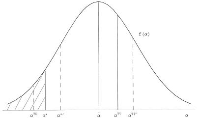
In this commentary, I demonstrate that, with a few additional restrictions, most of the major points discussed by H&V can be given a simple graphical interpretation that has the same virtue of expository usefulness. Denote by α_i the treatment effect for subject i, often called a “random coefficient” in econometric models but equivalent to the heterogeneous treatment response in treatment effect models in statistics. Fig. 1 shows a hypothetical density of α_i in the population, a density assumed to have a mean of ᾱ. This figure appears in Björklund and Moffitt (3), where α_i is given the random coefficient interpretation just referred to. Björklund and Moffitt call α_i the “gain” to the treatment for individual i. Now make the additional restriction that selection takes place strictly on α_i and that, for illustration, selection is positive: subjects with higher values of α_i are more likely to take up the treatment if offered, i.e., more likely to participate.‡ Denote the cutoff value of α_i as α*, above which subjects participate and below which subjects do not.

Figure 1.

Density of treatment gains in a population.

Fig. 1 can be used to illustrate all four estimators. The parameter ᾱ is equivalent to the ATE. The treatment effect on the treated is shown in Fig. 1 as α^TT and is equal to E(α_i|α_i > α*), the mean gain of those who are participants. For future use, Fig. 1 also shows the treatment effect on the untreated, α^TU = E(α_i|α_i < α*), the mean gain that those who are nonparticipants would have if they received the treatment. This quantity is an unobservable. Note that ᾱ = Pα^TT + (1 − P)α^TU, where P = Prob(α_i > α*), by construction.

The LATE estimator is representable in Fig. 1 by a discrete change in α* moving it to α*′, which necessarily shifts α^TT as well, moving it to α^TT′. The LATE estimator equals α^TT − α^TT′ divided by the area under the curve between α* and α*′, which equals the change in the probability of participating. The estimator termed by H&V the LIV is the limit of this change as α*→α*′. This estimator is termed the “marginal” gain by Björklund and Moffitt (3) to emphasize that it is the treatment gain of the marginal subject just on the edge of participating and not participating. A small expansion or contraction of the program will bring these subjects into the program or push them out of it and will lead to a change in the mean gain of participants accordingly. In their empirical example, Björklund and Moffitt analyzed a program that had a positive mean gain for those in the program (positive α^TT) but a negative marginal gain, implying that the program was “too large”—it had been overextended to include subjects who were made worse off by it. Thus the difference between the two can be important.

In general, only α^TT, and changes in that quantity, are identified. This is clear from Fig. 1. Denote the difference between the mean outcome of the subjects of a treatment group that is offered the program and that divides up into participants and nonparticipants in the manner described by Fig. 1, and the mean outcome of a comparison group that is not offered the program at all, as α^UNADJ. Then, it can be shown that α^TT = α^UNADJ/P, where P is the participation rate in the treatment group. Multiple treatment groups with different participation rates can be used with this formula to calculate the LATE estimator and, in the limit, the LIV estimator. Only if P = 1 in one of the treatment groups can ᾱ be identified, as is clear from Fig. 1 (“identification at infinity”).

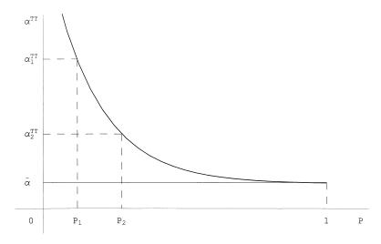
Fig. 2 graphically illustrates this result by showing the relationship between P and α^TT. By the positive and monotonic selection assumed here, the value of α^TT falls and approaches ^-α as P→1. Treatment groups with different values of P form data points along the curve. Two data points are shown in Fig. 2. With two data points, the LATE estimator can be calculated. If the full curve were estimable, what Björklund and Moffitt term the marginal gain and what H&V term the LIV can be calculated as the slope of the curve in Fig. 2.§

Figure 2.

Relationship between participation rate and mean gain of participants.

Fig. 2 suggests what a research agenda on a program should aim to achieve. Estimates from multiple RCTs, observational studies, and other analyses that contain treatment groups with different values of P yield data points on the curve. Nonparametric estimation and related smoothing techniques permit the estimation of the function, at least between the maximum and minimum values of P in the different studies. Extrapolation is required beyond those points.

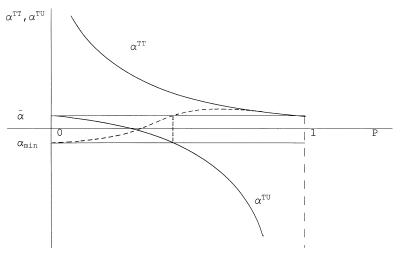
The bounding concepts described in H&V also can be illustrated graphically. Fig. 3 shows both α^TT and α^TU. The latter is an unobservable, as previously noted, and, hence, the α^TU line cannot be estimated. This can be viewed as the reason that ᾱ cannot be estimated as well, for ᾱ = Pα^TT + (1 − P)α^TU is an equation with two estimable quantities, P and α^TT, but two unknowns, ᾱ and α^TU. But if a (say) lower bound α_MIN is established for α^TU, a lower bound on ᾱ can be established as well (note that it is not the bound on the individual y values that matter but only the bound on their difference for the untreated; this is implicit in the formula for the width of the bound). Inserting α_MIN in for α^TU in the weighted average formula for ^-α yields the desired bound for ᾱ. It is illustrated by the dotted line in Fig. 3. Upper bounds could be similarly illustrated.

Figure 3.

Mean treatment gains with an assumed lower bound.

The results in the work by H&V provide a fruitful set of concepts and methods for applications in future research in the social sciences. The different concepts have seen relatively little use to date in applications but should see more in the future.

References

- 1.Heckman J J, Vytlacil E J. Proc Natl Acad Sci USA. 1999;96:4730–4734. doi: 10.1073/pnas.96.8.4730. [DOI] [PMC free article] [PubMed] [Google Scholar]
- 2.Angrist J, Imbens G, Rubin D. J Am Stat Assoc. 1996;91:444–472. [Google Scholar]
- 3.Björklund A, Moffitt R. Rev Econ Stat. 1987;69:42–49. [Google Scholar]