Model-based analysis of multi-shell diffusion MR data for tractography: How to get over fitting problems

Abstract

In this article, we highlight an issue that arises when using multiple b-values in a model-based analysis of diffusion MR data for tractography. The non-mono-exponential decay, commonly observed in experimental data, is shown to induce over-fitting in the distribution of fibre orientations when not considered in the model. Extra fibre orientations perpendicular to the main orientation arise to compensate for the slower apparent signal decay at higher b-values. We propose a simple extension to the ball and stick model based on a continuous Gamma distribution of diffusivities, which significantly improves the fitting and reduces the over-fitting. Using in-vivo experimental data, we show that this model outperforms a simpler, noise floor model, especially at the interfaces between brain tissues, suggesting that partial volume effects are a major cause of the observed non-mono-exponential decay. This model may be helpful for future data acquisition strategies that may attempt to combine multiple shells to improve estimates of fibre orientations in white matter and near the cortex.

Introduction

Acquiring diffusion MRI (dMRI) data with multiple b-values (multi-shell¹) is a requirement of q-space imaging experiments [1]. In tractography applications of dMRI, however, it is common practice to use single shell data with a typical b-value of around 1,000s/mm². Increasing the b-value reduces signal to noise but enhances the angular contrast, which can be beneficial for tractography. Better angular contrast, for a given noise level, can reduce the uncertainty on the estimates of fibre orientations and increase our ability to distinguish fibres that cross at acute angles [2].

Since high b-values give us good contrast and low b-values good signal, it seems natural that we should be combining multiple shells in the same acquisition in order to obtain more accurate local estimates of fibre orientations. An optimal acquisition scheme that finds a good balance between signal and contrast will likely consist of multiple carefully positioned shells. One problem with using multiple b-values is that the diffusion decay curve (signal versus b-value) along any given gradient direction has been shown to follow a non-mono-exponential decay (e.g. [3] and many others). Departure from exponential decay has been observed in both grey and white matter in vivo [4, 5] and ex vivo [6], and appears at around b=1,500s/mm². Interestingly, non-mono-exponential decays have been observed both along and across axonal fibres (e.g. [4]).

The biophysical sources of non-mono-exponential decay in diffusion data are still unclear [7]. Models that account for it include bi-exponential fitting of slow and fast diffusion [8], stretched exponential fitting [9], Kurtosis imaging [10] and statistical models (continuous distributions of diffusion coefficients) [11]. These models are in general more motivated by empirical fitting with parsimony than by biophysical interpretations. Another family of approaches include explicit modelling of restriction effects based on analytic solutions to the diffusion equation [12–18].

Modelling non-mono-exponential diffusion decay can be useful for a better characterisation of diffusion in tissues. It may, for example, provide more specific and interpretable markers of tissue integrity. In the context of tractography, where the focus is mainly on fibre orientation as the most relevant microstructural feature, accounting for non-mono-exponential decay is important for a different reason: avoiding over fitting. Consider the 2D simulation shown in figure 1. The red curves represent signal profiles for 3 different b-values generated using a single-fibre model with multiple diffusion coefficients (the Gamma-distribution model proposed in this article, see the Methods section). In this model, each signal curve contains weighted contributions from infinitely many diffusion coefficients, so when increasing the b-value the lower diffusion coefficients contribute more to the signal, leading to an apparent slower decay. Fitting a single fibre model with a single diffusion coefficient [19] to this data, the decay curves fail to capture the shape of the simulated signal. In particular, the signal predictions along the fibre (the direction of lowest signal) show faster decays for the single diffusivity model. Adding extra fibres to this mono-exponential model captures the slower decay at higher b-values. Intuitively, restricted diffusion across the extra fibres compensates for the faster decay along the main fibre in the mono-exponential model. This over-fitting can have catastrophic consequences in the context of tractography. The extra orientation parameters, whilst important for fitting the data (and hence may not be excluded by model selection), can lead to many false positive connections from tractography.

Figure 1.

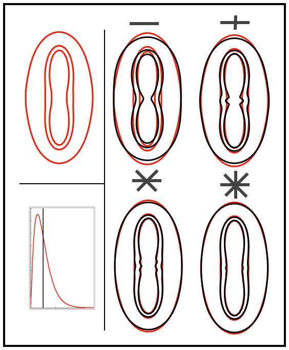
Illustration of the over-fitting using two-dimensional simulations. Top left: signal profile for a single fibre model using Gamma distributed diffusivities and 3 b-values = (1,2 and 3)×10³ s/mm². Right panel: black lines are maximum likelihood fits of the mono-exponential model with increasing number of crossing fibres (1,2,3 and 4). Notice how increasing the number of fibres artificially moulds the predictions to the simulated data, even though the data was generated using a single fibre. Bottom left: distribution of diffusivities for the red (Gamma) and black (dirac) signals.

In this article we propose a simple solution to this problem. We introduce a model that allows for a continuous distribution of diffusion coefficients using a Gamma distribution. The model only has one extra parameter compared to the mono-exponential model. This is very useful in tractography applications that use high angular resolution diffusion imaging (HARDI). Due to scanning time constraints, many gradient directions are acquired, but only a few shells may be afforded. In contrast, experiments that use many b-values along two or three gradient directions can afford to use more complex (and arguably more adequate) decay models. The use of a Gamma distribution of diffusivities leads to a very simple signal equation. Apart from parsimony and simplicity, another benefit of this model is that by re-interpreting the parameters of the Gamma distribution in terms of mean and variance of diffusivities, it is possible to use a shrinkage prior on the variance parameter [2], which is equivalent to getting back to the simpler mono-exponential model in the case where the data do not support the more complex model (e.g. single shell data or multi-shell but low b-value data).

It is important to stress here that the over-fitting problem introduced above and in figure 1 is an issue for model-based approaches to tractography. More specifically, models that explicitly represent fibre orientations require an assumption as to the form of the signal decay as a function of the fibre orientation. If this fibre response kernel is assumed to decay mono-exponentially, we get spurious orientations and over-fitting to multi-shell data. In contrast, model-free approaches may have similar or different issues related to multi-shell data, depending on the assumptions that they make and on the goals that they are trying to achieve. In this paper, we will focus on a model-based approach (the ball and stick model [19]), but we will come back to this important point in the discussion.

Using in-vivo experimental data, we show that the Gamma-distribution model dramatically decreases over-fitting. In particular, voxels that are at interfaces between brain tissues show the most improved fits. This suggests that the apparent departure from mono-exponential decay, at least in our data, is mainly driven by partial volume effects. However, another possible explanation for an apparent non-mono-exponential decay can be that the signal reaches the noise floor [20]. Our attempt to account for this possibility is twofold. Firstly, a Rician noise model is used throughout all the experiments instead of the Gaussian model. Secondly, we compare our Gamma distribution model to a simpler noise floor model that has the same number of extra parameters. We show that the Gamma distribution model mostly outperforms the noise floor model, particularly in voxels at interfaces between tissue types, and even more so when we include a smaller shell (b=300 s/mm², 20 directions). As the smaller shell contains more cerebro-spinal fluid (CSF) contamination, our results suggest that partial volume effects contribute significantly to the departure from mono-exponential decay.

Methods

The model(s)

The following is an extension of the ball and stick model [19] to multiple diffusivities.

The ball and stick signal attenuation A_i has the following generic form:

$$A_i=\frac{s_i}{s_0}=(1-{\sum }_k{f}_k)exp(-b_{i}d)+{\sum }_k{f}_{k}exp(-b_{i}d{(g_i^T{x}_k)}^2)$$ [1]

In the above equation, S₀ is the signal with no diffusion weighting, S_i the signal with a diffusion gradient applied along the unit vector g_i with b-value b_i. The {f_k} are volume fractions for the different fibre compartments. Each compartment is modelled using a degenerate stick-like tensor (i.e. rank=l) oriented along {x_k}. Isotropic diffusion is modelled using the same diffusion coefficient as non-isotropic diffusion and is represented by a separate compartment that attempts to explain any signal that is not captured by the sticks. Notice that all the diffusion-related decays in this model have the general form exp(−bdg) where g is equal to 1 for the isotropic compartment and to cos(θ)² for the anisotropic compartment, where θ is the angle between diffusion gradient and fibre orientation. We refer to this model as mono-exponential because it has a single diffusion coefficient; although strictly speaking it is a sum of exponentials along any given gradient orientation. This model is only exactly mono-exponential along the major fibre orientation (assuming a single anisotropic compartment). If we consider now a continuous Gamma distribution of diffusivities, the above model can be re-written:

$$\check{A}={\int }_0^{\infty }Ap(d)\text{d}d$$ [2]

Where p(d)~Γ(α,β) is a Gamma distribution with shape parameter α and scale 1/β. The above integral can be evaluated analytically for the generic decay term of the form {exp(−bdg)}:

$${\int }_0^{\infty }exp(-\mathit{bdg})p(d)\text{d}d={\int }_0^{\infty }exp(-\mathit{bdg})\frac{{\beta }^{\alpha }}{\mathrm{\Gamma }(\alpha )}{d}^{\alpha -1}exp(-d/\beta )\text{d}d={\left(\frac{\beta }{\beta +bg}\right)}^{\alpha }$$ [3]

Plugging this final result into equation [1], and replacing {g} by the appropriate quantity in each compartment, we get the following formula:

$$\frac{s_i}{s_0}=(1-{\sum }_k{f}_k){\left(\frac{\beta }{\beta +b_i}\right)}^{\alpha }+{\sum }_k{f}_k{\left(\frac{\beta }{\beta +b_i{(g_i^T{x}_k)}^2}\right)}^{\alpha }$$ [4]

Note that fitting a continuous distribution of diffusivities that is not bounded between 0 and infinity may seem artificial. However, the effective contributions of higher diffusivities die out exponentially due to the use of the Gamma function.

Now, in the results section we are going to compare this statistical model to a model that includes a noise floor compartment. This is similar in spirit to the maximum-likelihood approach introduced for the diffusion tensor model in [20]. We model the noise floor using a scalar parameter that accounts for the fraction of the signal that does not decay with diffusion weighting. This model has been suggested previously to account for physical compartments where water is trapped so the diffusion coefficient is effectively zero [21]. Here we do not attempt to make the distinction between this possibility and an actual noise floor, as both capture the same feature in the data. The model writes:

$$\check{A}=f_0+(1-f_0)A$$ [5]

Where A is the mono-exponential signal and f₀ is a scalar between 0 and 1. Notice here that f₀ does not depend on the b-value or the gradient direction whereas A does.

Comments on the model and its inversion

The above model, which has already been suggested in the context of isotropic diffusion by Yablonski et al [22], uses a continuous Gamma distribution. An alternative statistical model has also been suggested by the same group [11], this time using a truncated Gaussian distribution (as diffusivities cannot be negative). We have chosen the Gamma function because of its simplicity; the integral is analytic and the final signal expression fast to evaluate. The parameters α and β of the Gamma distribution are related to the mean and variance of the distribution as follows:

$$\begin{array}{l}\text{Mean}=\alpha /\beta \\ \text{Variance}=\alpha /{\beta }^2\end{array}$$

When the variance parameter is equal to zero, the model simplifies to the original ball and stick with a single scalar diffusion coefficient. In our implementation, we use Bayesian Monte Carlo sampling [19] to estimate posterior distributions on all model parameters. We use a shrinkage prior (automated relevance determination – A.R.D.) on the standard deviation of diffusivities (sqrt{α/β²}) [23], which is conceptually similar to the prior on fibre compartments that we have used previously [2]. The latter allows us to select the number of fibre compartments that is supported by the data; the former allows us to determine whether a single diffusion coefficient is sufficient to fit the data, on a voxel by voxel basis. In practice, during the sampling, we resort to the mono-exponential model whenever sqrt{α/β²} is smaller than 10⁻⁵ mm²/s. We found using simulations that below this value, the two models give the same signal decay to within a relative error of 10⁻⁷ or lower. For all other parameters in the model, we use the same priors as described in previous publications [2, 19]. We also use the same ARD prior on the f₀ parameter in the noise floor model. All model parameters are initialised with non-linear maximization of the Likelihood function using Levenberg-Marquardt optimisation with Gauss-Newton Hessian approximation [24]. A Rician noise distribution was assumed with an unknown variance parameter that was also fitted to the data using the same sampling technique.

Results

Data and pre-processing

Single-shot echo planar diffusion-weighted MRI data were acquired from a single healthy volunteer on a Siemens 3T Verio using a 12-channel head-coil. Sequence parameters were as follows: Twice re-focused Pulsed Gradient Spin-Echo sequence [25], 55 contiguous axial slices, isotropic (2×2×2mm) resolution, TR/TE=9000/115ms. Three sets of 60 diffusion weighted volumes were acquired with 3 different b-values (1/2/3)×10³ s/mm² using the same gradient orientation table (isotropically distributed on the sphere). Additionally, 14 non-diffusion weighted (b=0) volumes were acquired: 11 at the beginning of the experiment, and one before each set of 60 diffusion weighted volumes. A Gradient-echo-based field map was also acquired using the following parameters: (3×3×3mm) voxels, TR=548ms, TE1=5.19ms, TE2=7.65ms, Flip Angle=60deg.

The diffusion data were pre-processed using tools from FSL 4.1 [26, 27]. No eddy-current correction was applied. This is because we noticed that the high b-value images were better aligned prior to the correction, given the high tissue contrast compared to the lower b-values. Examining the data visually, it seemed that the eddy-currents were compensated for by the twice-refocused strategy. Field map-based EPI distortion correction was applied using FUGUE [28]. Head motion was estimated using a FLIRT affine transformation with 6 degrees of freedom (translations and rotations) [29]. Each diffusion-weighted volume was first registered to the nearest b0, then to the very first b0. The full transformation (including EPI distortion unwarping, and the two rigid-body transformations to the b0s) was then applied to every volume independently. The quality of these registration steps was visually assessed. The gradient orientations were rotated to account for the rigid component of these transformations [30].

We used Bedpostx (part of the FDT tool in FSL) to fit the ball and stick model on a voxel by voxel basis. Bedpostx generates samples from the posterior distribution on all model parameters using the Metropolis Hastings sampling algorithm as described in [19]. We fitted three fibre compartments per voxel. Additionally, we fitted the Gamma distribution model with a shrinkage prior on the standard deviation of diffusivities (sqrt{α/β²}) using the same number of fibre compartments, as well as the noise floor model with a shrinkage prior on f₀. compartment where the prior was uniform between 0 and 1. In all the results below, we consider the mean posterior distribution for our parameter estimates.

Gamma model

A comparison between the standard ball and stick model and our extension using a Gamma distribution of diffusivities shows a significant reduction in over-fitting. Figure 2 illustrates this with maps of the mean posterior distribution on the volume fractions. Of particular interest are the volume fractions for the second and third fibre within every voxel. We can see that for the mono-exponential model, the shrinkage prior fails to supress the extra compartments. This is especially true near the cortex, but happens even in regions where we expect a single fibre to be sufficient (e.g. in the medial sections of the corpus callosum). The third fibre (in blue) is mainly present at the interface between grey and white matter (or grey matter and CSF), and may reflect partial volume effects. By contrast, the Gamma distribution model successfully selects the appropriate number of fibres per voxel. Quantitatively, the proportion of brain voxels with a volume fraction above 0.05 was equal to 50% (resp. 26%) for the second fibre, and to 21% (resp. 5%) for the third fibre when using the mono-exponential (resp. Gamma) model. In other words, only half of the voxels identified as containing (at least) two crossing fibres with the ball and stick model were considered so in the Gamma model. This proportion dropped to a quarter for three-way crossings.

Figure 2.

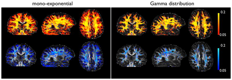
Maps of the mean posterior volume fractions for the second (yellow-red) and third (blue) fibre compartments. All maps are thresholded at 0.05. The mono-exponential model fits a second fibre everywhere except in the ventricles and parts of the corpus callosum. A third fibre is fitted at the interface between CSF and brain tissue. The aternative Gamma distribution model only supports crossing fibres in white matter areas.

Next we examined the spatial histograms of the parameters from the anisotropic compartments (volume fractions and orientations). The first row in figure 3 shows histograms of the volume fractions. From that figure, we can see that the Gamma and noise floor models have similar distributions. We can also see that the second and third compartments have higher volume fractions for the mono-exponential model, particularly in the range around a fraction of ~0.1, indicating over-fitting. The second row in figure 3 represents histograms of the dispersion of the fibre orientation around its mean. The dispersion is a scalar value that represents the uncertainty on the fibre orientation encoded in the posterior distribution. It is defined as 1-Λ, where Λ is the highest eigenvalue of the average dyadic tensor of all posterior sample orientations. This leads to a scalar between 0 (low dispersion/uncertainty) and 1 (high dispersion/uncertainty). The mono-exponential model clearly shows much lower dispersions on the second and third fibre compartments. This is consistent with the over-fitting problem, and indicates that the shrinkage prior has not been able to discard those extra-compartments, as they helped fit to the high-b-value data. Note that the bump for these two fibre populations nearer higher dispersion levels corresponds to voxels where these two compartments have been suppressed by the ARD criterion.

Figure 3.

Histograms (across voxels) of the volume fractions (top) and fibre orientation dispersion (bottom) for the three fibre compartments. The dispersion is calculated from posterior sample orientations. Higher values mean higher uncertainty (see main text). The three models give similar histograms for the first fibre. For the second and third fibre, we can see that: (1) the Gamma and noise floor models give similar histograms; and (2) the mono model has lower uncertainty and a peak of volume fractions that corresponds to the voxels with overfitting.

Comparison to the noise floor model

In order to compare the Gamma model with the (conceptually) simpler noise floor model, we calculated a map of relative sum of squared errors (SSE) in model fit. This map, shown in figure 4, displays the following quantity: (SSE_f0 − SSE_gamma)/(SSE_f0+SSE_gamma), i.e. the relative difference between the two model fits. In voxels with a negative (resp. positive) value, the noise floor (resp. Gamma) model has lower relative SSE between the data and the model prediction. Bearing in mind that both models have the same number of parameters, this gives us a balanced estimate of relative goodness of fit. We can see that the noise floor model performs better in voxels on the edges of the brain, while the Gamma model has lower relative error in voxels at interfaces between tissue types, possibly supporting partial volume effects (see also Figure 8 and related comments in the discussion). Figure 5 shows spatial maps of the extra parameters from the Gamma model (standard deviation of diffusivities) and the noise floor model (f₀). The maps show that these parameters are “needed” in the same brain areas.

Figure 4.

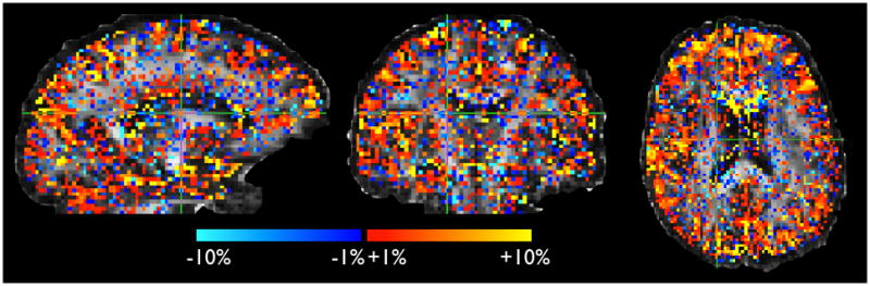
Relative difference in sum-of-squared errors between data and predictions from Gamma and noise floor models. Error is smaller for the Gamma models in the red voxels, and smaller for the noise floor model in the blue voxels. This map is thresholded at 1%. We can see that the Gamma model gives better fits on the interface voxels between grey and white matter. Note that the two models have the same number of parameters.

Figure 8.

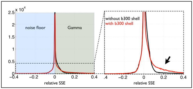
Histograms of relative difference in sum-of-squared error (SSE) between noise floor model and Gamma distribution model. The figure shows the same histogram from fitting the models to data with (red) and without (black) a smaller shell (b=300 s/mm², 20 directions). Negative (resp. positive) SSEs correspond to areas where the noise floor model performs better (resp. worse) than the Gamma model. It is clear that adding a small shell improves the fit where the Gamma model outperforms the noise floor model, suggesting a better modelling of partial voluming with CSF. The left hand-side of the histogram remains unchanged.

Figure 5.

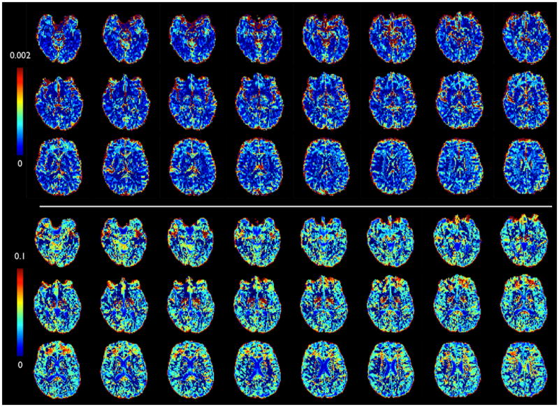
Maps of the extra parameters. Top: Standard deviation of the Gamma distribution in diffusivities (sqrt(α)/β in mm²/s); Bottom: noise floor parameter (f₀).

An informative, but not often used, way to look at the data is to plot the signal as a function of the squared dot product between the gradient and fibre orientations. Figure 6 shows these plots for an example voxel in the genu of the corpus callosum (medial section). The data are plotted on a logarithmic scale, which means that a mono-exponential model with a single fibre predicts a near-linear relationship², which can be contrasted with the nonlinear behaviour of the two other models. Adding two extra fibre compartments produces clear over-fitting for the standard model, and a slight over-fitting for the noise floor model. This effect relates to the intuitive explanation that we have given in figure 1. Two extra crossing-fibres are utilised by the mono-exponential model to mould the signal by reducing the attenuation along the main fibre. The continuous Gamma model is able to produce a better fit without extra fibres by correctly accounting for the non-mono-exponential decay. Recall that a shrinkage prior was used on the second and third fibre for all three models. Unlike the mono-exponential model, the Gamma model produces a smooth curve, consistent with it only fitting a single fibre due to the shrinkage prior.

Figure 6.

Data and model fits from a voxel in the medial section of the genu of the corpus callosum. Top: 1 fibre fit, bottom: 3 fibres fit. The noise level is defined as the average data from a group of voxels outside the brain. Log-data is plotted as a function of the angle between the main fibre orientation predicted by each model and the gradient orientations for the three shells. We can see clear overfitting in the mono model, and a little overfitting in the noise floor model.

Do we benefit from multi-shell data?

In the introduction, we suggested that combining multiple shells may allow us to benefit from both the high contrast of high-b shells and high SNR or the low-b shells. While a full study of optimal schemes for choosing the number and position of shells is out of the scope of this paper, we present a simple proof-of-concept comparison to examine the benefit of multiple shells in our experimental data. We compared 60 directions multi-shell data (i.e. 3×20 directions) to 60 directions single shell data using the following bootstrap procedure. From our complete set of 3×60 directions multi-shell data set, we randomly selected 20 non-parallel orientations from each shell, such that the total 60 orientations cover the same gradient set as each single shell data. We repeated this bootstrap process 100 times to produce histograms of volume fractions and orientation dispersions after fitting a 3-fibres ball and stick model. We used the Gamma model for the 3×20 multi-shell data and the mono-exponential model for the single shell data. Figure 7 shows the results for 2 voxels where we expect a single fibre orientation (genu of the corpus callosum) and a 3-way fibre crossing (centrum semiovale) respectively. The figure shows that in the corpus callosum voxel, all data sets provide the same results, fitting the correct number of fibres and having a similar uncertainty on the orientation. However, in the centrum semiovale, the single shell data fail to recover crossing fibres, favouring a simpler model with a weak single fibre combined with an isotropic diffusion profile. This is not surprising, as in 3-way crossing voxels, the single-shell signal profile is quasi-spherical, favouring a large contribution from the isotropic pool. The multi-shell data, on the other hand, was able to yield lower uncertainty and up to 2 (resp. 3) fibre fits in 86% (resp. 42%) of the cases (threshold on volume fraction=0.05). A whole brain analysis using one of the 20×3 multi-shell schemes showed that a 3-way crossing was detected in 0.45% of the voxels for the multi-shell data, compared to 0.04, 0.14 and 0.15% in the b1000, 2000 and 3000 single-shell data respectively. Note that the full data set contained 5% of 3-way crossings. The voxels detected from the reduced data sets were a subset of these 5%.

Figure 7.

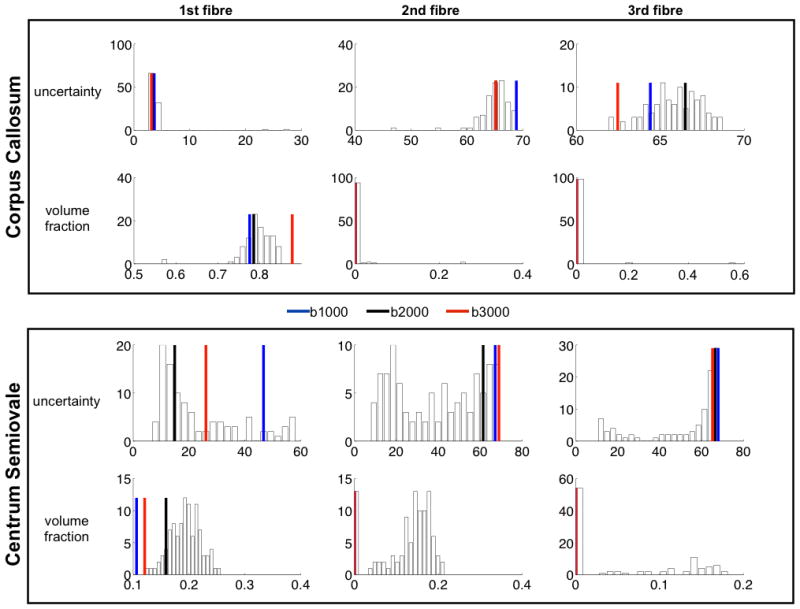
Performance of 60 directions single versus multi shell. The histograms show distributions across 100 bootstrap multi-shell data sets with 3×20 directions (see main text). The colored vertical bars are parameter estimates for the b1000 (blue), b2000 (black) and b3000 (red) single shell data. The Gamma model was fitted to the multi-shell data, and the equivalent results in the corpus callosum voxel. However only in the case of the multi-shell data were we able to fit a 3-way crossing (indicated by lower uncertainty and higher volume fraction). Uncertainty is shown in degrees.

Discussion

In this paper we suggested a simple strategy for using multi-shell data in the context of tractography. The benefits of multi-shell data for estimating fibre orientations are still unclear; the balance between gain in contrast and loss in signal needs to be investigated in a dedicated study. Here we argue that when multi-shell data are used for tractography, they require extra care, as standard models of fibre orientation fail and tend to over-fit by creating artificial fibre crossings. It should be noted, however, that all the discussion so far has been centred on the ball and stick model. Many alternative strategies to map diffusion data onto axonal orientation exist; it is therefore appropriate to discuss here multi-shell data in the context of these other strategies.

Most methods for mapping fibre orientations from diffusion data attempt to reconstruct an orientation distribution function (ODF), a function on the sphere whose peaks align with axon orientation(s). Multiple peaks are generally thought to represent multiple potential axon orientations. The most common ODFs of interest are the diffusion ODF (dODF) and the fibre ODF (fODF). The former represents the probability of diffusion along any given direction, and the latter the probability that fibres are aligned along any given axis. In the case of the ball and stick model, the fODF is explicitly modelled as a weighted sum of sticks (rank-1 tensors). An alternative approach is to estimate the fODF directly from the data using deconvolution [31–33]. However, most of the deconvolution approaches, whilst not assuming a specific form for the fODF, need to incorporate a model for the single fibre response function [31, 34–36] (i.e. a model for the signal profile when the fODF is a stick). Therefore, the same argument on accounting for non-mono-exponential decay applies: in order to cope with multi-shell data, the fibre response function needs to be able to model non-mono-exponential decay. A slightly different approach is followed in Tournier et al. [33], where the fibre response function is obtained from the most anisotropic voxels in the data and described “non-parametrically”, using rotational/spherical harmonics. In this approach, the harmonics are polynomial functions with no radial components; i.e. the method assumes single-shell data.

Methods that reconstruct the diffusion rather than the fibre ODF also exist. The diffusion spectrum imaging (DSI) technique attempts to recover the full diffusion propagator [37] from q-space data and then obtain the dODF by radial integration of the propagator. Since DSI is based on a Fourier inversion of q-space data, multiple b-values are a requirement of the method (Cartesian sampling, as opposed to concentric shells, being more appropriate in this case). While no explicit model for multi-exponential decay needs to be assumed in DSI, it is still important to account for the noise floor issue. In fact it is an even bigger problem in DSI because of the high b-values required, and the need for acceleration to reduce imaging time (which also may affect the noise distribution). Different approaches have been proposed to filter noisy signal intensities; for instance, a Hanning filter is employed in [37], and statistical thresholding using a Gamma distribution of the intensities is proposed in [38]. All these approaches suppress signals that are close to the noise floor, effectively reducing the angular resolution of the resolved propagator.

Another popular method for estimating the dODF is the Qball imaging approach [39], which also attempts at reconstructing the dODF directly from the data with no assumption as to its form (model-free). The original Qball formalism is based on a spherical integral of the signal within a shell. Therefore, in principle, it is designed for single-shell data. An extension of Qball has recently been proposed by Aganj et al. that integrates over multiple shells [40]. This method makes a multi-exponential assumption on the signal decay with b-value. Aganj et al. showed results for a bi-exponential fitting and found that when a mono-exponential assumption is used instead for multi-shell acquisitions, the dODFs are less sharp and, depending on the b-values used in the acquisition, their maxima may not necessarily coincide with the true fibre orientations. Notice that this is not the same effect as in our model-based approach, whereby non-mono-exponential decay produces spurious orientations.

Apart from fODF and dODF-based techniques, other variants have been introduced to estimate fibre orientations from dMRI data. A different deconvolution approach has been introduced by Jansons and Alexander [41] that aims to estimate the angular structure of the diffusion propagator that persists across radial contours (PAS-MRI). Although, to our knowledge, it has not yet been shown in the literature, we anticipate that the deconvolution kernel of PAS should be able to capture multi-exponential behaviour, given that the appropriate filtering parameter is chosen. Similar to PAS, the diffusion orientation transform (DOT) is an ODF variant [42] that transforms the signal to probability profiles of diffusion displacements. Although DOT was initially designed under a mono-exponential model assumption, it can be extended to a multi-exponential version. Using the mono-exponential assumption in multi-shell data, the profiles will appear broader [42], reducing the angular resolution of the method. Furthermore, this assumption may lead to spurious peaks, if high b-values are utilised [43].

Another point of discussion is our choice of the statistical model (Gamma distribution) that captures the non-mono-exponential decay. This is somewhat independent of the choice of the model for capturing orientation per-se. Alternatives to our approach include, as we have mentioned in the introduction, the popular bi-exponential model, Kurtosis imaging (second order Taylor expansion of the log-data as a function of b-values), the stretched exponential model, and the more biophysical models (e.g. restricted diffusion in cylinders). We have chosen the simplest possible extension to our previous model, i.e. by adding one single scalar parameter. The bi-exponential model, in contrast, has two more parameters than the mono-exponential. It is likely that this model may give better fits to data acquired using multiple b-values (e.g. more than 10) along any given direction. In fact, it has been shown that when several orders of magnitude in b-values are used, even the bi-exponential model fails to fit the data accurately [16]. However, tractography applications typically require dense coverage of the sphere with gradient orientations. The number of shells that can be acquired is therefore limited by scan time. We think that in such situations, it is crucial to have fewer parameters for capturing the feature that is implied by the few extra shells.

It is interesting to see that an even simpler model, that of a noise floor, was able to fit the data (although see figure 4). This point is important and needs further investigation: are we measuring truly non-exponential decay, or are we simply not modelling the effect of noise correctly? Answering this question will require further improvements in the reconstruction of multi-channel acquisitions, as well as a better noise model. In this paper, we have used the adaptive-combined reconstruction method [44], as opposed to the more standard sum-of-squares method, and we fitted the data using a Rician noise assumption. Yet, it was not sufficient to overcome the over-fitting issue. We are currently investigating other reconstruction strategies that may improve on this issue. We would also like to point out that the noise-floor problem is not only an issue for multi-shell data; it can affect even single-shell data, especially at high b-values. For example, Jones et al [20] has already shown that noise floor can give biased estimates of the apparent diffusion coefficient and fractional anisotropy in diffusion tensor imaging.

Comparing the fits from the noise floor and the statistical models, we have found that the Gamma model has smaller errors mainly at interfaces between tissue types. This suggests that the statistical model is better at modelling partial volume effects. To test this claim, we acquired an extra (smaller) shell at b=300 s/mm² (25 evenly distributed directions). At such diffusion weighting, the signal still contains a significant contribution from the cerebrospinal fluid (CSF); thus, combining this data with the higher shells exacerbates any partial volume effects with CSF. Figure 8 shows histograms of relative SSEs differences between the two models. We can clearly see that when adding the extra shell, the statistical model performs even better (compared to the noise floor model), suggesting that the voxels where the statistical model is favoured do indeed contain partial volume effects.

This last observation may seem at odds with our Gamma model. CSF has an isotropic contribution to the signal, yet we found that it may relate to the apparent non-mono-exponential behaviour. Why then use a Gamma model for both iso- and anisotropic pools? Perhaps the Gamma distribution model may be more appropriate for the isotropic compartment than for the anisotropic (restricted) compartment. We tested this hypothesis by comparing the Gamma model on both compartments to a Gamma model on the isotropic compartment and mono-exponential model on the anisotropic compartments. We kept the same number of parameters by constraining the mean diffusivity of the isotropic compartment to equal the diffusion coefficient of the anisotropic pool. Interestingly, we found no difference in the model fits between these two models. They performed equally well, and outperformed the noise floor model in the same way, including with the b=300 shell. We do not intend to make biophysical claims on the basis of only 3 shell data, given the long history of experimental results that exhaustively sample b-space. Our purpose in this paper is to fit fibre orientations without over-fitting in orientation-space. As these two models have the same performance in this respect, we do not favour either of them.

Finally, let us come back to the question of whether multi-shell data can be a better solution for tractography. It will certainly be beneficial in the future to investigate the optimal positioning of the different shells in multi-b-values acquisitions. This is not a trivial question though. For example, it is likely that higher b-value shells may benefit from more angular coverage than lower shells. Also, it may be more optimal to acquire different shells using different (optimised) echo times, to maximise the SNR of each acquisition (T₂ decay could be accounted for by acquiring separate b=0 images for each shell). In our data, we found that multi-shell outperformed single-shell data when comparing 60 directions data sets. However, this may not necessarily be the case had we compared data with a denser coverage of the sphere, different sets of b-values or different SNRs. Ultimately, a simulation study is needed to quantify the effects of these parameters and their interactions, and derive a strategy for designing shell positioning.

References

- 1.Callaghan PT. NMR imaging, NMR diffraction and applications of pulsed gradient spin echoes in porous media. Magn Reson Imaging. 1996;14:701–709. doi: 10.1016/s0730-725x(96)00152-x. [DOI] [PubMed] [Google Scholar]
- 2.Behrens TE, Berg HJ, Jbabdi S, Rushworth MF, Woolrich MW. Probabilistic diffusion tractography with multiple fibre orientations: What can we gain? Neuroimage. 2007;34:144–155. doi: 10.1016/j.neuroimage.2006.09.018. [DOI] [PMC free article] [PubMed] [Google Scholar]
- 3.Niendorf T, Dijkhuizen RM, Norris DG, van Lookeren Campagne M, Nicolay K. Biexponential diffusion attenuation in various states of brain tissue: implications for diffusion-weighted imaging. Magn Reson Med. 1996;36:847–857. doi: 10.1002/mrm.1910360607. [DOI] [PubMed] [Google Scholar]
- 4.Clark CA, Le Bihan D. Water diffusion compartmentation and anisotropy at high b values in the human brain. Magn Reson Med. 2000;44:852–859. doi: 10.1002/1522-2594(200012)44:6<852::aid-mrm5>3.0.co;2-a. [DOI] [PubMed] [Google Scholar]
- 5.Mulkern RV, Gudbjartsson H, Westin CF, Zengingonul HP, Gartner W, Guttmann CR, Robertson RL, Kyriakos W, Schwartz R, Holtzman D, Jolesz FA, Maier SE. Multi-component apparent diffusion coefficients in human brain. NMR Biomed. 1999;12:51–62. doi: 10.1002/(sici)1099-1492(199902)12:1<51::aid-nbm546>3.0.co;2-e. [DOI] [PubMed] [Google Scholar]
- 6.Beaulieu C, Allen PS. Determinants of anisotropic water diffusion in nerves. Magn Reson Med. 1994;31:394–400. doi: 10.1002/mrm.1910310408. [DOI] [PubMed] [Google Scholar]
- 7.Mulkern RV, Haker SJ, Maier SE. On high b diffusion imaging in the human brain: ruminations and experimental insights. Magn Reson Imaging. 2009;27:1151–1162. doi: 10.1016/j.mri.2009.05.003. [DOI] [PMC free article] [PubMed] [Google Scholar]
- 8.Clark CA, Hedehus M, Moseley ME. In vivo mapping of the fast and slow diffusion tensors in human brain. Magn Reson Med. 2002;47:623–628. doi: 10.1002/mrm.10118. [DOI] [PubMed] [Google Scholar]
- 9.Bennett KM, Schmainda KM, Bennett RT, Rowe DB, Lu H, Hyde JS. Characterization of continuously distributed cortical water diffusion rates with a stretched-exponential model. Magn Reson Med. 2003;50:727–734. doi: 10.1002/mrm.10581. [DOI] [PubMed] [Google Scholar]
- 10.Jensen JH, Helpern JA, Ramani A, Lu H, Kaczynski K. Diffusional kurtosis imaging: the quantification of non-gaussian water diffusion by means of magnetic resonance imaging. Magn Reson Med. 2005;53:1432–1440. doi: 10.1002/mrm.20508. [DOI] [PubMed] [Google Scholar]
- 11.Yablonskiy DA, Bretthorst GL, Ackerman JJ. Statistical model for diffusion attenuated MR signal. Magn Reson Med. 2003;50:664–669. doi: 10.1002/mrm.10578. [DOI] [PMC free article] [PubMed] [Google Scholar]
- 12.Assaf Y, Blumenfeld-Katzir T, Yovel Y, Basser PJ. AxCaliber: a method for measuring axon diameter distribution from diffusion MRI. Magn Reson Med. 2008;59:1347–1354. doi: 10.1002/mrm.21577. [DOI] [PMC free article] [PubMed] [Google Scholar]
- 13.Jespersen SN, Kroenke CD, Ostergaard L, Ackerman JJH, Yablonskiy DA. Modeling dendrite density from magnetic resonance diffusion measurements. Neuroimage. 2007;34:1473–1486. doi: 10.1016/j.neuroimage.2006.10.037. [DOI] [PubMed] [Google Scholar]
- 14.Neuman CH. Spin echo of spins diffusing in a bounded medium. The Journal of Chemical Physics. 1974;60:4508–4511. [Google Scholar]
- 15.Sen PN, Basser PJ. A model for diffusion in white matter in the brain. Biophys J. 2005;89:2927–2938. doi: 10.1529/biophysj.105.063016. [DOI] [PMC free article] [PubMed] [Google Scholar]
- 16.Stanisz GJ, Szafer A, Wright GA, Henkelman RM. An analytical model of restricted diffusion in bovine optic nerve. Magn Reson Med. 1997;37:103–111. doi: 10.1002/mrm.1910370115. [DOI] [PubMed] [Google Scholar]
- 17.Szafer A, Zhong J, Gore JC. Theoretical model for water diffusion in tissues. Magn Reson Med. 1995;33:697–712. doi: 10.1002/mrm.1910330516. [DOI] [PubMed] [Google Scholar]
- 18.Tanner JE, Stejskal EO. Restricted Self-Diffusion of Protons in Colloidal Systems by the Pulsed-Gradient, Spin-Echo Method. The Journal of Chemical Physics. 1968;49:1768–1777. [Google Scholar]
- 19.Behrens TE, Woolrich MW, Jenkinson M, Johansen-Berg H, Nunes RG, Clare S, Matthews PM, Brady JM, Smith SM. Characterization and propagation of uncertainty in diffusion-weighted MR imaging. Magn Reson Med. 2003;50:1077–1088. doi: 10.1002/mrm.10609. [DOI] [PubMed] [Google Scholar]
- 20.Jones DK, Basser PJ. “Squashing peanuts and smashing pumpkins”: how noise distorts diffusion-weighted MR data. Magn Reson Med. 2004;52:979–993. doi: 10.1002/mrm.20283. [DOI] [PubMed] [Google Scholar]
- 21.Alexander DC, Hubbard PL, Hall MG, Moore EA, Ptito M, Parker GJ, Dyrby TB. Orientationally invariant indices of axon diameter and density from diffusion MRI. Neuroimage. 2010;52:1374–1389. doi: 10.1016/j.neuroimage.2010.05.043. [DOI] [PubMed] [Google Scholar]
- 22.Yablonskiy DA, Sukstanskii AL. Theoretical models of the diffusion weighted MR signal. NMR Biomed. 2010;23:661–681. doi: 10.1002/nbm.1520. [DOI] [PMC free article] [PubMed] [Google Scholar]
- 23.MacKay DJC. Bayesian Interpolation. Neural Computation. 1992;4:415–447. [Google Scholar]
- 24.Andersson JL. Tech Report. 2007. Non-linear optimisation. [Google Scholar]
- 25.Reese TG, Heid O, Weisskoff RM, Wedeen VJ. Reduction of eddy-current-induced distortion in diffusion MRI using a twice-refocused spin echo. Magn Reson Med. 2003;49:177–182. doi: 10.1002/mrm.10308. [DOI] [PubMed] [Google Scholar]
- 26.Smith SM, Jenkinson M, Woolrich MW, Beckmann CF, Behrens TE, Johansen-Berg H, Bannister PR, De Luca M, Drobnjak I, Flitney DE, et al. Advances in functional and structural MR image analysis and implementation as FSL. Neuroimage. 2004;23(Suppl 1):S208–219. doi: 10.1016/j.neuroimage.2004.07.051. [DOI] [PubMed] [Google Scholar]
- 27.Woolrich MW, Jbabdi S, Patenaude B, Chappell M, Makni S, Behrens T, Beckmann C, Jenkinson M, Smith SM. Bayesian analysis of neuroimaging data in FSL. Neuroimage. 2009;45:S173–186. doi: 10.1016/j.neuroimage.2008.10.055. [DOI] [PubMed] [Google Scholar]
- 28.Jenkinson M. Fast, automated, N-dimensional phase-unwrapping algorithm. Magn Reson Med. 2003;49:193–197. doi: 10.1002/mrm.10354. [DOI] [PubMed] [Google Scholar]
- 29.Jenkinson M, Bannister P, Brady M, Smith S. Improved optimization for the robust and accurate linear registration and motion correction of brain images. Neuroimage. 2002;17:825–841. doi: 10.1016/s1053-8119(02)91132-8. [DOI] [PubMed] [Google Scholar]
- 30.Leemans A, Jones DK. The B-matrix must be rotated when correcting for subject motion in DTI data. Magn Reson Med. 2009;61:1336–1349. doi: 10.1002/mrm.21890. [DOI] [PubMed] [Google Scholar]
- 31.Anderson AW. Measurement of fiber orientation distributions using high angular resolution diffusion imaging. Magn Reson Med. 2005;54:1194–1206. doi: 10.1002/mrm.20667. [DOI] [PubMed] [Google Scholar]
- 32.Tournier JD, Calamante F, Connelly A. Robust determination of the fibre orientation distribution in diffusion MRI: non-negativity constrained super-resolved spherical deconvolution. Neuroimage. 2007;35:1459–1472. doi: 10.1016/j.neuroimage.2007.02.016. [DOI] [PubMed] [Google Scholar]
- 33.Tournier JD, Calamante F, Gadian DG, Connelly A. Direct estimation of the fiber orientation density function from diffusion-weighted MRI data using spherical deconvolution. Neuroimage. 2004;23:1176–1185. doi: 10.1016/j.neuroimage.2004.07.037. [DOI] [PubMed] [Google Scholar]
- 34.Dell’Acqua F, Rizzo G, Scifo P, Clarke RA, Scotti G, Fazio F. A model-based deconvolution approach to solve fiber crossing in diffusion-weighted MR imaging. IEEE Trans Biomed Eng. 2007;54:462–472. doi: 10.1109/TBME.2006.888830. [DOI] [PubMed] [Google Scholar]
- 35.Descoteaux M, Deriche R, Knosche TR, Anwander A. Deterministic and probabilistic tractography based on complex fibre orientation distributions. IEEE Trans Med Imaging. 2009;28:269–286. doi: 10.1109/TMI.2008.2004424. [DOI] [PubMed] [Google Scholar]
- 36.Kaden E, Knosche TR, Anwander A. Parametric spherical deconvolution: inferring anatomical connectivity using diffusion MR imaging. Neuroimage. 2007;37:474–488. doi: 10.1016/j.neuroimage.2007.05.012. [DOI] [PubMed] [Google Scholar]
- 37.Wedeen VJ, Hagmann P, Tseng WY, Reese TG, Weisskoff RM. Mapping complex tissue architecture with diffusion spectrum magnetic resonance imaging. Magn Reson Med. 2005;54:1377–1386. doi: 10.1002/mrm.20642. [DOI] [PubMed] [Google Scholar]
- 38.Canales-Rodriguez EJ, Iturria-Medina Y, Aleman-Gomez Y, Melie-Garcia L. Deconvolution in diffusion spectrum imaging. Neuroimage. 2010;50:136–149. doi: 10.1016/j.neuroimage.2009.11.066. [DOI] [PubMed] [Google Scholar]
- 39.Tuch DS. Q-ball imaging. Magn Reson Med. 2004;52:1358–1372. doi: 10.1002/mrm.20279. [DOI] [PubMed] [Google Scholar]
- 40.Aganj I, Lenglet C, Sapiro G, Yacoub E, Ugurbil K, Harel N. Reconstruction of the orientation distribution function in single- and multiple-shell q-ball imaging within constant solid angle. Magn Reson Med. 2010;64:554–566. doi: 10.1002/mrm.22365. [DOI] [PMC free article] [PubMed] [Google Scholar]
- 41.Jansons K, Alexander D. Persistent angular structure: new insights from diffusion magnetic resonance imaging data. Inverse Problems. 2003;19:1031–1046. [Google Scholar]
- 42.Ozarslan E, Shepherd TM, Vemuri BC, Blackband SJ, Mareci TH. Resolution of complex tissue microarchitecture using the diffusion orientation transform (DOT) Neuroimage. 2006;31:1086–1103. doi: 10.1016/j.neuroimage.2006.01.024. [DOI] [PubMed] [Google Scholar]
- 43.Canales-Rodriguez EJ, Lin CP, Iturria-Medina Y, Yeh CH, Cho KH, Melie-Garcia L. Diffusion orientation transform revisited. Neuroimage. 2010;49:1326–1339. doi: 10.1016/j.neuroimage.2009.09.067. [DOI] [PubMed] [Google Scholar]
- 44.Walsh DO, Gmitro AF, Marcellin MW. Adaptive reconstruction of phased array MR imagery. Magn Reson Med. 2000;43:682–690. doi: 10.1002/(sici)1522-2594(200005)43:5<682::aid-mrm10>3.0.co;2-g. [DOI] [PubMed] [Google Scholar]