Linear Systems Analysis of the fMRI Signal

Abstract

In 1995 when we began our investigations of the human visual system using fMRI, little was known about the temporal properties of the fMRI signal. Before we felt comfortable making quantitative estimates of neuronal responses with this new technique, we decided to first conduct a basic study of how the time-course of the fMRI response varied with stimulus timing and strength. The results ended up showing strong evidence that to a first approximation the hemodynamic transformation was linear in time. This was both important and remarkable: important because nearly all fMRI data analysis techniques assume or require linearity, and remarkable because the physiological basis of the hemodynamic transformation is so complex that we still have a far from complete understanding of it. In this paper, we provide highlights of the results of our original paper supporting the linear transform hypothesis. A reanalysis of the original data provides some interesting new insights into the published results. We also provide a detailed appendix describing of the properties and predictions of a linear system in time in the context of the transformation between neuronal responses and the BOLD signal.

Introduction

Our paper “Linear Systems Analysis of Functional Magnetic Resonance Imaging in Human V1” published in the Journal of Neuroscience in 1996 (Boynton, Engel et al. 1996) began as a pilot study. Our primary interest was to use the new technique of fMRI to study the neuronal response properties in the human primary visual cortex across a range of stimulus conditions. We were inspired by the work of animal physiologists who make quantitative measurements of neuronal responses to visual stimuli that vary along dimensions such as contrast, spatial frequency and orientation. However, at that time there were very few fMRI studies that used parametric stimulus manipulations to obtain quantitative measurements. Instead, fMRI studies typically reported binary decisions about whether statistically significant responses were found in various brain regions or voxels (e.g. statistical parameter maps). It occurred to us that before we could get started on a quantitative investigation of the human visual system, we first had to conduct an investigation into the nature of the fMRI signal itself.

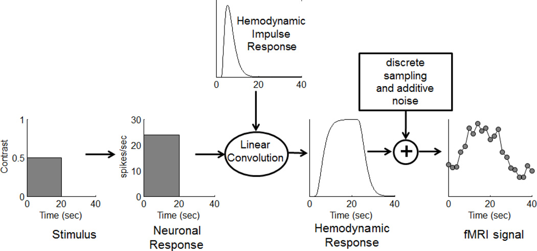
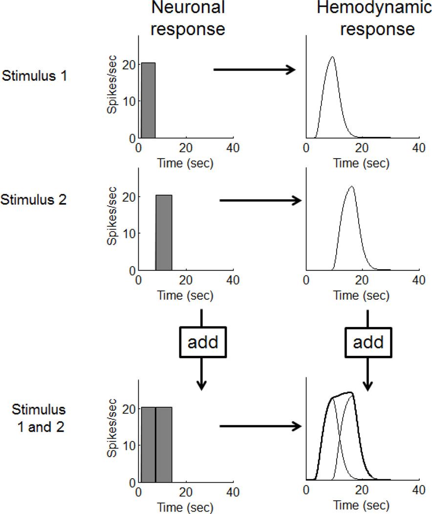
What we were hoping for, and were generally able to support, was a linear transform model for the time-course of the hemodynamic response (figure 1). The linear transform model wasn’t a new idea. In fact, it had already been assumed in previous papers proposing methods for analyzing fMRI data (Bandettini, Jesmanowicz et al. 1993; Friston, Frith et al. 1995). Surprisingly, however, no test of linearity had been conducted to date.

Figure 1.

The linear transform model

The linear transform model posits that the time-course of the fMRI response can be predicted by convolving the time-course of the neuronal response with a hemodynamic impulse response, followed by additive Gaussian noise. For those less familiar with the definition and properties of a linear system, we have provided a brief description in Appendix A.

Why primary visual cortex?

We focused on the primary visual cortex (V1), for a few reasons. First, since feasible applications of retinotopic mapping procedures were still being worked out (in our lab and others), we needed a region of interest that we could find based on structural information. Fortunately for us, V1 lies consistently within the calcarine sulcus. Knowing where to look was particularly important because at that time we only had a single slice (!) of functional data.

Second, we wanted to study an area where we had some understanding of what the neuronal responses might be to a given stimulus. A true test of the linear model should compare the relation between the neuronal responses and the fMRI responses, but of course we were not directly manipulating the neuronal response. Of all areas in the mammalian brain, V1 is perhaps the most studied and well understood. Most important for our purposes, it is well known that nearly all V1 neurons increase their firing rate monotonically with stimulus contrast (Albrecht and Hamilton 1982). We could therefore be reasonably confident that the mean firing rate of neurons in V1 increases monotonically with stimulus contrast. Note that we did not assume that the visual system itself was linear: we included a nonlinear contrast-response function in the linear transform model. We did, however, assume that when a stimulus was presented continuously with a constant contrast that the neuronal responses would likewise be constant over time. That is known to be incorrect because of nonlinearities in neuronal activity including adaptation, something which we dealt with post-hoc in the original paper, and which we discuss further below.

Third, we wanted robust reliable data, and we knew even then that fMRI responses in V1 are stronger and more reliable than most other brain areas – probably due to the relative homogeneity of the neuronal population and to the experimenter’s control over the time-course of the input to that area.

We designed our experiments to test the linear transform model in both the time domain and in the frequency domain (See Appendix A for an explanation of time and frequency domains). The general procedure was to manipulate the intensity and duration of the visual stimulus and measure the time-courses and amplitudes of the fMRI responses in V1. We used two kinds of analyses to test the linear model hypothesis. The first was a non-parametric investigation of the data to see if the responses were consistent with some of the properties of linearity. The second was a brute-force parameterized model fit to the data. Both of these tests were applied to two sets of experiments – one emphasizing the time domain and the other emphasizing the frequency domain.

Time Domain Study

We first tested linearity in the time domain using what is now called a slow event-related design. We simply measured the time-course of the fMRI response to flickering checkerboards of different contrasts and durations. We waited 30 seconds or so between repeated trials to let the hemodynamics recover to baseline. After acquiring several runs across several days, we averaged the time-course of each response from voxels within a hand-drawn region of interest, time-locked to the onset of each stimulus.

Scaling

If the hemodynamic transfer function is linear, then the time-courses of the fMRI response to stimuli for a given duration should vary only by a scale factor with contrast. This follows from the scalability property of a linear system. Note that we are assuming that the time-course of the neuronal response follows the time-course of the stimulus (at least as far as the time-scale of fMRI is concerned). This means that even though the magnitude neuronal response does not scale in proportion to stimulus contrast, the shape of the hemodynamic responses should remain the same across contrasts.

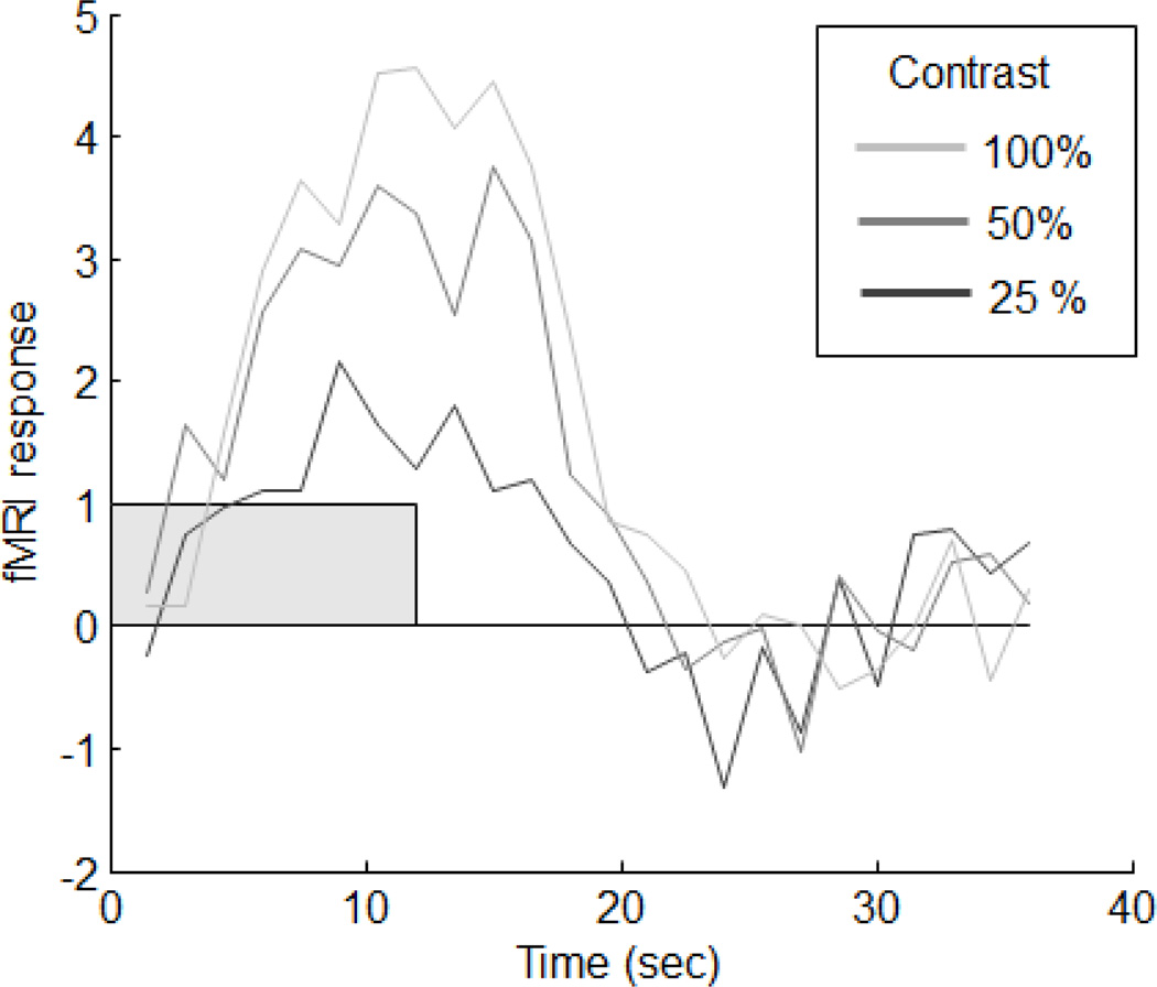
The results were surprisingly clear. The response magnitudes scaled nicely across the three contrasts (25, 50 and 100%). Figure 2 shows an example response from one of the subjects to a 12 second stimulus. Note how the shape of the time-course did not vary – it only scaled with contrast. (Note how these results compare to the predictions of the linear model shown in Appendix A, Figure A1).

Figure 2.

Example of time-contrast separability. The shape of the response to a 12 second stimulus does not vary across the three stimulus contrasts.

Figure A1.

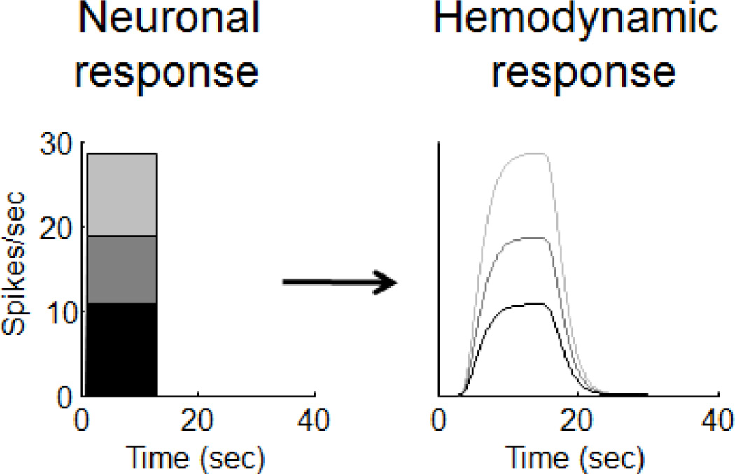
Example of the scaling property. Scaling the size of the input to a linear system scales the size of the output without changing the shape of the response over time.

We called this less-than-perfect scaling time-contrast separability. From a statistical sense it can be thought of as time-contrast independence, in which there is no interaction between the effects of the independent variables of time and contrast. Figures 10 and 11 in the original paper showed how scalability held up for the four durations tested (3, 6, and 24 seconds) for the two subjects.

It is important to point out that we did not find (or expect to find) that the BOLD signal would scale directly with stimulus contrast. Most biological systems show compression for large inputs, so that doubling the strength of the input produces much less than doubling of the output. This is true for the sensory systems and for contrast in particular. It is clearly visible in figure 2 (and figure A1): Doubling the contrast from 50% to 100% produced a scaling of the output, but the scaling was much less than a factor of two. We know that this is true of the underlying neuronal responses so it is not surprising that it is inherited by the hemodynamic responses. But this was not a violation of the linear transformation model, because it is still possible that the BOLD signal is scaling with the underlying (compressed) neuronal response. Time-contrast separability was consistent with a linear system relating the neuronal and hemodynamic responses that was preceded by a nonlinear relationship between stimulus strength and neuronal response. This nonlinear component is termed the contrast-response function, and was easily inferred from our data by plotting the stimulus contrast against the magnitude of the corresponding fMRI response.

Time-contrast separability, or more generally time-stimulus separability, is critical for allowing meaningful data analysis. Suppose, for example, that the vascular system reacted more quickly to a stronger neuronal input, leading to a differently shaped hemodynamic response for high contrast stimuli. This would be a disaster for data analysis since we wouldn’t be able to generate a single template to correlate with our data. We’d be stuck in a circular dilemma in which we’d need to know the strength of the neuronal response to generate the appropriate template time-course which would then be used to detect and estimate the underlying neuronal response.

Additivity

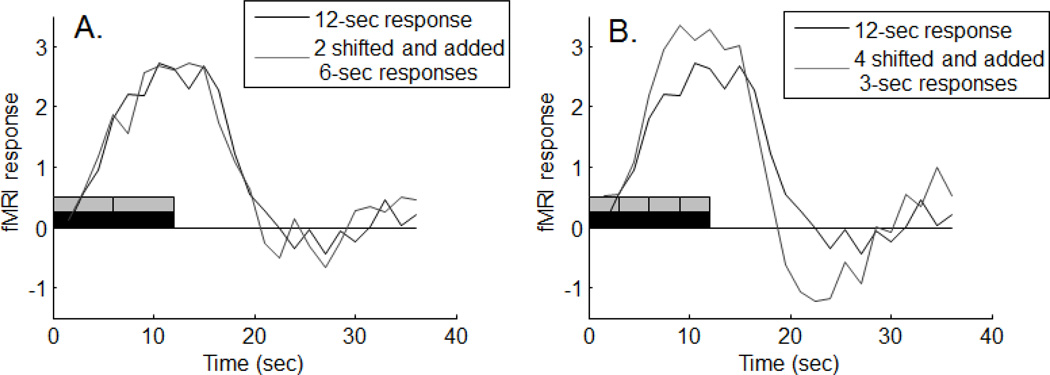
We next tested the property of additivity with the same time-domain data by, for example, treating a 12 second stimulus as two successive 6 second stimuli. If additivity and shift invariance hold, then we should be able to predict the response to the 12 second stimulus by adding two responses to the 6 second stimulus, with the second response shifted by 6 seconds. Figure 3(A) shows an example of this from one of the subjects. Shown in red is the average time course to a 12-second stimulus. The blue curve was generated by adding the response to the 6-econd stimulus to a shifted copy of itself. The red and blue boxes on the time-line represent the time-courses of the stimuli.

Figure 3.

Example of additivity. (A) Response to a 12 second stimulus predicted by the responses to two 6-second stimuli. (B) Response to the same 12 second stimulus predicted by the responses to four 3-second stimuli.

The curves overlap. This means that the sum of the responses to two successive 6-second stimuli was equal to the response to the sum of two successive 6-second stimuli. That is, the results were consistent with the principal of additivity (compare these results with the predictions from the linear transform model shown in Appendix A, Figure A2).

Figure A2.

Example of the additivity property. The response to the sum of two inputs is equal to the sum of the responses to the inputs alone.

Since we used 3, 6, 12, and 24-second stimuli we were able to make a total of 6 predictions (e.g. a 24 second response was predicted by shifting and adding six 3-second responses, etc.). Most of the predictions matched nicely, like the example in figure 3(A).

Figure 3(B) shows what happened when a 3-second responses was used to predict the same 12-second response. The fit wasn’t as good. The shifted and summed 3-second prediction was too large compared to actual response to the 12-second stimulus. This violation of the additivity property was also evident in our parametric fit to the data, which will be described below.

Like scaling, it is not hard to imagine how additivity could have failed for a complex phenomenon like the hemodynamic response, especially considering that the vascular response provides an oversupply of oxygenated blood. Suppose, for example, that once a response to the first stimulus is underway, the vascular response to the second stimulus is not needed, so little additional hemodynamic response is added. The disproportionately large response to the 3-second stimulus might mean that this may actually be the case to some extent. Or it might simply reflect a nonlinearity (such as adaptation) in the neuronal response.

Parameterized fit

So far we have shown support for scaling and additivity using parameter-free analyses of the data. Given this support, we went ahead and fit the entire time-domain data sets with a parameterized version of the linear transform model. The model had two separate parts. The first was a parameterized contrast-response function, and the second was a parameterization of the impulse response function.

The form for the contrast response function was borrowed from the single-unit electrophysiology (Albrecht and Hamilton 1982) and psychophysics (Legge and Foley 1980) literature. The function predicts the relation between stimulus contrast c, and neuronal response r as:

$$r(c)=\frac{a{c}^p}{c^p+\sigma }$$ (1)

This function, called a hyperbolic ratio function or sometimes the Naka-Rushton equation, predicts a decelerating or compressive response as a function of contrast, as is typically seen in single-unit data from the macaque primary visual cortex (Albrecht and Geisler 1991).

For the impulse response function (later called the hemodynamic response function (Friston, Josephs et al. 1998) we chose the Gamma distribution function (not to be confused with the regular Gamma function, Γ, which is an extension of the factorial function for non-integers).

$$h(t)=\frac{{\left(\raisebox{1ex}{$1$}\!\left/ \!\raisebox{-1ex}{$\tau $}\right.\right)}^{(n-1)}{e}^{\left(\raisebox{1ex}{$1$}\!\left/ \!\raisebox{-1ex}{$\tau $}\right.\right)}}{\tau (n-1)!}$$ (2)

The Gamma distribution function has two parameters, n (an integer) and a time-constant, τ. Gamma distribution functions often shows up in the context of linear systems. Perhaps the simplest linear system is one with an exponential impulse response function, which describes any self-equilibrating system that changes over time at a rate proportional to the difference between the current state and the asymptotic state. An RC circuit is an example of a linear system with an exponential impulse response function. The Gamma distribution function is the impulse response function for a cascade of n such exponential systems – that is a series of exponential systems that feed in to the next. Gamma distribution impulse response functions therefore show up in all sorts of models, such as those describing fluid dynamics, heat conduction and membrane potentials.

The first author became aware of the Gamma distribution functions in a linear stage of a model for the temporal properties of the human visual system (Watson 1986). The interested reader should visit this chapter in the Handbook of Perception and Human Performance to see how closely our paper follows Watson’s 1986 working model of the temporal sensitivity of the human visual system. We essentially borrowed Watson’s analysis and applied it at the scale of seconds rather than milliseconds.

The full model predicts the fMRI response as the time course of the stimulus convolved with the Gamma distribution function, scaled by the contrast response function. Time-contrast separability is a simple consequence of the two separate parameterizations for time and contrast. The full parameterized model has a total of five free parameters: two for contrast, two for the Gamma distribution function, and one more describing a delay in the impulse response function. This five parameter model was fit to the fMRI time courses for the three contrasts and four durations using the nonlinear optimization algorithm provided by MATLAB.

The model fit the data from the time-domain study well for both subjects, except that it systematically underestimated the magnitude of the fMRI response for the stimuli having shorter durations. This can be seen in the original paper (figures 10 and 11) where the data points exceed the predicted model curves for the 3-second stimulus. This apparent nonlinearity for brief stimuli was noted above, and has since been replicated in both the visual system (Vazquez and Noll 1998; Birn, Saad et al. 2001) and the auditory system (Robson, Dorosz et al. 1998). The nonlinearity can be quite large; Birn et al (2001) later found that the fMRI response to a 250 msec visual stimuli can be 3–5 times larger than what is expected from a longer stimulus. This has important implications for the interpretation and analysis of rapid event-related fMRI studies that typically use brief stimulus events.

In the original paper we speculated about the possible causes of the relatively large fMRI responses we found for short stimuli. One possibility is a nonlinearity in the function relating neuronal activity to hemodynamic response. But it could also be a purely neuronal effect. For example, transient bursts of neuronal firing occur at the onset and offset of neuronal responses (Albrecht, Farrar et al. 1984; Maddess, McCourt et al. 1988; Bonds 1991). Linear convolution with a typical hemodynamic impulse response function predicts that these transient bursts would have a relatively large influence on brief stimuli because they contribute relatively more to the average response over time.

In a subsequent paper, the first author teamed up with the Bandettini lab at NIH and tested the transient hypothesis by replicating the original fMRI result using stimuli of durations 1, 3 and 6 seconds, but also adding a gradual contrast ramp that is was intended to reduce the strength of the onset and offset neuronal transients. A parallel MEG study with the same subjects and stimuli showed that the ramps did effectively reduce the transient neuronal activity. However, the nonlinearity in the BOLD signal remained (Tuan, Birn et al. 2008).

A related neuronal explanation is long-term adaptation. It is well known that V1 neurons reduce their responses over time to long-duration stimuli (e.g. Bonds, 1991). Our flickering checkerboards, lasting up to 24 seconds, are exactly the sort of stimuli used in adaptation experiments. In the original paper, we showed that a better fit was obtained by incorporating a model of neuronal adaptation.

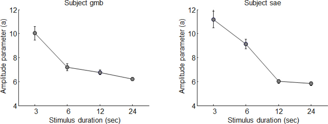
A reanalysis of our original data provides further support for this idea. We have re-fit the original data with the linear transform model, but allowed four different amplitudes (the parameter a in equation 1 above) to vary for the four different stimulus durations while the other parameters of the modified model were held fixed to the original best-fitting parameters. Figure 4 shows a plot of the best-fitting amplitude parameters for each of the four stimulus durations for the two subjects. Error bars represent bootstrapped estimates of parameter variability based on resampling using the standard errors of the original data.

Figure 4.

Reanalysis of the time-domain results. The amplitude parameters were allowed to vary for each of the four durations, showing how the fMRI responses to shorter stimuli are relatively stronger than the responses to longer stimuli.

The reanalysis shows something not apparent in the original figures; the best-fitting amplitude parameters decrease across the entire range of stimulus durations. The effect seems to decay with duration in an exponential fashion and a time constant of seconds, which is remarkably consistent with the time-course of adaptation seen in electrophysiology (Bonds 1991) and psychophysical experiments (Greenlee, Georgeson et al. 1991). For a similar analysis of the nonlinearity using event-related designs, see (Heckman, Bouvier et al. 2007)

Frequency Domain Study

As described in Appendix A, another way to investigate linearity is in the frequency domain using sinusoidally modulating stimuli. Ideally we would have liked to invoke a sinusoidal neuronal response, but this was not possible without knowing the exact relation between stimulus contrast and neuronal response. Instead we chose to use a blocked-design in which the stimuli turned on and off as a square wave over time. The actual stimulus was a square-wave in space (vertically oriented bars of flickering checkerboards) that slowly drifted horizontally at different rates. The time-course of stimulation at any given point in space therefore turned on and off at a rate related to the speed of the drift. We chose this design over a full-field on/off stimulus because we were trying to minimize the effects of blood vessels that pool across large regions of cortex. The overall stimulation across the visual field in our design remained roughly constant, unlike the case for a full-field stimulus. It is interesting to note that the effects of draining veins on fMRI signals was a major concern back then, but receives relatively little attention today – yet the problem remains. Indeed, a recent study supports the idea that discrepancies in the literature on retinotopic maps in visual area V4 may be due an artifact caused by the transverse sinus that passes near V4 in some subjects (Winawer, Horiguchi et al. 2010).

In our study, we measured fMRI responses to drifting bars with temporal periods of 10, 15, 30 and 45 seconds using five contrasts ranging from about 3% to 100%. Our dependent measure was the amplitude of the fMRI response at the fundamental frequency of modulation. With a linear system, this measure should be proportional to the on/off amplitude of the underlying neuronal response (See Appendix A for an explanation). Not surprisingly, the amplitudes of the responses decreased with decreasing temporal period (or increasing temporal frequency) due to the low-pass nature of the hemodynamic transformation.

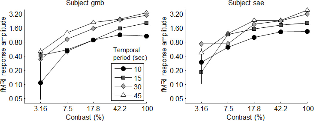
More importantly, the results again showed strong support of time-contrast separability, meaning that changing the temporal period had only a scaling influence on the shape of the contrast-response (see the original figure 6). Replotting the original results on a log-response axis emphasizes this point (Figure 5). Curves that are multiple scales of each other (as predicted by time-contrast separability) should be parallel on a log-amplitude axis. The curves in figure 5 are roughly parallel with no systematic deviations in shape across stimulus contrast.

Figure 5.

Frequency-domain results plotted on a log-response axis to illustrate time-contrast separability.

Parameterized fit

We fit the same linear transform model to the data from the frequency domain experiment and found similar parameter values as for the time-domain data. This was important because though the experimental designs and dependent measures were quite different, the same model should fit both data sets with roughly the same parameters.

Noise

A final important result of our study related to the noise found in fMRI data. In the linear transform model, noise is added after the convolution stage (see figure 1). This makes specific predictions about the fMRI response that can best be thought of in the frequency domain. Truly additive and independent Gaussian noise (where an independent random number drawn from a normal distribution is added to the response at every time point) contains sinusoids at all frequencies with roughly equal amplitudes. If Gaussian noise is added after the linear transform, then the Fourier transform of the output should look like a signal (amplitudes at frequencies related to the input) plus a flat spectrum of amplitudes across all frequencies. If, however, noise was added before the linear transform, then the higher frequency components of the noise should be attenuated by the low-pass process of the hemodynamics.

We found that the noise spectrum of our frequency-domain study was relatively flat (our original figure 9). This has important implications for those using deconvolution to estimate the hemodynamic response function from event-related experiments, because deconvolution is essentially linear regression which assumes additive Gaussian noise. It also means filtering fMRI data with a low-pass temporal filter is a good idea, since the variability in the fMRI time-course at high temporal frequencies is likely due to stimulus-independent noise factors.

A side note- subject gmb showed a splattering of noise around the 3–6 second temporal period, which is around the period of respiration (See figure 9B in the original publication). In retrospect, this respiratory artifact is probably not a hemodynamic issue but was probably related to the physical stimulus. We projected our images from the foot of the scanner table over the subjects’ chest on to a screen just at the subject’s neck. The rising and falling of subject gmb’s chest may have periodically blocked the bottom of the image, leading to a temporal modulation of the visual signal. Subject sae did not have this problem.

Impact

Our results supported the linear transform model well enough for us to confidently move on to quantitative studies of the human visual system. As stated above, the results satisfied our main concern that there might be an interaction between the strength of the neuronal response and the shape of the hemodynamic response.

Our plans at the time were to use our knowledge of linearity to analyze results from blocked –design experiments. This is why much of our paper focused on the frequency-domain experiment and results. With linearity, we could be confident that the amplitude of the fMRI signal in a blocked design experiment was proportional to the amplitude of the underlying neuronal response. We then went on and applied blocked-designs in a variety of studies, using the amplitude of the Fourier transform at the stimulus frequency as our measure of neuronal response (e.g. Demb, Boynton et al. 1997; Demb, Boynton et al. 1998; Boynton, Demb et al. 1999; Gandhi, Heeger et al. 1999; Heeger, Boynton et al. 1999; Wandell, Poirson et al. 1999).

What we did not anticipate was the impact that our paper would have on the emerging method of rapid event-related designs (see Huettel in this issue) in which brief stimuli are presented close enough in time for their responses to overlap. In a typical event-related fMRI experiment, different types of events or conditions are presented in a pseudo random order, resulting in a time-varying fMRI signal that contains the sum of responses to individual events. The hemodynamic response function for each event type is then found that best-predicts the fMRI results when convolved with the time-course of the stimulus (Dale 1999). Clearly this deconvolution process relies heavily on the assumption of linearity. Alternatively, a canonical hemodynamic response function is assumed which, when convolved with the stimulus time-course, produces a predicted fMRI time-course that can be correlated with individual voxel time-courses. These correlations provide a statistical parameter map for localizing event-related activity.

An anecdotal note: we actually tried to test the linear transform model by measuring the fMRI response to a stimulus that followed a complicated time-course (ramping up and down in contrast, turning on and off, etc.) In theory, we should have been able to use our model and best-fitting parameters to the original data to predict the resulting fMRI time course in V1. Unfortunately we didn’t have enough signal-to-noise in our data set to provide a convincing figure for the paper. Perhaps this is why we went on to using the blocked design in future studies instead of pursuing similar overlapping designs, including event-related ones.

Note that brief stimulus presentations like those used in event-related fMRI appears to show the greatest violation of the linearity assumption. However, the reanalysis above (see figure 4) shows that another way to look at our results is that linearity fails for longer stimulus durations (due perhaps to neuronal adaptation). The over-prediction of our original model in fits for short stimulus presentations was probably simply because the model placed more weight on the longer-stimulus duration signals since they contained more data points.

Over the past 15 years much effort has been put into studying the biological basis of the hemodynamic coupling process. A second impact of our paper has been to provide a framework for some of these studies, particularly for correlative studies that compare more direct measures of neuronal activity to more direct measures of blood flow and oxygenation. Perhaps the most well-cited example of this is the study by (Logothetis, Pauls et al. 2001) that simultaneously measured the BOLD signal and electrophysiological responses in the monkey visual cortex. This effort led to the suggestion that the BOLD signal is more linearly related to local field potentials than spikes, though both are good predictors of the BOLD signal. A very recent example of a correlative study is (Kahn, Desai et al. 2011) that used a combination of optogenetics to stimulate the somatosensory cortex in mice while measuring the BOLD signal and electrophysiological recordings.

Another recent example is a study by Sirotin and Das. They measured simultaneously spiking activity and intrinsic optical signals. They found that there was a component of the hemodynamic responses that was time-locked to the stimulus presentations but not differentially responsive to the different stimulus conditions. They found likewise that there was such a baseline component in the spiking activity. The two baseline components (spiking and hemodynamic) were not related to one another (Sirotin and Das, Nature, 2009). But after removing each of the two baseline response components, the residual hemodynamic responses are very tightly linked with spiking activity, such that the time courses of the hemodynamic responses evoked by different stimulus contrasts are very well fit as a shift-invariant linear transform of the firing rates (A. Das, personal communication). Temporal summation experiments, much like our additivity ones, showed that once again, the hemodynamic coupling process is remarkably linear.

Another unanticipated impact of our paper is that the best-fitting parameters from our study are often used to model the hemodynamic response in a variety of studies. This is probably because certain software packages, such as BrainVoyager have a model of the hemodynamic response with parameters set to those in our paper. Though the parameters are adjustable, many users just use the default parameters. The two subjects (gmb an sae) were both authors, so it is amusing to note how the authors’ brains contributed to this paper in more than one way. But using these exact parameters is dangerous because it is well known that the hemodynamic response function varies significantly across subjects and brain areas e.g. (Aguirre, Zarahn et al. 1998). With our extremely small sample size of two subjects, it doesn’t seem wise to use our parameters for estimates of the population. Indeed, given that the hemodynamic response varies with age, (Kannurpatti, Motes et al. 2010) the parameters from this paper are probably not even appropriate for our own, now middle-aged brains!

Appendix A

In this appendix we define the properties of a linear system in the context of the transformation between a neuronal response and the BOLD signal.

A linear system satisfies the two properties of scaling and additivity. For our model, we also assume a third property, shift invariance.

Scaling

For a system operating in the time domain, scaling means that the time-course of the output directly scales with the strength of the input. For the case of a hemodynamic transform, L, we’ll define the input as a neuronal response over time, n(t), and the hemodynamic response H(t) as the output of the system:

$$H\mathit{(}t\mathit{)}=L\mathit{[}n\mathit{(}t\mathit{)}\mathit{]}$$ (A1)

For scaling to hold, if we multiply our input n(t) by a factor k, then:

$$L\mathit{[}kn\mathit{(}t\mathit{)}\mathit{]}\mathit{]}=kL\mathit{[}n\mathit{(}t\mathit{)}\mathit{]}=kH\mathit{(}t\mathit{)}$$ (A2)

The new output is equal to the original output multiplied by the scale factor k.

In the case of the hemodynamic response, the slow, delayed time-course of the output is very different than the shape of the input, and we are interested in whether a linear system relates the two. If this system shows scaling, then when the input is scaled the shape of the output will always remain the same except that it is scaled by the same factor. Figure A1 illustrates the scaling property for an example hemodynamic response to three neuronal inputs identical in time, but with different strengths. Shown are three neuronal responses and the predicted hemodynamic responses over time, each scaled in proportion to their corresponding neuronal response.

Additivity

The property of additivity states that given two inputs, the response to the sum of the inputs is equal to the sum of the responses to each of the inputs alone. For our system L, given two inputs n₁(t) and n₂(t):

$$L\mathit{[}{n}_{\mathit{1}}\mathit{(}t\mathit{)}+n_{\mathit{2}}\mathit{(}t\mathit{)}\mathit{]}=L\mathit{[}{n}_{\mathit{1}}\mathit{(}t\mathit{)}\mathit{]}+L\mathit{[}{n}_{\mathit{2}}\mathit{(}t\mathit{)}\mathit{]}$$ (A3)

For the hemodynamic response, the additivity property is best illustrated for two neuronal responses that follow closely in time. If they fall within a few seconds of each other, the output hemodynamic response to the first input will still be ongoing when the hemodynamic response to the second input begins. The additivity principal says that this second hemodynamic response should simply add to the first response, without interacting in any way.

Figure A2 shows an example of how, for a linear shift-invariant system, the hemodynamic responses to two successive 6-second inputs is identical to the sum of the responses to a 6-second input added to the same 6-second input delayed by 6 seconds. That is, you can either add the inputs and then measure the response, or you can measure the responses to the individual stimuli first and then add them.

Shift Invariance

The additional property of shift invariance is also assumed in the linear transform model. Shift invariance means that the hemodynamic response to a later input neuronal response should look just like the response to an earlier, identical input, but shifted in time by the delay between the two inputs.

Convolution

The two properties of scaling and additivity combine in a very powerful way. Consider an arbitrary neuronal time-series n(t). We can think of this time-series a sequence of shifted brief impulses δ(t), each scaled accordingly:

$$n(t)={\displaystyle \sum _i{k}_i\delta (t-i)}$$ (A4)

The response to an impulse input is called (naturally) the impulse response function,

$$H(t)=L[\delta (t)]$$ (A5)

Then by the properties of additivity and scaling, the response to the arbitrary input is:

$$L\left[{\displaystyle \sum _i}{k}_i\delta (t-i)\right]={\displaystyle \sum _i}{k}_{i}L[\delta (t-i)]={\displaystyle \sum _i}{k}_{i}H(t-i)$$ (A6)

That is, the response is the sum of shifted and scaled responses to the impulse.

The above argument shows that the impulse response function completely characterizes a linear system, because it can be used to predict the response to any input. Of course, characterizing a time-series as a sum of discrete scaled impulses is only an approximation, but the above argument holds for any size impulse, no matter how small. In the limit, the impulse response function is defined to be the response to an infinitely short input.

Figure A3 shows a hemodynamic response to an arbitrary neuronal time-series defined as a sequence of scaled impulses. Each of these brief impulses produces its own scaled response, and the response to the entire time series is simply the sum of these individual scaled responses.

Figure A3.

Combining scaling and additivity. The response to any arbitrary stimulus can be predicted by the summed and shifted responses to an impulse input.

This process of shifting and scaling a series of impulse responses to predict a linear system’s response to an arbitrary input is called convolution. It is possible to go the other way and estimate the impulse response given a linear system’s input and measured output. The reverse process is called deconvolution and is used in the analysis of event-related fMRI experiments.

Frequency response

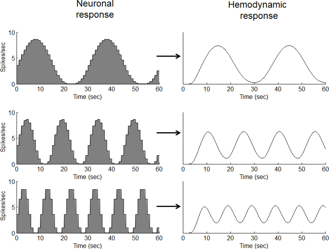
A second way to characterize a linear system is to work in the frequency domain, which is to think about how the system transforms inputs that vary sinusoidally over time. Given a system that obeys scaling and additivity, the response to a sinusoidal input is also a sinusoid of the same frequency, though possibly shifted in phase. Remarkably, this is only true for sinusoids (technically, it’s true for all complex exponentials which includes sinusoids), and is true for any shaped impulse response function. Figure A4 shows how a linear hemodynamic system should respond to sinusoidal inputs of varying frequency (temporal periods of 30, 15 and 10 seconds). Note how the frequency of the output matches the frequency of the input.

Figure A4.

The response of a linear system to a sinusoidal input is equal to a sinusoid of the same frequency, only scaled in amplitude and delayed in time.

According to the Fourier theorem, any arbitrary time-series can be described as a sum of sinusoids, each having a specific amplitude frequency and phase. Using an argument like the one above for convolution, if we know how a linear system shifts and scales each of these sinusoids then we can predict how the linear system will transform any arbitrary input, since the output will simply be the sum of shifted and scaled sinusoids that composed the input.

The way a linear system transforms a series of sinusoids is called the frequency response function. Looking at figure A4, it can be seen that the amplitude of the response is decreasing as the frequency of the input increases (or as the period decreases). There is also a specific phase delay for each frequency, but here we’ll focus only on amplitudes. This illustrates the typical low-pass property of the hemodynamic response; the higher the frequency of the input, the lower the relative amplitude of the output of the system.

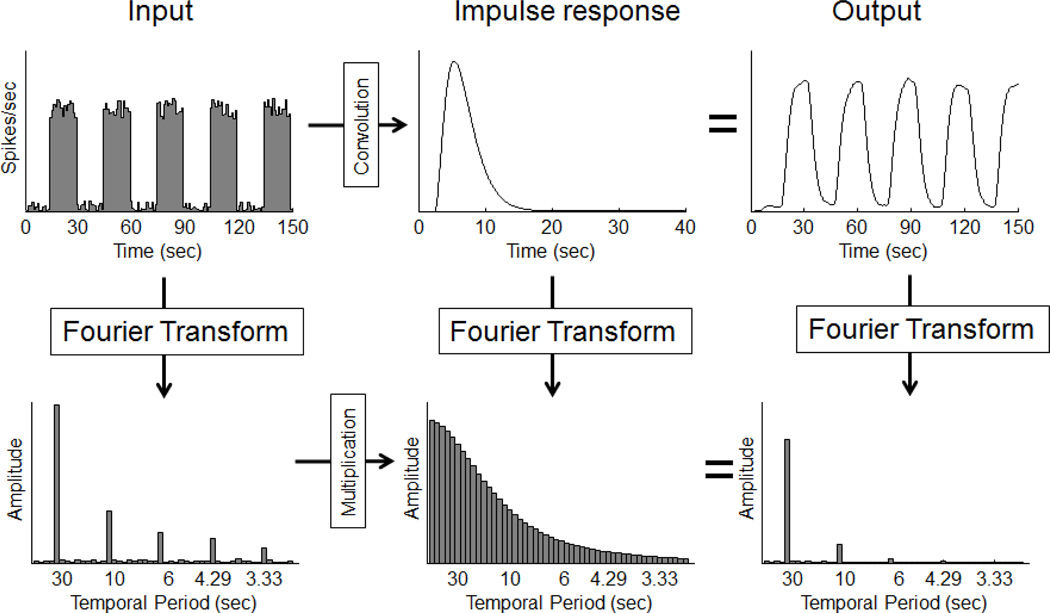
It is not hard to show that there is a direct relationship between the impulse response function for a linear system and the corresponding frequency response function. This is the basis of the convolution theorem which states that convolution in the time domain is the same is multiplying in the frequency domain. That is, the Fourier transform of the output of a linear system is equal to the product of the Fourier transforms of the input and the impulse response function.

Figure A5 illustrates the Fourier theorem for a blocked-design experiment. The input to the system is an on/off blocked design with a 30 second period (period = 1/frequency), plus some additive neuronal noise. It is assumed in this simulation that the input neuronal responses are turned on and off following a square wave. The top row shows the linear system operating in the time domain by convolving the input neuronal response with the impulse response function. The output is a smoothly varying, roughly sinusoidal modulation. Now consider the Fourier transform of the neuronal input (in the bottom left of figure A5). It shows that to build a square-wave signal, we need to add discrete sinusoidal components of increasing frequency and decreasing amplitude. If our temporal period is P seconds, then the periods we need are P/n for n= 1, 3, 5, 7,… and the corresponding amplitudes are 4π/n. In our example of a square wave with a 30 second period, we need to add sinusoids of decreasing amplitudes starting with a sinusoid with a period of 30 seconds (called the fundamental period), followed by sinusoids having periods of 30/3=10, 30/5 = 6, 30/7 = 4.29, 30/9 = 3.33 seconds and so on.

Figure A5.

The convolution theorem: For a linear system, convolution in the time domain is equivalent to multiplication in the frequency domain.

We can think of a linear system as working on each of these sinusoidal components independently. To see how the hemodynamics affect the input, we can look at the Fourier transform of the impulse response function, shown in the middle of the bottom row in figure A5. This graph shows how sinusoids are scaled by each input frequency, and specifically, how the amplitude of the output decreases with increasing frequency (decreasing temporal period). To predict the output of the system to our square-wave input, we simply multiply each of the amplitudes in the stimulus by their corresponding value in the frequency response (multiplication is actually done with complex numbers which takes into account both amplitude and phase).

The Fourier transform of the resulting output is shown in the bottom right of figure A5. The already decreasing amplitudes in the input decrease more rapidly in the output due to the low-pass nature of the impulse response function. The higher frequencies in the input serve to “square-off” the fundamental 30-second period sinusoid. Attenuating these higher frequencies by the hemodynamic linear system causes the output to look less square and more sinusoidal. For this example, the fMRI response to a 30 second period input has only a small 10-second period component and negligible higher frequency components. Nearly all of the response is at the fundamental frequency. This means that the analysis of results from a blocked-design experiment using a 30-second period can focus on just the amplitude of the 30-second period Fourier component without throwing out much information in the signal.

Note also that the property of scaling applies in the frequency domain as well. Doubling the amplitude of a sinusoidal input doubles the amplitude of the sinusoidal output. In the early days of fMRI, the majority of studies used a standard blocked-design paradigm in which two stimulus conditions alternated back and forth throughout a scan at an even period. Using an on/off period of 30 seconds or so, the resulting fMRI signal should modulate in a roughly sinusoidal manner. With scaling, the amplitude of the sinusoidal fMRI signal can serve as a measure of neuronal activity (e.g. Boynton, Demb et al. 1999; Gandhi, Heeger et al. 1999; Heeger, Boynton et al. 1999). That is, given a linear hemodynamic transform, the amplitude of the sinusoidal output should be proportional to the amplitude of the underlying neuronal response. A common application of the blocked design is for phase-encoded retinotopic mapping experiments (See Engel, this issue). The analysis of these experiments only relies on the response at the fundamental frequency of the stimulus. In analyzing these experiments, a sinusoidal model of the BOLD signal was sufficient due to the low-pass nature of the hemodynamic impulse response function (Engel, Rumelhart et al. 1994).

References

- Aguirre GK, Zarahn E, et al. The variability of human, BOLD hemodynamic responses. Neuroimage. 1998;8(4):360–369. doi: 10.1006/nimg.1998.0369. [DOI] [PubMed] [Google Scholar]
- Albrecht DG, Farrar SB, et al. Spatial contrast adaptation characteristics of neurones recorded in the cat's visual cortex. J Physiol (Lond) 1984;347:713–739. doi: 10.1113/jphysiol.1984.sp015092. [DOI] [PMC free article] [PubMed] [Google Scholar]
- Albrecht DG, Geisler WS. Motion selectivity and the contrast-response function of simple cells in the visual cortex. Vis Neurosci. 1991;7(6):531–546. doi: 10.1017/s0952523800010336. [DOI] [PubMed] [Google Scholar]
- Albrecht DG, Hamilton DB. Striate cortex of monkey and cat: contrast response function. J Neurophysiol. 1982;48(1):217–237. doi: 10.1152/jn.1982.48.1.217. [DOI] [PubMed] [Google Scholar]
- Bandettini PA, Jesmanowicz A, et al. Processing strategies for time-course data sets in functional MRI of the human brain. Magn Reson Med. 1993;30(2):161–173. doi: 10.1002/mrm.1910300204. [DOI] [PubMed] [Google Scholar]
- Birn RM, Saad ZS, et al. Spatial heterogeneity of the nonlinear dynamics in the FMRI BOLD response. Neuroimage. 2001;14(4):817–826. doi: 10.1006/nimg.2001.0873. [DOI] [PubMed] [Google Scholar]
- Bonds AB. Temporal dynamics of contrast gain in single cells of the cat striate cortex. Vis Neurosci. 1991;6(3):239–255. doi: 10.1017/s0952523800006258. [DOI] [PubMed] [Google Scholar]
- Boynton GM, Demb JB, et al. Neuronal basis of contrast discrimination. Vision Res. 1999;39(2):257–269. doi: 10.1016/s0042-6989(98)00113-8. [DOI] [PubMed] [Google Scholar]
- Boynton GM, Engel SA, et al. Linear systems analysis of functional magnetic resonance imaging in human V1. J Neurosci. 1996;16(13):4207–4221. doi: 10.1523/JNEUROSCI.16-13-04207.1996. [DOI] [PMC free article] [PubMed] [Google Scholar]
- Dale AM. Optimal experimental design for event-related fMRI. Hum Brain Mapp. 1999;8(2–3):109–114. doi: 10.1002/(SICI)1097-0193(1999)8:2/3<109::AID-HBM7>3.0.CO;2-W. [DOI] [PMC free article] [PubMed] [Google Scholar]
- Demb JB, Boynton GM, et al. Brain activity in visual cortex predicts individual differences in reading performance. Proc Natl Acad Sci U S A. 1997;94(24):13363–13366. doi: 10.1073/pnas.94.24.13363. [DOI] [PMC free article] [PubMed] [Google Scholar]
- Demb JB, Boynton GM, et al. Functional magnetic resonance imaging of early visual pathways in dyslexia. J Neurosci. 1998;18(17):6939–6951. doi: 10.1523/JNEUROSCI.18-17-06939.1998. [DOI] [PMC free article] [PubMed] [Google Scholar]
- Engel SA, Rumelhart DE, et al. fMRI of human visual cortex. Nature. 1994;369(6481):525. doi: 10.1038/369525a0. [DOI] [PubMed] [Google Scholar]
- Friston KJ, Frith CD, et al. Characterizing evoked hemodynamics with fMRI. Neuroimage. 1995;2(2):157–165. doi: 10.1006/nimg.1995.1018. [DOI] [PubMed] [Google Scholar]
- Friston KJ, Josephs O, et al. Nonlinear event-related responses in fMRI. Magn Reson Med. 1998;39(1):41–52. doi: 10.1002/mrm.1910390109. [DOI] [PubMed] [Google Scholar]
- Gandhi SP, Heeger DJ, et al. Spatial attention affects brain activity in human primary visual cortex. Proc Natl Acad Sci U S A. 1999;96(6):3314–3319. doi: 10.1073/pnas.96.6.3314. [DOI] [PMC free article] [PubMed] [Google Scholar]
- Greenlee MW, Georgeson MA, et al. The time course of adaptation to spatial contrast. Vision Res. 1991;31(2):223–236. doi: 10.1016/0042-6989(91)90113-j. [DOI] [PubMed] [Google Scholar]
- Heckman GM, Bouvier SE, et al. Nonlinearities in rapid event-related fMRI explained by stimulus scaling. Neuroimage. 2007;34(2):651–660. doi: 10.1016/j.neuroimage.2006.09.038. [DOI] [PMC free article] [PubMed] [Google Scholar]
- Heeger DJ, Boynton GM, et al. Motion opponency in visual cortex. J Neurosci. 1999;19(16):7162–7174. doi: 10.1523/JNEUROSCI.19-16-07162.1999. [DOI] [PMC free article] [PubMed] [Google Scholar]
- Kahn I, Desai M, et al. Characterization of the Functional MRI Response Temporal Linearity via Optical Control of Neocortical Pyramidal Neurons. J Neurosci. 2011;31(42):15086–15091. doi: 10.1523/JNEUROSCI.0007-11.2011. [DOI] [PMC free article] [PubMed] [Google Scholar]
- Kannurpatti SS, Motes MA, et al. Neural and vascular variability and the fMRI-BOLD response in normal aging. Magn Reson Imaging. 2010;28(4):466–476. doi: 10.1016/j.mri.2009.12.007. [DOI] [PMC free article] [PubMed] [Google Scholar]
- Legge GE, Foley JM. Contrast masking in human vision. J Opt Soc Am. 1980;70(12):1458–1471. doi: 10.1364/josa.70.001458. [DOI] [PubMed] [Google Scholar]
- Logothetis NK, Pauls J, et al. Neurophysiological investigation of the basis of the fMRI signal. Nature. 2001;412(6843):150–157. doi: 10.1038/35084005. [DOI] [PubMed] [Google Scholar]
- Maddess T, McCourt ME, et al. Factors governing the adaptation of cells in area-17 of the cat visual cortex. Biol Cybern. 1988;59(4–5):229–236. doi: 10.1007/BF00332911. [DOI] [PubMed] [Google Scholar]
- Robson MD, Dorosz JL, et al. Measurements of the temporal fMRI response of the human auditory cortex to trains of tones. Neuroimage. 1998;7(3):185–198. doi: 10.1006/nimg.1998.0322. [DOI] [PubMed] [Google Scholar]
- Tuan AS, Birn RM, et al. Differential transient MEG and fMRI responses to visual stimulation onset rate. International Journal of Imaging Systems and Technology. 2008;18(1):17–28. [Google Scholar]
- Vazquez AL, Noll DC. Nonlinear aspects of the BOLD response in functional MRI. Neuroimage. 1998;7(2):108–118. doi: 10.1006/nimg.1997.0316. [DOI] [PubMed] [Google Scholar]
- Wandell BA, Poirson AB, et al. Color signals in human motion-selective cortex. Neuron. 1999;24(4):901–909. doi: 10.1016/s0896-6273(00)81037-5. [DOI] [PubMed] [Google Scholar]
- Watson AB. Temporal Sensitivity. In: Boff, et al., editors. Handbook of perception and human performance. Vol. 1. New York: Wiley; 1986. [Google Scholar]
- Winawer J, Horiguchi H, et al. Mapping hV4 and ventral occipital cortex: the venous eclipse. J Vis. 2010;10(5):1. doi: 10.1167/10.5.1. [DOI] [PMC free article] [PubMed] [Google Scholar]