Abstract
Input function noise contributes to model-predicted values and should be accounted for during parameter estimation. This problem has been examined in the context of PET data analysis using a noisy image-derived arterial input function. Huesman and Mazoyer (1987) incorporated the effect of error in the measured input function into the objective function and observed a subsequent improvement in the accuracy of parameters estimated from a kinetic model of cardiac blood flow. Such a treatment has not been applied to the reference region models commonly used to analyze dynamic positron emission tomography data with receptor-ligand tracers. Here, we propose a strategy for selection of weighting factors that accounts for noise in the reference region input function and test the method on two common formulations of the simplified reference tissue model. We present a simulation study which demonstrates that the proposed weighting approach improves the accuracy of estimated binding potential at high noise levels and when the reference tissue and target regions of interest are of comparable size. In a second simulation experiment we show that using a small, homogeneous reference tissue with our weighting technique may have advantages over input functions derived from a larger (and thus less noisy), heterogeneous region with conventional weighting. A comparative analysis of clinical [11C]flumazenil data found a small but significant increase in estimated binding potential when using the proposed weighting method, consistent with the finding of reduced negative bias in our simulation study. The weighting strategy described here accounts for noise in the reference region input function and may improve the performance of the SRTM in applications where data are noisy and the reference region is relatively small. This technique may offer similar benefits to other models using reference region inputs, particularly those derived from the SRTM.
Keywords: kinetic modeling, neuroreceptors, parameter estimation, positron emission tomography, reference region, weighting factors
1. Introduction
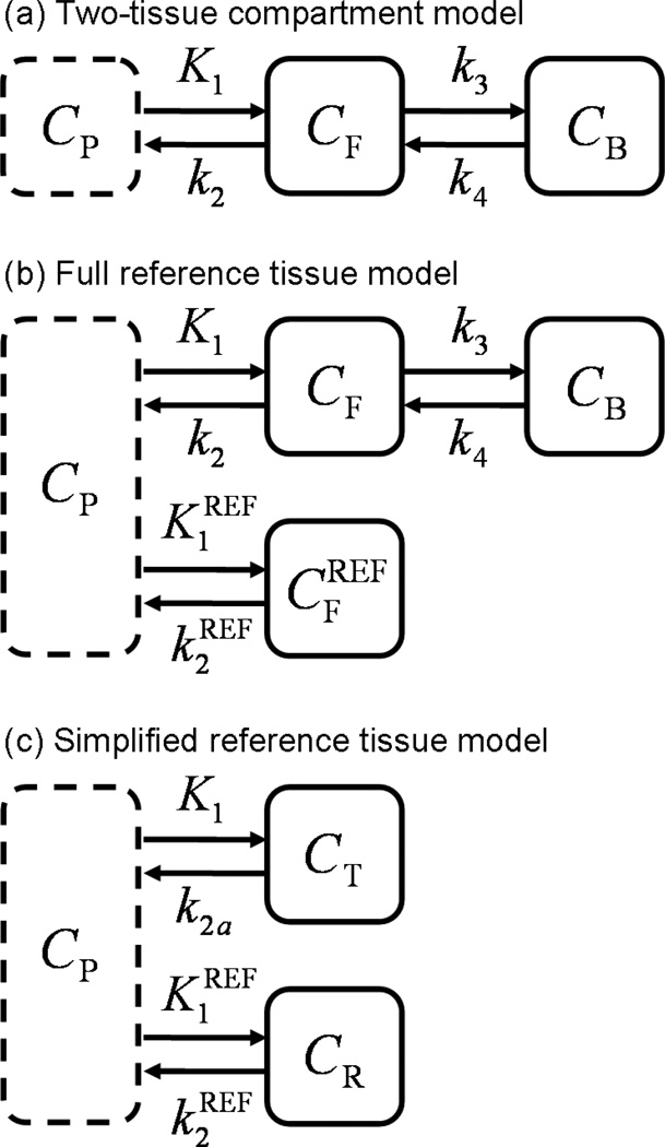
Positron emission tomography (PET) imaging with receptor-ligand tracers has been used extensively to study neuroreceptor density and distribution in vivo. Quantification is typically achieved by calculation of binding potential (BPND), which reflects the equilibrium ratio of specific binding to non-displaceable tracer uptake and serves as an index of receptor availability (see (Innis et al. 2007) for review). BPND was first introduced to the imaging community as an outcome of the two-tissue compartment model (Mintun et al. 1984) (see Figure 1(a)). This model reflects the transfer of tracer molecules between distinct states (i.e., suspended in plasma, free in tissue, or bound to receptors) over time. Using a measured arterial input function one can determine the rate constants describing these transitions. BPND can then be calculated from the estimated model parameters.
Figure 1.
Compartmental models commonly applied to dynamic receptor-ligand PET data. (a) The two-tissue compartment model uses a plasma input function and expresses tracer kinetics in terms of transitions between plasma (CP), free (CF) and bound (CB) states. (b) The full reference tissue model uses the two-tissue model to describe the target region and derives the input function from data acquired in a reference region . (c) The simplified reference tissue model uses a reference region input and collapses the two tissue compartments of the target region into a single apparent compartment (CT).
The full reference region model (Blomqvist et al. 1990, Cunningham et al. 1991) (see Figure 1(b)) derives the input function to the two-tissue compartment model from image data measured in a reference region devoid of receptors. The full reference tissue model eliminates the need for arterial blood sampling, significantly reducing the cost, complexity, and invasiveness of experiments. However, the computational burden of the requisite non-linear data fitting prohibits voxel-by-voxel analysis and parameter identifiability is often unsatisfying (Lammertsma & Hume 1996, Gunn et al. 1997).
The simplified reference tissue model (SRTM) (Lammertsma & Hume 1996) reduces the number of estimated parameters by collapsing the two tissue compartments of the target region into a single apparent compartment as depicted in Figure 1(c). The reduction in number of unknown variables improves parameter identifiability. Computation time is also decreased, but remains formidable because nonlinear parameter estimation is still required. Two common implementations of the SRTM that greatly improve its computational efficiency are the basis function method (BFM) (Gunn et al. 1997) and the multilinear reference tissue model (MRTM) (Ichise et al. 2003) (also derived independently by (Alpert et al. 2003, Zhou et al. 2003)).
The BFM and MRTM parameters are typically obtained by weighted least squares estimation, with each residual (i.e., the difference between measured and model predicted values) weighted according to an approximation of the variance of the corresponding target region PET datum. Weighted least squares is recommended when measurements are not uniformly reliable, as is the case for dynamic PET data. Each squared residual term in the objective function should be normalized by a factor proportional to its variance in order to construct an unbiased estimator. Selecting these weights based solely on the variance of the target region data implicitly assumes that the model predictions do not contribute to the uncertainty of the residuals. The measured input function must be noiseless to satisfy this condition. Fitting the input data to a smooth curve prior to analysis is insufficient because statistical uncertainties propagate from the estimated input function parameters to the model-predicted target region values (Huesman & Mazoyer 1987). If the assumption of an exact input function is not valid, then the weighting factors for each residual are incorrect. Improper selection of weights introduces error into the objective function (Spilker & Vicini 2001).
Huesman and Mazoyer examined the problem of noisy image-derived arterial input functions on the analysis of 82Rb cardiac PET data with a blood flow model (Huesman & Mazoyer 1987). They incorporated the uncertainty attributable to input function noise into the covariance matrix used to weight the residuals during parameter estimation, a method later proven (Huesman 1997) to be mathematically equivalent to extending the objective function with parameters describing the noisy input data (Chen et al. 1991, Chiao et al. 1994). Their approach produced a reduction in the bias of estimated parameters and a moderate improvement in their precision. Previous studies have evaluated the choice of weights for SRTM (Muzic & Christian 2006, Thiele & Buchert 2008, Tomasi et al. 2008a) but did not address the effect of noise in the reference region data. To our knowledge, the reference region PET models have not been scrutinized with respect to the proper assignment of weighting factors given a noisy input function, although the potential need to do so has been recognized in the literature (Aston et al. 2000, Ichise et al. 2003, Zhou et al. 2003).
The purpose of the present work is to adapt the method of Huesman and Mazoyer to the BFM and MRTM implementations of the SRTM and to test its effect on quantification of binding potential. The BFM and MRTM models have received widespread application and the SRTM has inspired numerous extensions (Wu & Carson 2002, Alpert et al. 2003, Ichise et al. 2003, Zhou et al. 2003, Zhou et al. 2006, Ichise et al. 2008, Tomasi et al. 2008b, Møller et al. 2009, Ikoma et al. 2009, Normandin et al. (in press)) to which this weighting strategy might also be applicable.
2. Theory
2.1. Simplified reference tissue model
The kinetics of receptor-ligand tracers are often described in terms of the two-tissue compartment model (see Figure 1(a)), which describes the transitions of tracer between distinct states: suspended in the plasma, free in the tissue, or bound to receptors. The mass balance equations that comprise the model are
| (1) |
and
| (2) |
where the state variables reflect concentration of tracer in the respective compartments.
If PET data are measured in a reference tissue devoid of receptors, the relevant mass balance on free tracer is
| (3) |
If such a reference region exists, Equation (3) can be rearranged to yield an approximation for the plasma input function, CP(t), in terms of the PET data measured in the reference region. The two-tissue compartment model with a reference region input constitutes the full reference tissue model (Figure 1(b)). The simplified reference tissue model (SRTM; Figure 1(c)) uses a reference region input function and collapses the two tissue compartments of the target region into a single apparent compartment. The mass balance on tracer in the target region is then
| (4) |
where k2a (min−1) is the apparent efflux rate from the collapsed tissue compartment. The model output can be expressed as
| (5) |
where (unitless), k2 (min−1) is interpreted in the two-tissue model sense (i.e., ), and * denotes the convolution operator.
The basis function method (BFM) and multilinear reference tissue model (MRTM) are two common variants for fitting the SRTM to data. The BFM groups the model into linear and non-linear components and defines basis functions that replace the non-linear term. Thus the model is restated as
| (6) |
By discretizing θ3 over a range of plausible values, basis functions of the form Bi(t) = CR(t) * exp (−θ3it) can be created. Equation (6) then simplifies to
| (7) |
from which θ1 and θ2 can be readily determined using linear algorithms. The basis function that yields the best model fit to the data corresponds to a unique set of parameters (θ1, θ2, θ3) from which the optimal model parameters (R1, k2, BPND) are obtained by substitution. By contrast, the MRTM is an integral formulation of the SRTM in which all parameters are linear coefficients. Its operational equation is
| (8) |
with the variables defined as above. Binding potential can be calculated from the relationship BPND = k2/k2a − 1.
The parameters of Equations (7) and (8) are typically obtained by minimizing the weighted sum of squared residuals, . The residuals represent the differences between the measured data, di, and the model predicted values, mi. According to estimation theory, the weighting factors, wi, should be set inversely proportional to the variance of each residual. In practice, the weighting factors are usually chosen according to an approximation of the variance of the PET data measured in the target region. This approach treats the uncertainty of the residuals as entirely attributable to the statistical noise of the target region data. Thus, the model output is assumed to be certain and generated by a noiseless input function. In the next section, we propose an alternative weighting strategy which, in addition to error in the target region, also accounts for the contribution of uncertainty in the reference region measurements to the total variance of the residuals in the objective function.
2.2. Selection of weighting factors
Assuming Poisson noise properties (Snyder 1973, Landaw & DiStefano 1984, Mazoyer et al. 1986) and a sufficiently large number of events, the variance of the tracer concentration in a region of interest can be approximated by
| (9) |
where CROI is the measured concentration in the region of interest (ROI), Δt is the length of the time frame, nROI is the number of voxels in the ROI, ζ2 is a scale factor, and i indexes the PET time frames. If we assume that (i) the convolution term of Equation (6) and the integral terms of Equation (8) are effectively noiseless (Ichise et al. 2002, Zhou et al. 2003), (ii) the noise in the reference and target regions is uncorrelated, and (iii) ζ is the same in the target and reference regions, then the variance of the residuals can be approximated by
| (10) |
where the subscripts T and R refer to the target and reference regions, respectively. A derivation is provided in Appendix A. In this paper we use the term Standard weighting to designate selection of weights according to the variance approximated by Equation (9), where ROI refers to the target region only, and define Reference weighting to be the selection of weights according to the expression for variance in Equation (10), which includes contributions from both the target and reference regions.
3. Methods
3.1. Simulation studies
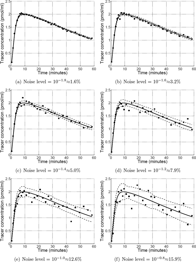
Computer simulations and analyses were performed in GNU Octave (Eaton 2002). Reference and target region data were simulated using a one-tissue compartment model with kinetics similar to moderate affinity receptor-ligand tracers such as [11C]raclopride and [11C]flumazenil. True binding potential in the target region was set equal to 2.0. Poisson-like noise (see Equation (9)) was added to the noiseless data to generate 500 pairs of target and reference region curves at each of 11 noise levels (1.6 to 16% fractional standard deviation at peak of target region curve) and 11 reference-to-target region volume ratios . Example time activity curves at different noise levels are show in Appendix C.
3.1.1. Comparison of weighting methods
The BFM and MRTM models were fit to the simulated data using a weighted least squares approach with either Standard or Reference weighting. As can be seen from Equation (10), the Reference weighting factors depend on the value of the model parameter R1. The Reference weights were therefore determined in two different ways. In one, the weights were determined with R1 fixed at one (true value = 1.2). The model was then applied in the usual fashion with R1 as an estimated parameter. In the other, the model was applied iteratively with the Reference weights updated based on the value of R1 estimated at the most recent iteration. The initial guess for R1 was one and convergence was determined using a relative tolerance of 10−3. As done previously (Ichise et al. 2003,Wu&Carson 2002), fits were considered outliers if the estimated value of either R1 or BPND was negative or greater than five times the true value. The comparisons performed in this study tested the hypothesis that the SRTM would perform better using Reference weighting factors than with Standard weights.
3.1.2. Comparison of reference regions
We considered a hypothetical region comprised of two kinetically distinct and separable tissue types: one that was an ideal reference tissue with no specific binding, and a non-ideal one having kinetics consistent with a receptor density equal to 10% of the target region. The reference region used to obtain the input function was either the ideal reference tissue alone or the sum of the ideal and non-ideal tissues. Thus, the first curve had ideal reference tissue kinetics, but was obtained from a smaller region and was therefore unbiased but noisy, whereas the second curve was biased but with better signal-to-noise. The BFM and MRTM models were fit to the data as described above, using Standard weighting with the input derived from the larger region or Reference weighting with the input function derived from the smaller region. The purpose of this comparison was to determine whether Reference weighting would justify the selection of smaller, more homogeneous reference regions.
3.2. Positron emission tomography studies
PET data were acquired dynamically from twenty-five healthy human subjects after injection of [11C]flumazenil, a central benzodiazepine receptor ligand. One group of seventeen subjects underwent single PET scans on an ECAT Exact HR+ scanner (Siemens Medical Systems, Knoxville, TN). One group of four subjects underwent two PET scans each on an ECAT Exact 47 camerai (Siemens Medical Systems, Knoxville, TN). Another group of four subjects underwent two PET scans each, once during a baseline condition and with a blocking dose of unlabeled flumazenil. Two of these subjects were scanned on the HR+ and two were scanned with the Exact-47. All data were acquired in 3D mode and binned into fifteen sinograms with the following time frames: 4 × 30 sec, 3 × 60 sec, 2 × 150 sec, 2 × 300 sec, 4 × 600 sec. Images were reconstructed with corrections for scatter, attenuation, dead-time, and detector non-uniformity using an ordered subset expectation maximization (OSEM) algorithm (four iterations, sixteen subsets) for data acquired on the HR+ or filtered backprojection (Hanning filter with 0.5 cutoff) for data acquired with the Exact-47. These studies were approved by the University of Michigan Institutional Review Board and all subjects provided informed consent.
Dynamic PET images were motion corrected and aligned to a sterotactic orientation using the NeuroStat image analysis software suite (Minoshima et al. 1993, Minoshima et al. 1994). Time activity curves were extracted from each of sixty-six regions of interest using a template based on the Talairach atlas. The BFM and MRTM models were applied to ROI data with Standard or Reference weights (calculated with R1 = 1) using the pons as a reference region. The in vivo kinetics of [11C]flumazenil are well-described by a one-tissue compartment model (Koeppe et al. 1991), so use of the SRTM is entirely justified.
Fractional differences between BPND values estimated with Standard or Reference weights were compared using the Wilcoxon matched-pairs signed-ranks test. The within-region variance of BPND estimated using either weighting scheme was determined across subjects in the baseline condition. We note that values of BPND are expected to vary not only between regions, but also between subjects for a given region. Hence the within-region measure of variance reflects intersubject variability as well as the intrinsic uncertainty of BPND estimates. On the other hand, the implicit parameter should theoretically be constant across regions within a given data set because there is only one reference region curve for each scan (Wu & Carson 2002, Ichise et al. 2003). For this reason, the within-scan variability of across regions was calculated as an alternative indicator of the precision of model parameters.
4. Results
4.1. Simulation study: Comparison of weighting methods
4.1.1. Reference weighting with R1 fixed
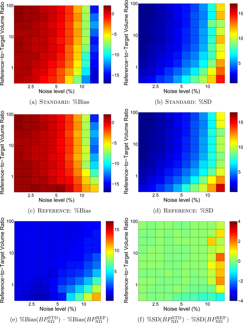
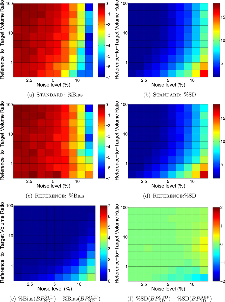
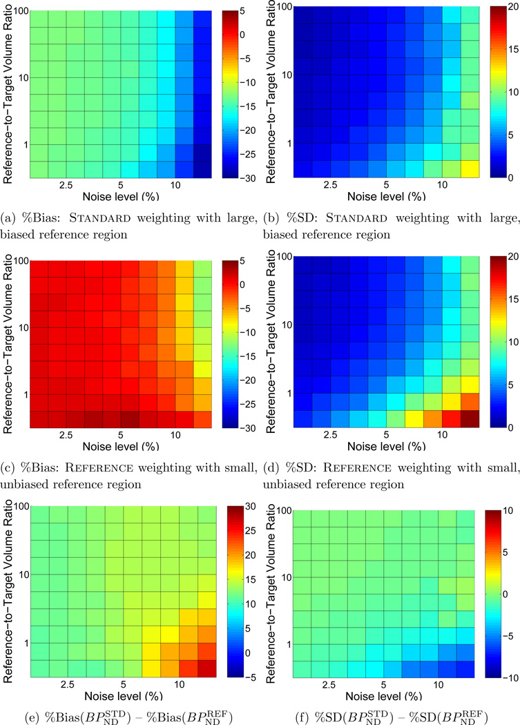
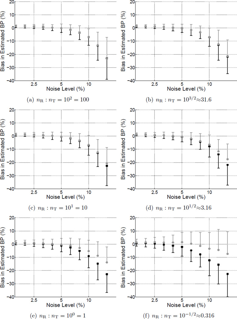
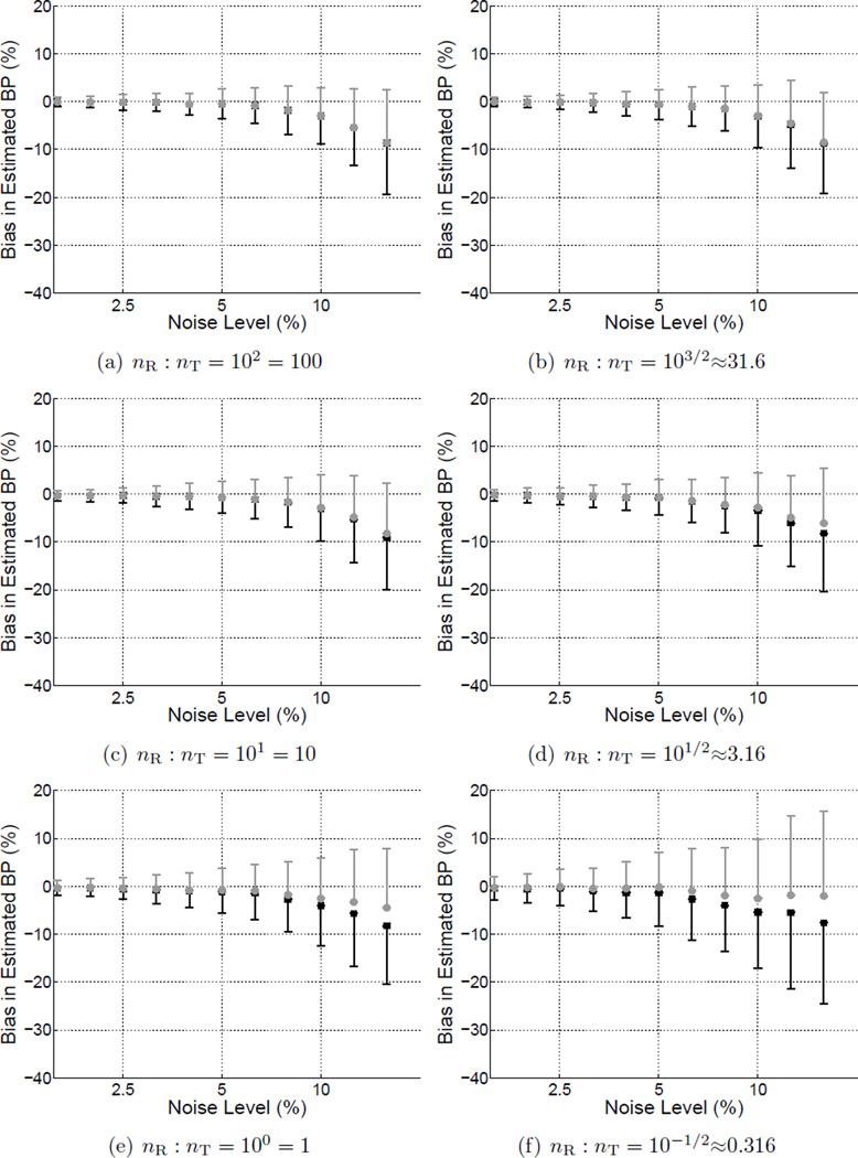
Figure 2 shows the bias (a,b) and precision (c,d) of BPND estimated by BFM with either Standard weighting or Reference weights calculated with R1 fixed. In each subplot the noise level increases moving toward the right and the size of the target region relative to the reference regions decreases moving toward the top. BPND was negatively biased and more variable at high noise levels for both weighting approaches. Reference weighting improved the accuracy (Figure 2(e)) and to a lesser extent the precision (Figure 2(f)) of estimated BPND as compared to Standard weighting, as shown in the difference maps of Figure 2(e,f) where positive values indicate lower bias and variance for results of the Reference weighting method. The advantage became more pronounced as noise increased and the relative size of the reference region decreased, reaching maximum effect at the highest noise level and when the reference tissue was smaller than the target region (lower right of each plot). There was little impact on performance with large reference regions or at low noise levels. Similarly, MRTM was more accurate (Figure 3(e)) with Reference than Standard weighting, although improvement in absolute precision was less pronouced (Figure 3(f)).
Figure 2.
Comparison of bias and standard deviation of BPND values estimated by BFM using Standard weighting or Reference with R1 fixed. In each subplot noise increases moving toward the right and the size of the target region relative to the reference region decreases moving toward the top. Bias and standard deviation are indicated by the color scale and expressed as percentages relative to the true value of BPND. (a), (c), and (e) each cover a range of 20 percentage points to facilitate comparisons. (b) and (d) are scaled alike, but (f) spans a smaller range (8 vs. 20 percentage points) to aid visualization. In the difference plots of (e) and (f), greater values indicate better performance by Reference than Standard weighting. Improvements in bias and precision were most pronounced at high noise levels and when the target and reference regions were of similar size. Figure C1 presents a subset of these results for selected region sizes as plots of bias ± s.d. as a function of noise level.
Figure 3.
Comparison of BPND estimated with Standard or Reference (R1 fixed) weighting using MRTM, presented as in Figure 1. (a), (c), and (e) share a common scale. (b) and (d) are scaled alike, but (f) spans a smaller range to aid visualization. Bias and standard deviation are expressed as percentages relative to the true value of BPND. Figure C2 presents a subset of these results for selected region sizes as plots of bias ± s.d. as a function of noise level.
4.1.2. Reference weighting with R1 updated iteratively
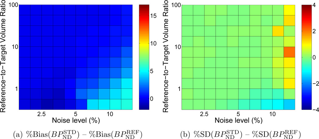
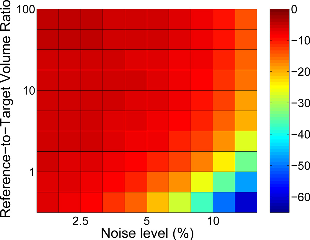
Similar to Reference weighting using a value for fixed R1, the bias and variability of BPND were smaller using Reference weighting with R1 iterated than using Standard weighting. The greatest reductions in bias and variability occurred when noise was high and the target and reference regions were of similar size (Figure 4), where greater values indicate improved performance with Reference weighting. Comparing these results to those shown in analogous difference plots of Figure 2(e,f) indicates that Reference weighting improved accuracy more when factors were calculated with R1 fixed than with R1 iterated (note that the scales of Figure 2(e) and Figure 4(e) are identical). The precision was similar for either variant of Reference weighting. Trends were comparable for MRTM (not shown). R1 was increasingly underestimated as noise increased and as the volume of the reference region decreased (Figure 5).
Figure 4.
Comparison of accuracy and precision in BPND estimated by BFM using Standard weighting or Reference weighting with R1 updated iteratively. Difference plots for (a) bias and (b) standard deviation are presented as in Figure 2(e,f), where greater values indicate lower bias and better precision with the Reference weighting method. Comparing (a) and (b) directly to Figure 2(e,f) (note the matching scales) indicates that the performance of Reference with R1 iterated was intermediate between Standard and Reference with R1 fixed. Results with MRTM were similar.
Figure 5.
Bias in R1 using Reference with R1 updated iteratively. Underestimation of R1 de-emphasizes the contribution of the reference region to the calculated variance of residuals (see Equation (10)). Thus, the performance of Reference with R1 iterated was intermediate between Standard weighting and Reference with R1 fixed (Figures 2(e,f), 4(a,b)).
4.2. Simulation study: Comparison of reference regions
Even at low noise levels, negative bias in BPND estimated with BFM was considerable (~14%, see Figure 6(a)) when data from the large, heterogeneous reference region was used as the input function with Standard weighting. In contrast, the smaller (but kinetically ideal) tissue with Reference weighting yielded essentially unbiased estimates of BPND at low noise (Figure 6(a)). BPND values obtained using Reference with the smaller region were less biased than those estimated using Standard with the larger region for all combinations of noise level and region size (Figure 6(e)). As expected, absolute precision was better for Standard with a large reference region, consistent with the higher signal-to-noise ratio of the input data. However, in terms of the coefficient of variation of variation of BPND, the precision obtained using the small region with Reference weighting is comparable to that of the large region with Standard weighting, whereas the accuracy is better across all combinations of noise levels and region sizes.
Figure 6.
Comparison of accuracy and precision of BPND estimated by BFM using Standard weighting with a large, heterogeneous reference tissue biased by the presence of specific binding or Reference weighting (R1 fixed) with small, ideal reference region. BPND values obtained with Standard weighting and biased input data were underestimated by 14% or more across all noise levels and region sizes, whereas values estimated with Reference weighting were essentially unbiased except at high very noise levels. Absolute variance was greater with Reference weighting, but the coefficient of variation was comparable to Standard. Bias and standard deviation are expressed as percentages relative to the true value of BPND.
4.3. Human imaging studies
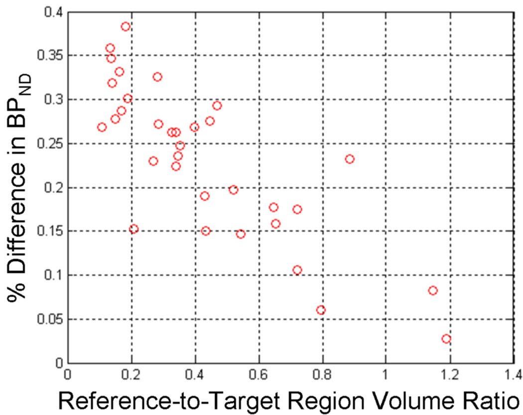
BPND estimates obtained using Reference weighting were greater than values estimated using Standard weights for 1651 of 2177 curves (75.8%) via BFM and 1786 of 2176 (82.1%) data sets via MRTM. Of the 2178 analyzed target region curves (33 scans × 66 regions per scan), one data set yielded negative BPND values with MRTM using both Standard and Reference weighting and was excluded from statistical analysis. One additional data set yielded unphysiological BPND values when analyzed by MRTM and was also excluded. The average increase in BPND with Reference weighting was small (0.38%±0.53% for BFM, 0.23%±0.31% for MRTM) but highly significant (p < 10−10, Wilcoxon matched-pairs signed-ranks). Increases in BPND attributable to Reference weighting were greater for data sets acquired on the HR+ and reconstructed with OSEM (0.41%±0.15% for BFM, 0.25%±0.10% for MRTM) than those acquired on the Exact-47 with FBP reconstruction (0.33%±0.17% for BFM, 0.22%±0.09% for MRTM). No differences in the precision of BPND were observed between weighting approaches. Estimates of from either weighting method showed no substantial difference in absolute values (across subjects, 0.31±0.07 vs. 0.30±0.07 min−1 with BFM and 0.28±0.05 vs. 0.27±0.05 min−1 with MRTM) or variability (within-subject fractional standard deviation equal 16.2±6.5 vs. 16.6±6.9% for BFM and 15.5±5.5 vs. 16.2±0.05% for MRTM). For both BFM and MRTM, an inverse relationship was observed for the fractional difference in BPND between Reference and Standard weighting (i.e., the magnitude of Reference weighting’s effect) and the volume of the reference region relative to the target region (Figure 7), consistent with the findings of the simulation studies.
Figure 7.
Percent increase in BPND estimated from human [11C]flumazenil data using Reference compared to Standard weighting as a function of relative region size. Fractional change was averaged across all 33 scans for each of the 33 uniquely sized brain regions. The trend toward greater effect of Reference weighting for larger target region volumes is consistent with findings of the simulation studies. The linear regression fit was y = −0.25x+0.34 and, though not strictly valid over a wider range region sizes, adequately described the relationship with a correlation coefficient of r = 0.69.
5. Discussion
We have demonstrated that accounting for noise in the input function when choosing weighting factors can improve the quantitation of binding potential with two common formulations of the simplified reference tissue model. Our first simulation study indicated that the greatest improvement in performance occurred at high noise levels and when the the target and reference regions were of similar size (Figures 2,4). Analysis of region-of-interest data from [11C]flumazenil experiments in humans using the pons as the reference tissue showed a small but highly significant increase in BPND using Reference as compared to Standard weighting. These results support the findings of our simulation study and demonstrate a statistical impact of Reference weighting on clinical data. However, the magnitude of the observed increase in BPND suggests that Reference weighting alone has a marginal effect at noise levels typically encountered in ROI-based analyses of human PET data. Thus, we posit that Reference weighting may be most beneficial for small animal imaging, when noise level varies between data sets (due to differences in injected radioactivity, for example), or any time the statistical properties of the input function are especially poor. Similarly, this technique may be particularly useful when the amount of radioactivity must be limited for pharmacological reasons (e.g., with agonist tracers, high affinity ligands, or radiosyntheses yielding low specific activity) or to minimize radiation exposure.
A trend toward greater effect of Reference weighting with larger target regions was observed in the [11C]flumazenil data (Figure 7), also consistent with simulation results. We note that the size of the reference tissue was fixed, whereas target regions of different volumes were analyzed. In contrast to simulation studies where we were able to manipulate region volume and noise level independently, for these experimental data the size of the target region influenced not only the relative volumes of the reference and target regions (the vertical position of the operating point in Figures 2 to 6, with smaller target regions appearing nearer the top) but also the noise level of the target region data (the horizontal position, with noisier curves towards the right). In particular, according to the Poisson-like noise model we expect that an n-fold change in target region volume will yield a -fold reduction in noise level. Given the topologies observed in Figures 2 to 6, we cannot exclude the possibility that the [11C]flumazenil curves generated from target regions of different sizes fell approximately along an isocontour, diminishing the relationship between impact of weighting method and relative region size.
The second of our simulation experiments indicated that analyses carried out with a smaller, unbiased reference tissue coupled with Reference weighting were more accurate than those using a larger, non-ideal reference region with Standard weighting, as is often done in practice to reduce noise in the input function. In terms of absolute precision (e.g., relative to the true parameter value), the estimates of BPND obtained with the larger reference region were less variable, consistent with the lower noise of that input curve. However, if variability is considered relative to the estimated parameter values (i.e., the coefficient of variation), the two approaches have similar precision. Therefore, both methods should have similar ability to differentiate populations, while the use of a smaller reference region with Reference weighting would offer the advantage of reduced bias for quantitative applications which benefit from accurate estimates of BPND and unbiased reference region data. The use of a smaller, more appropriate reference region could be envisioned when putative reference tissues are heterogeneous with subregions having specific binding or non-specific binding inconsistent with target tissues, or when the conventional reference region is susceptible to signal contamination from adjacent tissues (i.e., spillover due to partial volume effects).
5.1. Iteration of R1
The model parameter R1 appears in the Reference approximation of uncertainty in the residuals (Equation (10)). We therefore considered two alternative approaches, either assigning the weights with R1 fixed at an assumed (and in these simulations, incorrect) value of one or fitting the data iteratively and updating the weights using the value of R1 estimated at the previous iteration. We hypothesized that using the estimated R1 would more accurately apportion the respective contributions of the target and reference region data to the total uncertainty of the residuals and thereby provide better results, but were initially surprised to find that the performance of Reference with R1 iterated was intermediate between Standard and Reference weighting with R1 fixed. This result can be explained by the severe underestimation of R1 at high noise levels (Figure 5). Note that the Reference weights given by Equation (10) tend toward the Standard weights given by Equation (9) as R1 decreases, consistent with the intermediate performance of the Reference method when weighting factors were selected using the estimated value of R1 (Figure 4). Parameter bounds or constraints may improve the stability of the method in the presence of noise, but in the current formulation we recommend fixing R1 when calculating Reference weighting factors.
5.2. Choice of noise model
In this work we have assumed that the uncertainty of the PET image data can be represented by Poisson-like distributions. Although Poisson statistics are strictly valid only at the event level, this approximation is employed frequently to model noise in the image domain for PET data analysis (e.g., (Landaw & DiStefano 1984, Mazoyer et al. 1986, Jovkar et al. 1989, Delforge et al. 1990, Chen et al. 1991, Feng et al. 1991, Vera et al. 1992, Millet et al. 1996)). Alternative error approximations derived by empirical (Budinger et al. 1978, Watabe et al. 2000, Buvat 2002) and analytical (Alpert et al. 1982, Huesman 1984, Defrise et al. 1990, Carson et al. 1993, Pajevic et al. 1998, Qi 2003) procedures have been proposed and the development of more accurate models continues to be an active area of research. The most appropriate noise model is generally considered to be dependent on the acquisition type (2D vs. 3D), reconstruction algorithm (e.g., filtered backprojection vs. expectation maximization), and other physical factors such as voxel size, system resolution, and detector design. It is not our intent in this paper to endorse the merits or generality of any particular noise model, and we note that the framework for Reference weighting described in this manuscript is generic and can be readily modified to accommodate whatever noise model is deemed most appropriate for the data at hand.
In implementing the Poisson noise model we have calculated the variance based on the noisy data. This approach assumes that the PET measurement is a reasonable approximation of the true radioactivity concentration. This estimate is asymptotically correct for low noise levels, but its validity diminishes as noise increases. For this reason, it would be preferable to use iteratively reweighted least squares or another technique that derives the weighting factors from the model fit rather than the measured data, particularly with noisier data (Spilker & Vicini 2001, Muzic & Christian 2006). Such approaches cannot be applied directly to the Reference weighting method because the SRTM provides a model fit to the target region data, but not to the reference region input function. Methods to obtain fits to both regions simultaneously are under investigation.
5.3. Assumptions and simplifications
We have made several assumptions that simplify the Reference method and improve its practical utility. The secondary terms in the BFM and MRTM operational equations were assumed to be effectively noiseless because integration effectively smooths noisy data (Ichise et al. 2002). The noise in the target and reference region data was assumed to be uncorrelated. This approximation relies on the regions being sufficiently separated in space and the data being free of systemic error from reconstruction or motion artifacts. Finally, the error approximations were obtained from reconstructed image data only, in contrast with the method of Huesman and Mazoyer (Huesman & Mazoyer 1987) which was applied at the sinogram level to determine the variance of the PET data (Huesman 1984). While this approach is effective and elegant, the need to operate on sinograms, and in particular, to define regions of interest in sinogram space, renders the method cumbersome in practice (Carson et al. 1993). We believe that approximating the noise from the image data represents a reasonable tradeoff between accuracy and ease of use. As with the choice of noise model, the Reference weighting approach can be easily adapted if any of these simplifications are found to be invalid: the expression for the variance of the residuals could account for correlated noise or uncertain secondary terms in the operational equation by including the covariance or integral terms, and image-derived error approximations could be replaced with formulas that make use of sinogram data or other noise models, as described above.
6. Conclusions
The Reference weighting approach accounts for the statistical uncertainty of the reference region input function during selection of weighting factors. Simulation studies verified that Reference weighting improves SRTM performance at higher noise levels and when the target and reference regions are of comparable size. Region-based analysis of [11C]flumazenil data from humans showed a small but significant increase in binding potential estimates when Reference weights were used and that the magnitude of the effect is associated with the relative sizes of the target and reference regions, consistent with the results of our simulation study. We have also shown with simulations that quantification of BPND may be improved by using a smaller, more appropriate reference tissue in tandem with Reference weighting. These results suggest that Reference weighting may be useful for small animal imaging, when injected radioactivity is limited by mass dose of tracer, or when a smaller reference tissue could be selected to avoid bias introduced by specific binding or partial volume effects. These benefits of Reference weighting may also apply to other models derived from the SRTM or to reference region methods, generally.
Figure B1.
Simulated time activity curves over a range of noise levels. Markers depict a representative noisy time activity curve. Solid curve shows the noiseless time activity curve. Dashed curves form an envelope of one standard deviation about the mean at each time point across 500 noise replicates.
Figure C1.
Bias of BPND as a function of noise level for estimates obtained using BFM with Reference (gray markers) or Standard weighting (black markers). Error bars represent the standard deviation across simulated data sets. The subplots each correspond to a different reference-to-target region volume ratio and collectively depict an alternative way to visualize a subset of the results presented in Figure 2.
Figure C2.
Bias of BPND as a function of noise level for estimates obtained using MRTM with Reference (gray markers) or Standard weighting (black markers). Error bars represent the standard deviation across simulated data sets. The subplots each correspond to a different reference-to-target region volume ratio and collectively depict an alternative way to visualize a subset of the results presented in Figure 3.
Acknowledgments
The authors acknowledge the support of the Society of Nuclear Medicine Student Fellowship Award to M.D. Normandin and NIH grant R21 AA015077 to E.D. Morris.
Appendix A
Derivation of Reference weighting
Assuming Poisson-like statistics, the variance of PET image data in a region of interest can be approximated by Equation (9). Hence the variances of the target and reference region radioactivity data at the ith frame of the dynamic PET series are given by
| (A.1) |
and
| (A.2) |
where C is the measured tracer concentration and the subscripts T and R refer to the target and reference regions.
The residuals, ri, are defined as the difference between the measured target region data, di, and the model predicted values, mi:
| (A.3) |
A general expression for the variance of the residuals is given by
| (A.4) |
For our purposes, di corresponds to the measured target region PET data, CT(ti), and mi is given by the output of the BFM or MRTM operational equations shown in Equations (7) and (8), respectively. Note that the basis functions of Equation (7) contains a convolution term and Equation (8) has two running integrals. Convolution smooths the data and integration sums it, both of which act as noise-reducing operators. We therefore regard the convolution and integral terms as effectively noiseless, and so Equation (A.4) can be simplified to
| (A.5) |
If we further assume that the statistical uncertainties of the target and reference region data are uncorrelated, the covariance term vanishes and the expression simplifies to
| (A.6) |
Substituting Equations (A.1) and (A.2) into Equation (A.6) yields the expression for the variance of each residual as
| (A.7) |
If the scaling factor ζ is constant (specifically, the same in the target and reference regions), we can let ζT = ζR = ζ and Eq (A.7) simplifies to
| (A.8) |
which is identical to Equation (10), the expression used to calculate the Reference weighting factors.
Appendix B
Example time activity curves for different noise levels
Appendix C
Alternative plots of performance as a function of noise level
Figures plotting bias±s.d. as a function of noise level at selected regions are shown as an alternative way to view a subset of the results presented in Figures 2 and 3.
References
- Alpert NM, Badgaiyan RD, Livni E, Fischman AJ. NeuroImage. 2003;19(3):1049–1060. doi: 10.1016/s1053-8119(03)00186-1. [DOI] [PubMed] [Google Scholar]
- Alpert NM, Chesler DA, Correia JA, Ackerman RH, Chang JY, Finklestein S, Davis SM, Brownell GL, Taveras JM. IEEE Trans Med Imaging. 1982;1(2):142–146. doi: 10.1109/TMI.1982.4307561. [DOI] [PubMed] [Google Scholar]
- Aston JA, Gunn RN, Worsley KJ, Ma Y, Evans AC, Dagher A. NeuroImage. 2000;12(3):245–256. doi: 10.1006/nimg.2000.0620. [DOI] [PubMed] [Google Scholar]
- Blomqvist G, Pauli S, Farde L, Eriksson L, Persson A, Halldin C. Eur J Nucl Med. 1990;16(4–6):257–265. doi: 10.1007/BF00842777. [DOI] [PubMed] [Google Scholar]
- Budinger TF, Derenzo SE, Greenberg WL, Gullberg GT, Huesman RH. J Nucl Med. 1978;19(3):309–315. [PubMed] [Google Scholar]
- Buvat I. Phys Med Biol. 2002;47(10):1761–1775. doi: 10.1088/0031-9155/47/10/311. [DOI] [PubMed] [Google Scholar]
- Carson RE, Yan Y, Daube-Witherspoon ME, Freedman N, Bacharach SL, Herscovitch P. IEEE Trans Med Imaging. 1993;12(2):240–250. doi: 10.1109/42.232252. [DOI] [PubMed] [Google Scholar]
- Chen KW, Huang SC, Yu DC. Phys Med Biol. 1991;36(9):1183–1200. doi: 10.1088/0031-9155/36/9/003. [DOI] [PubMed] [Google Scholar]
- Chiao PC, Rogers WL, Clinthorne NH, Fessler JA, Hero A. IEEE Transactions on Medical Imaging. 1994;13(2):217–226. doi: 10.1109/42.293914. [DOI] [PubMed] [Google Scholar]
- Cunningham VJ, Hume SP, Price GR, Ahier RG, Cremer JE, Jones AK. J Cereb Blood Flow Metab. 1991;11(1):1–9. doi: 10.1038/jcbfm.1991.1. [DOI] [PubMed] [Google Scholar]
- Defrise M, Townsend D, Deconinck F. Phys. Med. Biol. 1990;35(1):131–138. doi: 10.1088/0031-9155/35/10/002. [DOI] [PubMed] [Google Scholar]
- Delforge J, Syrota A, Mazoyer BM. IEEE Trans Biomed Eng. 1990;37(7):653–661. doi: 10.1109/10.55673. [DOI] [PubMed] [Google Scholar]
- Eaton JW. GNU Octave Manual. Network: Theory Limited; 2002. [Google Scholar]
- Feng D, Wang X, Fulton R, Hutton B, Morris J. Biomed Sci Instrum. 1991;27:43–48. [PubMed] [Google Scholar]
- Gunn RN, Lammertsma AA, Hume SP, Cunningham VJ. NeuroImage. 1997;6(4):279–287. doi: 10.1006/nimg.1997.0303. [DOI] [PubMed] [Google Scholar]
- Huesman RH. Phys Med Biol. 1984;29(5):543–552. doi: 10.1088/0031-9155/29/5/007. [DOI] [PubMed] [Google Scholar]
- Huesman RH. Phys Med Biol. 1997;42(1):147–153. doi: 10.1088/0031-9155/42/1/010. [DOI] [PubMed] [Google Scholar]
- Huesman RH, Mazoyer BM. Phys Med Biol. 1987;32(12):1569–1579. doi: 10.1088/0031-9155/32/12/004. [DOI] [PubMed] [Google Scholar]
- Ichise M, Cohen RM, Carson RE. J Cereb Blood Flow Metab. 2008;28(2):420–430. doi: 10.1038/sj.jcbfm.9600530. [DOI] [PubMed] [Google Scholar]
- Ichise M, Liow JS, Lu JQ, Takano A, Model K, Toyama H, Suhara T, Suzuki K, Innis RB, Carson RE. J Cereb Blood Flow Metab. 2003;23(9):1096–1112. doi: 10.1097/01.WCB.0000085441.37552.CA. [DOI] [PubMed] [Google Scholar]
- Ichise M, Toyama H, Innis RB, Carson RE. J Cereb Blood Flow Metab. 2002;22(10):1271–1281. doi: 10.1097/01.WCB.0000038000.34930.4E. [DOI] [PubMed] [Google Scholar]
- Ikoma Y, Watabe H, Hayashi T, Miyake Y, Teramoto N, Minato K, Iida H. NeuroImage. 2009;47(4):1639–1648. doi: 10.1016/j.neuroimage.2009.05.099. [DOI] [PubMed] [Google Scholar]
- Innis RB, Cunningham VJ, Delforge J, Fujita M, Gjedde A, Gunn RN, Holden J, Houle S, Huang SC, Ichise M, Iida H, Ito H, Kimura Y, Koeppe RA, Knudsen GM, Knuuti J, Lammertsma AA, Laruelle M, Logan J, Maguire RP, Mintun MA, Morris ED, Parsey R, Price JC, Slifstein M, Sossi V, Suhara T, Votaw JR, Wong DF, Carson RE. J Cereb Blood Flow Metab. 2007;27(9):1533–1539. doi: 10.1038/sj.jcbfm.9600493. [DOI] [PubMed] [Google Scholar]
- Jovkar S, Evans AC, Diksic M, Nakai H, Yamamoto YL. Phys Med Biol. 1989;34(7):895–908. doi: 10.1088/0031-9155/34/7/010. [DOI] [PubMed] [Google Scholar]
- Koeppe RA, Holthoff VA, Frey KA, Kilbourn MR, Kuhl DE. J Cereb Blood Flow Metab. 1991;11(5):735–744. doi: 10.1038/jcbfm.1991.130. [DOI] [PubMed] [Google Scholar]
- Lammertsma AA, Hume SP. NeuroImage. 1996;4(3 Pt 1):153–158. doi: 10.1006/nimg.1996.0066. [DOI] [PubMed] [Google Scholar]
- Landaw EM, DiStefano JJ., 3rd Am J Physiol. 1984;246(5 Pt 2):R665–R677. doi: 10.1152/ajpregu.1984.246.5.R665. [DOI] [PubMed] [Google Scholar]
- Mazoyer BM, Huesman RH, Budinger TF, Knittel BL. J Comput Assist Tomogr. 1986;10(4):645–653. doi: 10.1097/00004728-198607000-00020. [DOI] [PubMed] [Google Scholar]
- Millet P, Delforge J, Pappata S, Syrota A, Cinotti L. Phys Med Biol. 1996;41(12):2739–2756. doi: 10.1088/0031-9155/41/12/012. [DOI] [PubMed] [Google Scholar]
- Minoshima S, Koeppe RA, Frey KA, Kuhl DE. Journal of Nuclear Medicine. 1994;35(9):1528–1537. [PubMed] [Google Scholar]
- Minoshima S, Koeppe RA, Mintun MA, Berger KL, Taylor SF, Frey KA, Kuhl DE. Journal of Nuclear Medicine. 1993;34(2):322–329. [PubMed] [Google Scholar]
- Mintun MA, Raichle ME, Kilbourn MR, Wooten GF, Welch MJ. Ann Neurol. 1984;15(3):217–227. doi: 10.1002/ana.410150302. [DOI] [PubMed] [Google Scholar]
- Møller M, Rodell A, Gjedde A. Journal of Nuclear Medicine. 2009;50:1229–1236. doi: 10.2967/jnumed.108.053322. [DOI] [PubMed] [Google Scholar]
- Muzic RF, Jr, Christian BT. Med Phys. 2006;33(2):342–353. doi: 10.1118/1.2135907. [DOI] [PubMed] [Google Scholar]
- Normandin MD, Schiffer WK, Morris ED. NeuroImage. in press. [Google Scholar]
- Pajevic S, Daube-Witherspoon ME, Bacharach SL, Carson RE. IEEE Trans Med Imaging. 1998;17(1):9–23. doi: 10.1109/42.668691. [DOI] [PubMed] [Google Scholar]
- Qi J. Phys Med Biol. 2003;48(21):3505–3519. doi: 10.1088/0031-9155/48/21/004. [DOI] [PubMed] [Google Scholar]
- Snyder DL. IEEE Trans Biomed Eng. 1973;20(1):11–20. doi: 10.1109/TBME.1973.324246. [DOI] [PubMed] [Google Scholar]
- Spilker ME, Vicini P. J Biomed Inform. 2001;34(5):348–364. doi: 10.1006/jbin.2001.1033. [DOI] [PubMed] [Google Scholar]
- Thiele F, Buchert R. Nucl Med Commun. 2008;29(2):179–188. doi: 10.1097/MNM.0b013e3282f28138. [DOI] [PubMed] [Google Scholar]
- Tomasi G, Bertoldo A, Schmidt K, Turkheimer F, Smith C, Cobelli C. NeuroImage. 2008a;41(S2):T84. [Google Scholar]
- Tomasi G, Edison P, Bertoldo A, Roncaroli F, Singh P, Gerhard A, Cobelli C, Brooks DJ, Turkheimer F. J Nucl Med. 2008b;49(8):1249–1256. doi: 10.2967/jnumed.108.050583. [DOI] [PubMed] [Google Scholar]
- Vera DR, Scheibe PO, Krohn KA, Trudeau WL, Stadalnik RC. IEEE Trans Biomed Eng. 1992;39(4):356–367. doi: 10.1109/10.126608. [DOI] [PubMed] [Google Scholar]
- Watabe H, Endres CJ, Breier A, Schmall B, Eckelman WC, Carson RE. J NuclMed. 2000;41(3):522–530. [PubMed] [Google Scholar]
- Wu Y, Carson RE. J Cereb Blood Flow Metab. 2002;22(12):1440–1452. doi: 10.1097/01.WCB.0000033967.83623.34. [DOI] [PubMed] [Google Scholar]
- Zhou Y, Chen MK, Endres CJ, Ye W, Brasic JR, Alexander M, Crabb AH, Guilarte TR, Wong DF. NeuroImage. 2006;33(2):550–563. doi: 10.1016/j.neuroimage.2006.06.038. [DOI] [PubMed] [Google Scholar]
- Zhou Y, Endres CJ, Brasic JR, Huang SC, Wong DF. NeuroImage. 2003;18(4):975–989. doi: 10.1016/s1053-8119(03)00017-x. [DOI] [PubMed] [Google Scholar]


