Optimization of the algorithms for estimating the ultrasonic attenuation along the propagation path

Abstract

In this study, we perform statistical analysis on two methods used to estimate the total ultrasound attenuation along the propagation path from the surface of the transducer to a region of interest at a particular depth; namely, the spectral-fit method and the multiple-filter method. We derive mathematical equations for the bias and variance in the attenuation estimates as a function of region of interest (ROI) size, imaging system bandwidth, and number of independent Gaussian filters (for the multiple filter method). We use numerical simulations to validate the mathematical equations and compare the two algorithms. The results show that the variance in the total attenuation coefficient estimates obtained with the two methods are comparable, and that the estimates are unbiased. For the multiple filter method, the optimal number of Gaussian filters is two.

I. INTRODUCTION

Knowing the total ultrasonic attenuation along the propagation path from the transducer surface to the ROI in the sample is essential in many medical ultrasound applications. In the area of ultrasonic tissue characterization, accurate estimates of the scatterer size and the backscatter coefficient can only be obtained if the total attenuation is known [1–3]. In ultrasound therapy applications, the total attenuation is used to calculate the intensity of ultrasound that reaches the region of interest (ROI) and hence quantify the amount of heating that is produced [4, 5]. In ultrasonic imaging, time gain compensation can be done more accurately if the total attenuation is known, and therefore eliminate shadowing and enhancement regions in the image [6]. In acoustic radiation force imaging, the total attenuation is used to quantify the amount of radiation force applied to the ROI [7, 8]. Therefore many areas of clinical medical ultrasound would benefit from an accurate estimate of the total attenuation along the propagation path.

Traditionally, the total attenuation was estimated by measuring changes in the backscatter intensity with depth [9, 10]. However, this method is inaccurate because the attenuation, the backscatter, and the diffraction effects modify the power spectrum of the backscattered radio frequency (RF) signals. Some investigators estimated the local attenuation coefficients and the thicknesses of the overlying tissues along the propagation path and then performed a weighted sum of these estimates to calculate the total attenuation [11]. Others assigned an attenuation coefficient value to each overlying tissue based on existing values that were measured ex-vivo [12]. These methods, however, are prone to error accumulation with propagation depth due to the inaccuracies in the thickness measurements (sound speed changes), the inaccuracies of the assigned attenuation coefficients which were measured ex-vivo (low blood perfusion), and the variability of the attenuation coefficients due to inter-patient variability. Furthermore, they require the identification of the different overlying tissues, a process that may require manual intervention.

Recently, two methods for estimating the total attenuation have been developed; namely, the spectral-fit method and the multiple-filter method [13–16]. Both methods use a planar reflector to compensate for the effects of diffraction, the transducer transfer function, and the transmit-pulse transfer function. The first approach, named the spectral-fit algorithm, assumes a Gaussian Form Factor and estimates the total attenuation and the scatterer size simultaneously [16]. The second approach, named the multiple-filter algorithm estimates the total attenuation by processing the spectra that result from multiplying the backscatter power spectrum by Gaussian filters [13–15]. In a recent paper by Labyed et al [17], the multiple filter method was modified by employing a tissue-mimicking phantom (TMP) instead of a planar reflector to compensate for the transfer function of the transducer and the diffraction effects that result from focusing. Using a tissue-mimicking reference phantom makes the algorithm practical for use in clinical settings where beam-formed echoes are obtained from array sources.

The objective of this study is to test and compare the accuracies of the spectral-fit method and the multiple-filter method. We perform statistical analysis and derive mathematical equations for the expected value and the variance of the attenuation estimates as a function of transducer bandwidth, ROI size (the region where backscattered echoes are acquired to retrieve estimates of the attenuation), and number of independent Gaussian filters (for the multiple-filter method). We then use numerical simulation to validate the derived equations and compare the two algorithms.”

II. Overview of the spectral-fit method and the multiple-filter method

A. Spectral-fit method

To estimate the total ultrasonic attenuation from the surface of the transducer to an ROI in a sample material, the same transducer and power settings are used to obtain backscattered signals from the sample, and from a reference TMP. The TMP has a known attenuation coefficient, and a propagation sound speed that closely matches the sound speed in soft tissue. The RF echo lines are windowed in order to obtain multiple adjacent time-gated windows corresponding to the ROI. The Fourier Transform is applied to every window, and the power spectra of the windows are averaged. The same procedure is performed on the region of the reference phantom that has the same depth compared to the ROI of the sample. In standard pulse-echo imaging, the power spectrum of a windowed region in a statistically homogeneous tissue is given by [1]

$$S_s(f,d)\propto H(f,d)F_s(f)\text{exp}(-4{\alpha }_s\mathit{\text{df}}).$$ (1)

The subscript s denotes the sample. The letter d denotes the distance from the surface of the transducer to the depth corresponding to the center of the time-gated window. The transfer function of the imaging system is given by H(f, d). The frequency-dependent scattering properties of the ROI are given by F_s(f). The attenuation along the propagation path is assumed linearly dependent on frequency and the attenuation coefficient slope is α_s. Equation (1) assumes that the windows used to gate the echoes are small compared to the depth of focus of the transducer so that the variations of the field within each gated region could be ignored [18]. Similarly, the power spectrum of the backscattered signal from the reference phantom is

$$S_r(f,d)\propto H(f,d)F_r(f)\text{exp}(-4{\alpha }_r\mathit{\text{df}}).$$ (2)

The subscript r denotes the reference phantom. Dividing the power spectrum of the sample by the power spectrum of the reference phantom yields

$$S(f)=\frac{S_s(f)}{S_r(f)}\propto \frac{F_s(f)}{F_r(f)}\times \text{exp}(-4\mathit{\text{df}}\mathrm{\Delta }\alpha )$$ (3)

where

$$\mathrm{\Delta }\alpha =({\alpha }_s-{\alpha }_r).$$ (4)

Insana showed that under the born approximation (weak scattering), the scattering terms can be written as [19, 20]

$$F_s(f)\propto f^4{F}_{\gamma s}(f,a_{\mathit{\text{eff}}\_s})$$ (5)

$$F_r(f)\propto f^4{F}_{\gamma r}(f,a_{\mathit{\text{eff}}\_r}),$$ (6)

where F_γs(f, a_{eff_s}) and F_γs(f, a_{eff_r}) are the form factors of the sample and the reference, respectively. The Form Factor is the ratio of the backscatter coefficient for a test material having scatterers with finite size to that of a similar material consisting of point scatterers [19]. a_{eff_s} and a_{eff_r} are the effective scatterer sizes of sub-resolution scatterers within the sample and the reference, respectively. If the form factors of both the sample and the reference are approximated by Gaussian Form Factors, we obtain

$$\begin{array}{c}{F}_s(f,a_{\mathit{\text{eff}}\_s})\propto \text{exp}(-B_s{f}^2)\hfill \\ F_r(f,a_{\mathit{\text{eff}}\_r})\propto \text{exp}(-B_r{f}^2),\hfill \end{array}$$ (7)

where B is proportional to the correlation length. Equation (3) becomes

$$\begin{array}{c}S(f)=\frac{S_s}{S_r}\propto \frac{\text{exp}(-B_s{f}^2)}{\text{exp}(-B_r{f}^2)}\text{exp}(-4\mathit{\text{df}}\mathrm{\Delta }\alpha )\hfill \\ \hfill S(f)\propto \text{exp}(-\mathrm{\Delta }{\mathit{\text{Bf}}}^2)\text{exp}(-4\mathit{\text{df}}\mathrm{\Delta }\alpha ),\hfill \end{array}$$ (8)

where ΔB = B_s − B_r. By taking the natural algorithm of Eq. (8), we obtain

$$S_{\text{ln}}(f)=\text{ln}[S(f)]=-\mathrm{\Delta }{\mathit{\text{Bf}}}^2-4\mathit{\text{df}}\mathrm{\Delta }\alpha +c.$$ (9)

Equation (9) is linear with respect to the unknown Δα. Therefore, Δα can be estimated using least linear squares [21]

$$\mathrm{\Delta }\alpha =\frac{L}{\mathrm{\Delta }}[{\displaystyle \sum _{i=1}^L}{f}_i{S}_{\text{ln}}(f_i){\displaystyle \sum _{i=1}^L}{f}_i^4-{\displaystyle \sum _{i=1}^L}{f}_i^3{\displaystyle \sum _{i=1}^L}{f}_i^2{S}_{\text{ln}}(f_i)]-\frac{{\displaystyle {\sum }_{i=1}^L}{S}_{\text{ln}}(f_i)}{\mathrm{\Delta }}[{\displaystyle \sum _{i=1}^L}{f}_i{\displaystyle \sum _{i=1}^L}{f}_i^4-{\displaystyle \sum _{i=1}^L}{f}_i^3{\displaystyle \sum _{i=1}^L}{f}_i^2]+\frac{{\displaystyle {\sum }_{i=1}^L}{f}_i^2}{\mathrm{\Delta }}[{\displaystyle \sum _{i=1}^L}{f}_i{\displaystyle \sum _{i=1}^L}{f}_i^2{S}_{\text{ln}}(f_i)-{\displaystyle \sum _{i=1}^L}{f}_i{S}_{\text{ln}}(f_i){\displaystyle \sum _{i=1}^L}{f}_i^2].$$ (10)

where

$$\mathrm{\Delta }=L[{\displaystyle \sum _{i=1}^L}{f}_i^2{\displaystyle \sum _{i=1}^L}{f}_i^4-{\left({\displaystyle \sum _{i=1}^L}{f}_i^3\right)}^2]-{\displaystyle \sum _{i=1}^L}{f}_i[{\displaystyle \sum _{i=1}^L}{f}_i{\displaystyle \sum _{i=1}^L}{f}_i^4-{\displaystyle \sum _{i=1}^L}{f}_i^3{\displaystyle \sum _{i=1}^L}{f}_i^2]+{\displaystyle \sum _{i=1}^L}{f}_i^2[{\displaystyle \sum _{i=1}^L}{f}_i{\displaystyle \sum _{i=1}^L}{f}_i^3-{\left({\displaystyle \sum _{i=1}^L}{f}_i^2\right)}^2].$$ (11)

The discrete frequencies of the power spectrum are denoted by f_i. L is the total number of frequencies in the usable frequency range. The usable frequency range is defined as the range of frequencies for which the power spectrum is above the noise floor. L depends on the size of the time gated window and the usable frequency range. Note that zero padding the gated signal to increase L doesn’t provide any additional information about the spectrum and therefore provides no improvement in the estimate of the attenuation coefficient. Once Δα is known, the slope of the total attenuation coefficient in the unknown sample can be determined using Eq. (4).

B. Multiple-filter method

The multiple-filter algorithm also assumes that the Form Factor is Gaussian. If we multiply Eq. (8) by a Gaussian Filter with a center frequency f_c and a variance ${\sigma }_c^2$, we obtain [15]

$$S_{\mathit{\text{Gauss}}}(f)\propto \text{exp}(-\mathrm{\Delta }{\mathit{\text{Bf}}}^2)\text{exp}(-4\mathit{\text{df}}\mathrm{\Delta }\alpha )\text{exp}\left[\frac{{(f-f_c)}^2}{2{\sigma }_c^2}\right]\propto \text{exp}\left[\frac{{(f-{\tilde{f}}_c)}^2}{2{\tilde{\sigma }}_c^2}\right],$$ (12)

where

$${\tilde{\sigma }}_c^2=\frac{{\sigma }_c^2}{1-2\mathrm{\Delta }B{\sigma }_c^2},$$ (13)

and

$${\tilde{f}}_c=\left(\frac{2{\sigma }_c^2}{1-2\mathrm{\Delta }B{\sigma }_c^2}\right)(2d\mathrm{\Delta }\alpha +\frac{f_c}{2{\sigma }_c^2})=\left(\frac{1}{1-2\mathrm{\Delta }B{\sigma }_c^2}\right)f_c+4{\tilde{\sigma }}_c^{2}d\mathrm{\Delta }\alpha .$$ (14)

Equation (12) shows that the resulting spectrum is also Gaussian with a center frequency f̃_c and a variance ${\tilde{\sigma }}_c^2$. The frequency f̃_c is a function of the scattering properties, the attenuation, and the center frequency of the Gaussian filter. By using multiple Gaussian filters with different center frequencies, Δα can be estimated by finding the intercept of the line that fits the new center frequencies f̃_c with respect to the center frequencies of the Gaussian filters. Once Δα is known, the slope of the total attenuation coefficient in the unknown sample can be determined using Eq. (4).

III. Statistical analysis of the total attenuation estimation algorithms

Due to the random nature of the backscattered signals, the magnitude squared of the Fourier Transform of a time-gated window (periodogram) is a random process. Therefore, the estimate of the attenuation coefficient is a random variable. Statistical analysis on each algorithm will quantify the bias and variance of the attenuation estimate as a function of bandwidth and ROI size. One can then infer which algorithm is superior to the other.

A. Statistical analysis of the power spectrum

Neglecting windowing effects, the variance and the expected value of the power spectrum are given by [22]:

$$\text{var}[S(f)]\approx S{(f)}^2,$$ (15)

and

$$E[S(f)]\approx S(f),$$ (16)

where var stands for variance, E[ ] stands for expected value, S(f) is the power spectrum that is calculated from the measurements, and S(f) is the expected value of the power spectrum. If N is the number of time samples in the gated window and T is the time interval between two adjacent time samples, the values of the power spectrum separated by 1/NT Hz are uncorrelated [23]

$$\text{cov}[S(f_1),S(f_2)]=0,$$ (17)

where f₁ = m/NT and f₂ = n/NT, such that m ≠ n. Applying the above results to the power spectra obtained from the gated region of the sample and the gated region of the reference phantom, we obtain

$$\begin{array}{cc}\text{var}[S_s(f)]\approx S_s{(f)}^2\hfill & E[S_s(f)]=S_s(f)\hfill \\ \text{var}[S_r(f)]\approx S_r{(f)}^2\hfill & E[S_r(f)]=S_r(f).\hfill \end{array}$$ (18)

If N_s independent spectra are averaged to obtain an estimate of the power spectrum of the sample S_s(f) and N_r independent spectra are averaged to obtain an estimate of the power spectrum of the reference S_r(f), Eq. (18) becomes [24]

$$\begin{array}{cc}\text{var}[S_s(f)]\approx \frac{S_s{(f)}^2}{N_s}\hfill & E[S_s(f)]\approx S_s(f)\hfill \\ \text{var}[S_r(f)]\approx \frac{S_r{(f)}^2}{N_r}\hfill & E[S_r(f)]\approx S_r(f).\hfill \end{array}$$ (19)

In both the spectral-fit algorithm and the multiple-filter algorithm, we divide the estimated power spectrum of the sample by the estimated power spectrum of the reference to eliminate the characteristics of the imaging system. Since this operation involves the ratio of two random variables, it is necessary to quantify the variance of this ratio. It can be shown that if we have a functional dependence such that x = f(u, v,…) and E[x] ≈ f(E[u], E[v],…), we have [21]

$${\sigma }_x^2\approx {\sigma }_u^2{\left({\frac{\partial x}{\partial u}|}_{\overline{u}}\right)}^2+{\sigma }_v^2{\left({\frac{\partial x}{\partial v}|}_{\overline{v}}\right)}^2,$$ (20)

where u and v are uncorrelated random variables with mean ū and v̄, respectively. The variances of u and v are ${\sigma }_u^2\text{ and }{\sigma }_v^2$, respectively. Given Eq. (3) and the results of (19) and (20) we have

$$E[S(f)]=E\left[\frac{S_s(f)}{S_r(f)}\right]\approx \frac{E[S_s(f)]}{E[S_r(f)]},$$ (21)

and

$$\begin{array}{c}\text{var}[S(f)]\approx \text{var}[S_s(f)]{\left({\frac{\partial S(f)}{\partial S_s(f)}|}_{S_s(f)}\right)}^2+\text{var}[S_r(f)]{\left({\frac{\partial S(f)}{\partial S_r(f)}|}_{S_r(f)}\right)}^2\hfill \\ \text{var}[S(f)]\approx \frac{(N_s+N_r)}{N_s{N}_r}S{(f)}^2.\hfill \end{array}$$ (22)

Equations (21) and (22) are essential to calculating the bias and the variance of the attenuation estimates obtained with the spectral-fit method and the multiple-filter method.

B. Statistical analysis of the spectral-fit method

To obtain an expression for the bias and the variance in the total attenuation coefficient estimate that is obtained using the spectral fit method, we start with Eq. (9) and rewrite it as:

$$S_{\text{ln}}(f_i)=\text{ln}\left[\frac{S_s(f_i)}{S_r(f_i)}\right]=\text{ln}[S(f_i)]={\mathit{\text{af}}}_i^2+{\mathit{\text{bf}}}_i+c_i$$ (23)

where a = −ΔB, b = −4dΔα, and f_i are the individual frequency components of the spectrum.

We apply the result of Eq. (20) to obtain the expected value and the variance of S_ln(f)

$$\begin{array}{c}E[S_{\text{ln}}(f_i)]\approx S_{\text{ln}}(f_i)\hfill \\ \text{var}[S_{\text{ln}}(f_i)]\approx \text{var}[S(f_i)]{\left({\frac{\partial S_{\text{ln}}(f_i)}{\partial S(f_i)}|}_{S(f_i)}\right)}^2=\frac{(N_s+N_r)}{N_s{N}_r}.\hfill \end{array}$$ (24)

Equation (24) shows that variance of S_ln (f_i) depends only on the number of averaged independent power spectra of the sample and the reference. This result is important because the variance in S_ln (f_i) is independent of the expected power spectra of the sample and reference. Equation (23) is linear in the coefficients a, b, and c. Therefore, we use least linear squares to calculate b̂, the estimated value of the coefficient b. According to Bevington, b̂ can be written as [21]:

$$\widehat{b}=\frac{L}{\mathrm{\Delta }}[{\displaystyle \sum _{i=1}^L}{f}_i{S}_{\text{ln}}(f_i){\displaystyle \sum _{i=1}^L}{f}_i^4-{\displaystyle \sum _{i=1}^L}{f}_i^3{\displaystyle \sum _{i=1}^L}{f}_i^2{S}_{\text{ln}}(f_i)]-\frac{{\sum }_{i=1}^L{S}_{\text{ln}}(f_i)}{\mathrm{\Delta }}[{\displaystyle \sum _{i=1}^L}{f}_i{\displaystyle \sum _{i=1}^L}{f}_i^4-{\displaystyle \sum _{i=1}^L}{f}_i^3{\displaystyle \sum _{i=1}^L}{f}_i^2]+\frac{{\displaystyle \sum _{i=1}^L}{f}_i^2}{\mathrm{\Delta }}[{\displaystyle \sum _{i=1}^L}{f}_i{\displaystyle \sum _{i=1}^L}{f}_i^2{S}_{\text{ln}}(f_i)-{\displaystyle \sum _{i=1}^L}{f}_i{S}_{\text{ln}}(f_i){\displaystyle \sum _{i=1}^L}{f}_i^2],$$ (25)

where Δ is given by (11), L is the number of frequency components of the usable frequency range. The variance of b̂ can be expressed as [21]:

$$\begin{array}{c}\text{var}\left(\widehat{b}\right)\approx {\displaystyle \sum _{i=1}^L}\text{var}{S}_{\text{ln}}(f_i){\left(\frac{\partial \widehat{b}}{\partial S_{\text{ln}}(f_i)}\right)}^2\hfill \\ \text{var}\left[\widehat{b}\right]\approx \frac{1}{{\mathrm{\Delta }}^2}\frac{(N_s+N_r)}{N_s{N}_r}{\displaystyle \sum _{i=1}^L}{\left\{L\right[f_i{\displaystyle \sum _{i=1}^L}{f}_i^4-f_i^2{\displaystyle \sum _{i=1}^L}{f}_i^3]-[{\displaystyle \sum _{i=1}^L}{f}_i{\displaystyle \sum _{i=1}^L}{f}_i^4-{\displaystyle \sum _{i=1}^L}{f}_i^3{\displaystyle \sum _{i=1}^L}{f}_i^2]+{\displaystyle \sum _{i=1}^L}{f}_i^2[f_i^2{\displaystyle \sum _{i=1}^L}{f}_i-f_i{\displaystyle \sum _{i=1}^L}{f}_i^2\left]\right\}}^2\hfill \end{array}$$ (26)

Based on Eq. (26), the variance in Δα = b̂/4d is a function of the number of averaged independent power spectra in the sample and the reference, and the number of frequency components in the usable frequency range. The number of frequency components in the usable frequency range is a function of the imaging system bandwidth and the size of the time-gated window (ROI length in the axial direction). In previous work, Bigelow has also shown that the variance in the total attenuation coefficient estimates is highly dependent on the bandwidth and the number averaged spectra [15].

Given a reference TMP with a constant attenuation coefficient and an ultrasound system with a fixed bandwidth, the only parameter that affects the variance of the estimate dα_s is the ROI size. The lateral dimension of the ROI depends on the number of averaged periodograms of the sample and the reference, and the axial dimension of the ROI depends on the size of the time gated window.

C. Statistical analysis of the multiple-filter algorithm

We derive expressions for the expected value and the variance of the total attenuation coefficient estimate obtained using the multiple-filter method. First, we use Eq. (21) to obtain the expected value and the variance of S_Gauss(f)

$$\begin{array}{c}E[S_{\mathit{\text{Gauss}}}(f_i)]\approx S(f_i)\text{ exp }\left[\frac{{(f_i-f_c)}^2}{2{\sigma }_c^2}\right]\hfill \\ \text{var}[S_{\mathit{\text{Gauss}}}(f_i)]\approx \text{var}[S(f_i)]{\left\{\text{exp}\right[\frac{{(f_i-f_c)}^2}{2{\sigma }_c^2}\left]\right\}}^2=\frac{N_s+N_r}{N_s{N}_r}{S}_{\mathit{\text{Gauss}}}{(f_i)}^2.\hfill \end{array}$$ (27)

If we take the natural logarithm of equation (27), we obtain

$$S_{\mathit{\text{Gauss}}-\text{ln}}(f_i)=\text{ln}(S_{\mathit{\text{Gauss}}}(f_i))=[\text{ln}(c)-\frac{{\tilde{f}}_c^2}{2{\tilde{\sigma }}_c^2}]-\frac{f_i^2}{2{\tilde{\sigma }}_c^2}+\frac{{\tilde{f}}_c}{{\tilde{\sigma }}_c^2}{f}_i.$$ (28)

Using Eq. (20), we obtain

$$\begin{array}{c}E[S_{\mathit{\text{Gauss}}-\text{ln}}(f_i)]\approx S_{\mathit{\text{Gauss}}-\text{ln}}(f_i)=\text{ln}(S_{\mathit{\text{Gauss}}}(f_i))\hfill \\ \text{var}[S_{\mathit{\text{Gauss}}-\text{ln}}(f_i)]\approx \text{var}[S_{\mathit{\text{Gauss}}}(f_i)]{\left({\frac{\partial S_{\mathit{\text{Gauss}}-\text{ln}}(f_i)}{\partial S_{\mathit{\text{Gauss}}}(f_i)}|}_{S_{\mathit{\text{Gauss}}}(f)}\right)}^2=\frac{(N_s+N_r)}{N_s{N}_r}.\hfill \end{array}$$ (29)

If we add $\frac{f_i^2}{2{\tilde{\sigma }}_c^2}$ to S_Gauss−ln(f_i) in Eq. (28), we obtain:

$$S_{\mathit{\text{new}}}(f_i)=S_{\mathit{\text{Gauss}}-\text{ln}}(f_i)+\frac{f_i^2}{2{\tilde{\sigma }}_c^2}=\frac{{\tilde{f}}_c}{{\tilde{\sigma }}_c^2}{f}_i+(\text{ln}(c)-\frac{{\tilde{f}}_c^2}{2{\tilde{\sigma }}_c^2})={\mathit{\text{af}}}_i+b,$$ (30)

where $a=\frac{{\tilde{f}}_c}{{\tilde{\sigma }}_c^2}\text{ and }b=(\text{ln}(c)-\frac{{\tilde{f}}_c^2}{2{\tilde{\sigma }}_c^2})$. At each frequency component, $\frac{f_i^2}{2{\tilde{\sigma }}_c^2}$ is a constant, therefore the expected value and the variance of S_new (f_i) are given by:

$$\begin{array}{c}E[S_{\mathit{\text{new}}}(f_i)]\approx S_{\mathit{\text{new}}}(f_i)=S_{\mathit{\text{Gauss}}-\text{ln}}+\frac{f_i^2}{2{\tilde{\sigma }}_c^2}\hfill \\ \text{var}(S_{\mathit{\text{new}}}(f_i))=\text{var}(S_{\mathit{\text{Gauss}}-\text{ln}}(f))\approx \frac{(N_s+N_r)}{N_s{N}_r}.\hfill \end{array}$$ (31)

We can calculate a, the estimate of the coefficient a, by performing least linear squares on Eq. (30). According to Bevington [21], the expected value and the variance of the estimate a are given by:

$$\begin{array}{c}E\left[a\right]\approx a\hfill \\ \text{var}(a)\approx \frac{M\text{var}(S_{\mathit{\text{new}}}(f_i))}{M{\displaystyle \sum _{i=1}^M}{f}_i^2-{\left({\displaystyle \sum _{i=1}^M}{f}_i\right)}^2}=\frac{(N_s+N_r)}{N_s{N}_r}\frac{M}{M{\displaystyle \sum _{i=1}^M}{f}_i^2-M^2{f}_c^2}=\frac{(N_s+N_r)}{N_s{N}_r}\frac{1}{{\displaystyle \sum _{i=1}^M}{(f_i-f_c)}^2},\hfill \end{array}$$ (32)

where M is the number of frequency components in the spectrum S_Gauss(f_i). Let L be the total number frequencies of the spectrum S(f) and let K be the number of non-overlapping Gaussian filters that are multiplied by the spectrum S(f). We have:

$$L=\mathit{\text{KM}}.$$ (33)

Using $a=\frac{{\tilde{f}}_c}{{\tilde{\sigma }}_c^2}$, Eq. (13) can be written as:

$$\begin{array}{c}{\tilde{f}}_c(j)=\left(\frac{1}{1-2\mathrm{\Delta }B{\sigma }_c^2}\right)f_c(j)+4{\tilde{\sigma }}_c^{2}d\mathrm{\Delta }\alpha \hfill \\ a(j)=\frac{{\tilde{f}}_c(j)}{{\tilde{\sigma }}_c^2}=\left(\frac{1}{{\tilde{\sigma }}_c^2(1-2\mathrm{\Delta }B{\sigma }_c^2)}\right)f_c(j)+4d\mathrm{\Delta }\alpha =\chi f_c(j)+\gamma \hfill \end{array}$$ (34)

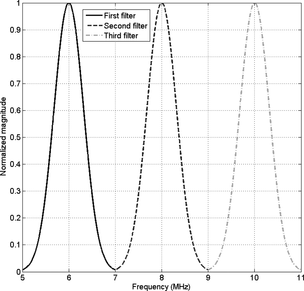
where j is the index of the Gaussian filter, i.e. j varies from 1 to K Gaussian filters. If the Gaussian filters do not overlap, the random variables a(m) and a(n), such that m ≠ n, are independent. Fig. 1 shows a plot of 3 independent Gaussian filters for a usable frequency range from 5 MHz to 11 MHz.

Fig. 1.

Plot of 3 independent Gaussian filters.

Therefore, we can find an estimate for γ = 4dΔα by performing least linear squares on Eq. (34). The expected value and the variance of the estimate γ is given by [21]:

$$\begin{array}{c}E\left[\gamma \right]=E\left[4d\mathrm{\Delta }\alpha \right]\approx \gamma =4d\mathrm{\Delta }\alpha \hfill \\ \text{var}(\gamma )\approx \frac{1}{\mathrm{\Delta }}{\displaystyle \sum _{j=1}^K}\frac{f_c{(j)}^2}{\text{var}(a(j))},\hfill \end{array}$$ (35)

where

$$\mathrm{\Delta }={\displaystyle \sum _{j=1}^K}\frac{1}{\text{var}(a(j))}{\displaystyle \sum _{j=1}^K}\frac{f_c{(j)}^2}{\text{var}(a(j))}-{\left({\displaystyle \sum _{j=1}^K}\frac{f_c(j)}{\text{var}(a(j))}\right)}^2.$$ (36)

Using Eq. (32), we can write var(γ) as

$$\text{var}(\gamma )=\frac{(N_s+N_r)}{N_s{N}_r}\frac{1}{\left\{{\displaystyle \sum _{j=1}^K}\right[{\displaystyle \sum _{i=1}^M}{(f_i-f_c(j))}^2\left]\right\}-\frac{{\left\{{\displaystyle \sum _{j=1}^K}\right[{\displaystyle \sum _{i=1}^M}{(f_i-f_c(j))}^2]f_c(j)\}}^2}{{\displaystyle \sum _{j=1}^K}\left\{\right[{\displaystyle \sum _{i=1}^M}{(f_i-f_c(j))}^2\left]f_c{(j)}^2\right\}}}$$ (37)

As in the spectral fit method, the estimate of Δα= γ/4d is unbiased. The variance in Δα is a function of the number of averaged power spectra in the sample and the reference, the size of the time gated window, the number of frequency components in the usable frequency range and the number of Gaussian filters.

IV. Validation of the statistical analysis using numerical simulations

A. Simulation Procedure

Computer simulations with a sampling frequency of 100 MHz were used to obtain two different data sets of RF backscattered signals using a Gaussian focused beam (5 cm focal length, 0.62 mm beam width, 7.5 MHz center frequency, and 50% -3dB bandwidth on transmit). These simulation parameters are chosen because they approximate the properties of a single-element focused transducer that we use for tissue characterization experiments on phantoms and ex-vivo tissue. One data set was used as a sample while the other was used as a reference. The sample and the reference had attenuation coefficients of 0.7 dB/cm-MHz and 0.5 dB-cm-MHz, respectively. The sample scatterers were identical and uniformly distributed and had a Gaussian Form Factor with a 20 µm effective radius. The reference had uniformly distributed and identical spherical shell scatterers with 10 µm radii. The spatial pulse length is 0.2 mm (0.25 µs, 1λ). Both the sample and the reference had a scatterer density of 100 mm⁻³, corresponding to approximately 10 scatterers per resolution cell, which is adequate for fully developed speckle [25]. The sample numerical data simulates scattering from homogeneous tissues where local inhomogeneities in compressibility and density result in ultrasound scattering. Similarly, the reference numerical data simulates scattering from a tissue-mimicking phantom in which glass micro-spheres scatter incoming ultrasound signals.

In the simulations, 3000 independent echo lines were generated for the sample and the reference. Each RF echo line was gated with a rectangular window centered at the focus. The power spectrum of each time gated window is approximated by taking the Fourier Transform of the RF data and squaring the magnitude of the result. In order to operate above the noise floor, the usable frequency range was selected to be the frequencies that are above the noise floor.

B. Validation of the spectral-fit statistical analysis

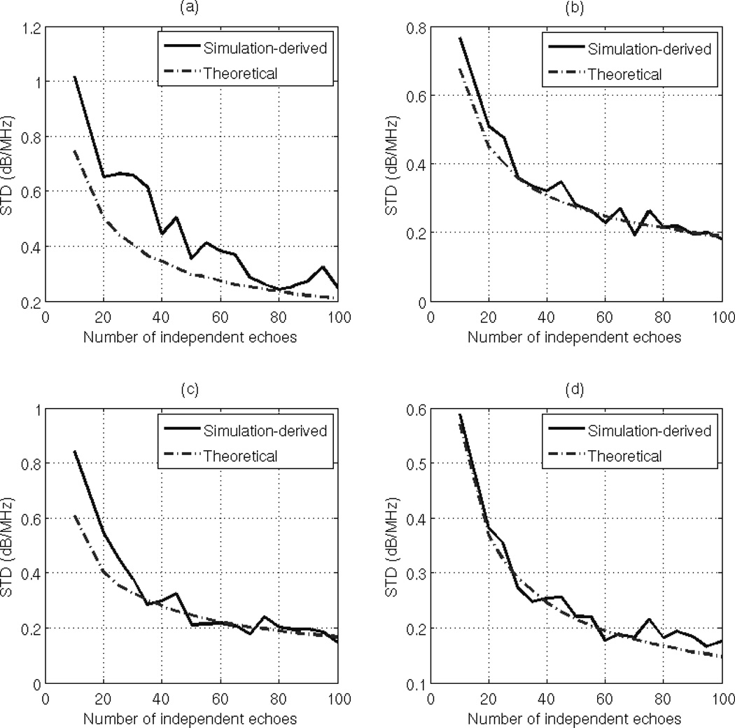
The variance in dα_s, the estimate of the attenuation coefficient in the sample multiplied by the distance from the transducer surface to the center of the ROI, is equal to the variance in dΔα which is given by (26). As discussed before, given a tissue mimicking phantom with a constant attenuation coefficient and an ultrasound system with a fixed bandwidth, the only parameter that affects the variance of the estimate dα_s is the ROI size, i.e. the number of averaged periodograms in the sample and the reference, and the size of the time gated window. To validate Eq. (26), we varied the ROI width from 10 to 100 independent echo lines in steps of 10 echo lines i.e. N_s= N_r = 10:10:100, and varied the ROI length from 1 to 20 pulse lengths in steps of 1 pulse length. We obtained 30 estimates for each combination. At each combination of ROI length and ROI width, we used the usable frequency range to calculate the theoretical variance of the estimate dα_s using Eq. (26). The theoretical standard deviation (dB/MHz) is obtained by taking the square root of the result. At each combination of ROI length and ROI width, we compared the standard deviation of the 30 estimates of dα_s to the theoretical standard deviation. Fig. 2 (a), (b), (c), and (d) shows plots of the simulation-derived and theoretical standard deviations of the estimate dα_s with respect to the number of independent echoes per ROI with an ROI length of 5, 10, 15, and 20 pulse lengths, respectively. Based on this figure, the theoretical standard deviation in the estimate dα_s is very similar to the simulation-derived standard deviation. The slight difference between the simulation-derived and the theoretical standard deviations in Fig. 2 (a) is due to the windowing effects which are more apparent at small time gated windows.

Fig. 2.

Plots of the simulation-derived and theoretical standard deviations of the estimate dα_s, which was obtained using the spectral fit method with an ROI length of (a) 5 pulse lengths (b) 10 pulse lengths (c) 15 pulse lengths (d) 20 pulse lengths, with respect to the number of independent of echoes per ROI.

C. Validation of the multiple-filter statistical analysis

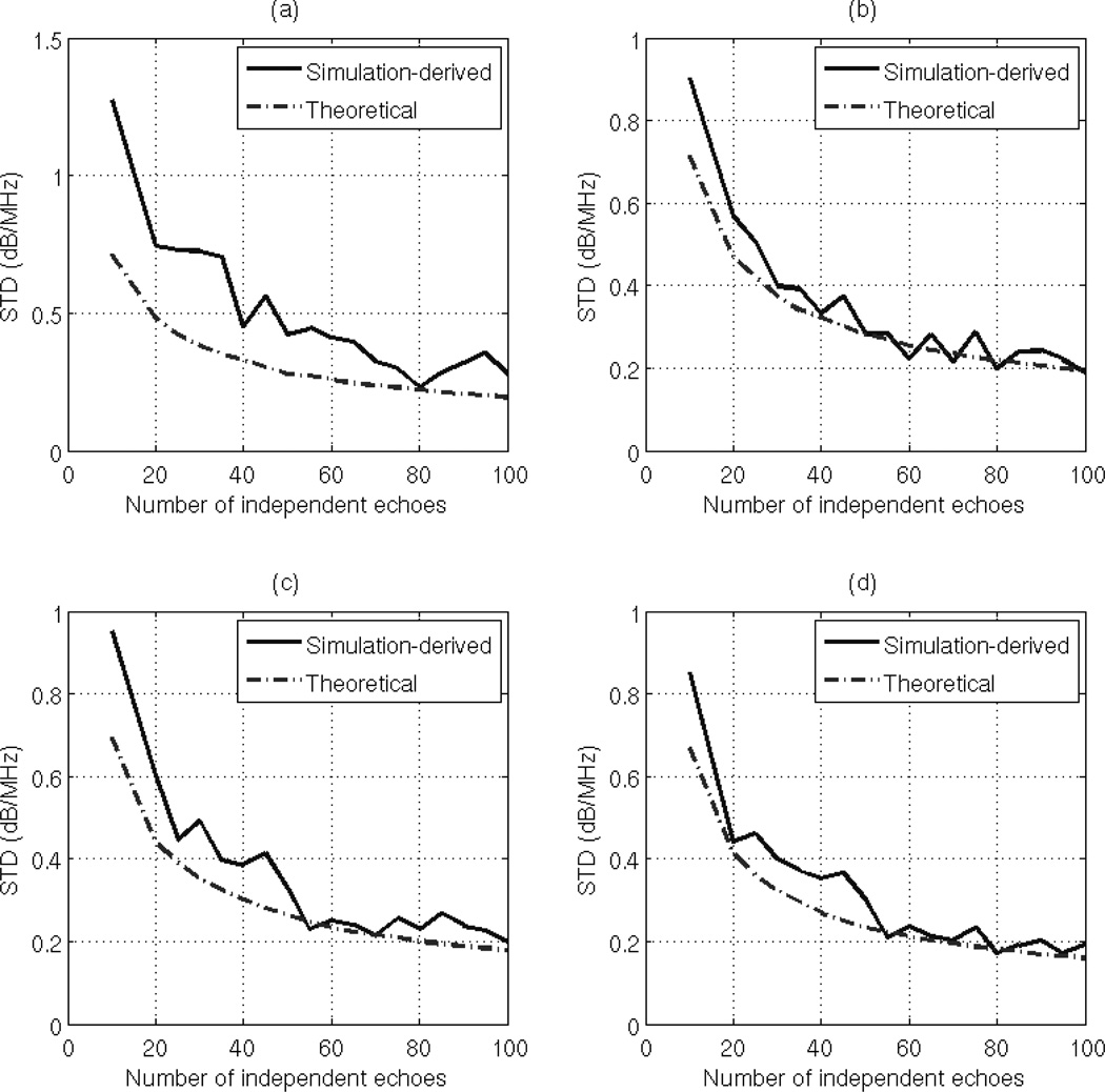
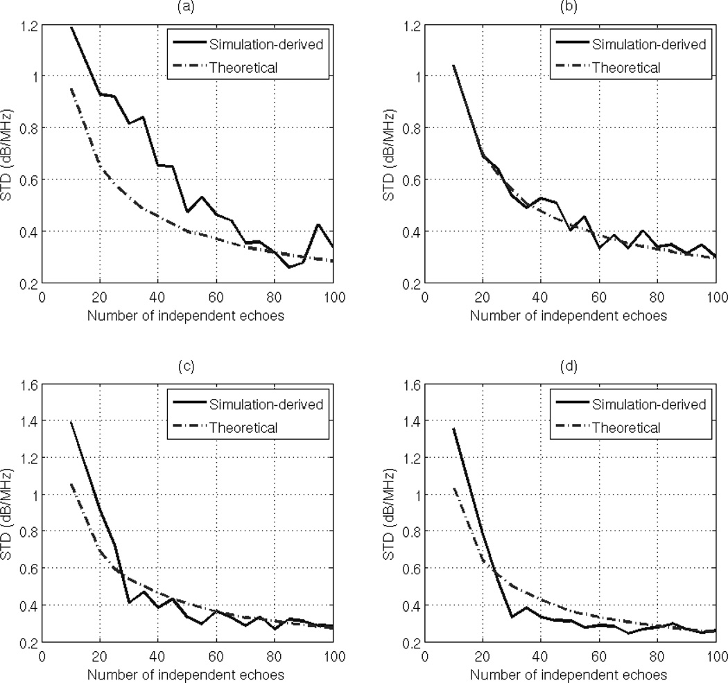
To test the validity of Eq. (37), we varied the ROI width from 10 to 100 independent echo lines i.e. N_s = N_r= 10:10:100, the ROI length from 1 to 20 pulse lengths, and the number of Gaussian filters from 2 to 10 filters, and we obtained 30 estimates of dα_s for each combination. At each combination of ROI length, ROI width, and number of Gaussian filters, we used the measured usable frequency range to calculate the theoretical variance of the estimate dα_s using Eq. (37). The theoretical standard deviation (dB/MHz) is obtained by taking the square root of the result. At each combination of ROI length and ROI width, and number of Gaussian filters, we compared the standard deviation of the 30 estimates of dα_s to the theoretical standard deviation. Fig. 3 (a), (b), (c), and (d) shows plots of the simulation-derived and theoretical standard deviation of the estimate dα_s with respect to the number of independent echoes per ROI for an ROI length of 5, 10, 15, and 20 pulse lengths, respectively and with 2 Gaussian filters. Fig. 4 (a), (b), (c), and (d) shows plots of the simulation-derived and theoretical standard deviation of the estimate dα_s with respect to the number of independent of echoes per ROI with an ROI length of 5, 10, 15, and 20 pulse lengths, respectively and with 4 Gaussian filters. Based on these figures, the theoretical standard deviation in the estimate dα_s is very similar to the simulation-derived standard deviation. As mentioned before, the slight difference between the simulation-derived and the theoretical standard deviation in plots (a) is due to the windowing effects which are more apparent at small time-gated windows.

Fig. 3.

Plots of the simulation-derived and theoretical standard deviations of the estimate dα_s, which was obtained using the multiple filter method with 2 Gaussian filters and an ROI length of (a) 5 pulse lengths (b) 10 pulse lengths (c) 15 pulse lengths (d) 20 pulse lengths, with respect to the number of independent of echoes per ROI.

Fig. 4.

Plots of the simulation-derived and theoretical standard deviation of the estimate dα_s, which was obtained using the multiple filter method with 4 Gaussian filters and an ROI length of (a) 5 pulse lengths (b) 10 pulse lengths (c) 15 pulse lengths (d) 20 pulse lengths, with respect to the number of independent of echoes per ROI.

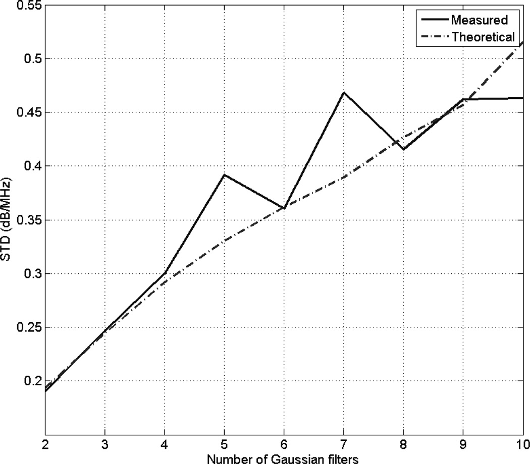
By comparing Fig. 3 and Fig. 4, we observe that for a specific ROI length and ROI width, the variance in the estimate of dα_s is smaller when the number of Gaussian filters is two compared to when the number of Gaussian filters is four. To test the dependence of the multiple filter algorithm on the number of Gaussian filters, we fixed the ROI length to 15 pulse lengths, the ROI width to 60 independent echo lines, and we plotted the simulation-derived and theoretical standard deviations of the estimate dα_s with respect to the number of Gaussian filters as shown in Fig. 5. Based on this figure, we observe that standard deviation in the estimate dα_s increases with increasing number of Gaussian filters. Therefore, the optimal number of Gaussian filters for the multiple-filter algorithm is equal to 2 when the filters are independent.

Fig. 5.

Plots of the simulation-derived and theoretical standard deviation of the estimate dα_s, which was obtained using the multiple filter method with an ROI length 10 pulse lengths and an ROI width of 60 independent echo lines, with respect to the number of Gaussian filters.

V. COMPARISON OF THE SPECTRAL FIT METHOD AND THE MULTIPLE FILTER METHOD

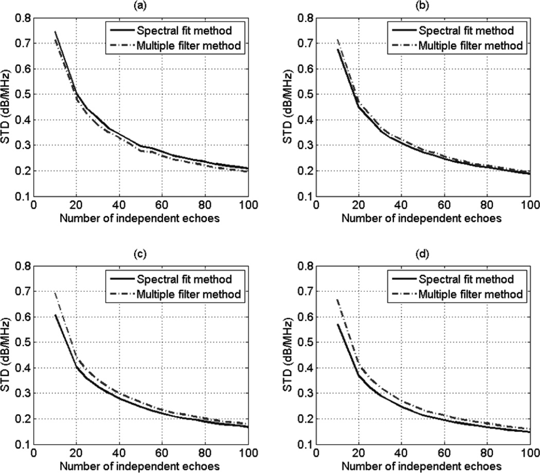
The derived expressions for the variance in the attenuation coefficient estimates (ACEs) that are obtained using the spectral fit method (see Eq. (26)) and the multiple filter method (see Eq. (37)) are not easily interpreted. Therefore, in order to compare these two equations, we used the simulation data that was described above and we varied the axial ROI size from 5 pulse lengths to 20 pulse lengths, and the lateral ROI size from 10 to 100 independent echo lines. For each ROI, the corresponding parameters (the number of averaged spectra and the number of usable frequency components) were used in (26) and (37) to obtain the theoretical variance in the ACEs. Fig. 6 shows plots of the theoretical standard deviation of the estimates dα_s versus the number of independent echoes per ROI for an axial ROI size of 5 pulse lengths, 10 pulse lengths, 15 pulse lengths, and 20 pulse lengths, respectively. Based on Fig. 6, the STDs in the ACEs that are obtained using the spectral fit method are comparable to the STDs in the ACEs that are obtained using the multiple filter method. Fig. 6 also shows that for both attenuation estimation algorithms, the variance in the ACEs has a larger dependence on the lateral ROI size than the axial ROI size. For example, if the axial ROI size is doubled there is less than a 10% decrease in the STD of the ACEs, however; if the lateral ROI size is doubled the STD in the ACEs decreases by nearly 40%.

Fig. 6.

Plots of the theoretical standard deviation of the estimate dα_s,which was obtained using spectral fit method and the multiple filter method with 2 Gaussian filters with an ROI length of (a) 5 pulse lengths (b) 10 pulse lengths (c) 15 pulse lengths (d) 20 pulse lengths, with respect to the number of independent of echoes per ROI.

VI. Discussion and Conclusion

In this paper, we performed statistical analysis on the spectral-fit method and the multiple-filter method for estimating the total attenuation along the propagation path. We found that both estimators are unbiased and that the variance in the total attenuation coefficient estimates depends on the number of frequency components in the usable frequency range (transducer bandwidth and axial ROI size), the number of independent echoes per ROI (Lateral ROI size), and the number of independent Gaussian filters in the multiple filter method. The number of frequency components in the usable frequency range is a function of the transducer bandwidth, and the size of the time gated window (ROI length in the axial direction). Note that for given ROI size and usable frequency range, both methods yield similar computation time for obtaining an estimate of the attenuation coefficient.

One important assumption in the two algorithms is that the region of interest must be homogeneous. Tissue inhomogeneities resulting from regions of mixed tissues or specular reflectors will reduce the accuracy of the algorithms. In a recent paper [26], we have shown that the error in the attenuation coefficient estimates increases with increasing variance in the scatterer number density and the scatterer size within the ROI. Currently, none of the algorithms for estimating ultrasound attenuation along the propagation path consider tissue inhomogeneities. Nevertheless, this problem is of significant importance and is the subject of an ongoing study. Another important aspect that hasn’t been addressed before is the effect of tissue motion on the accuracy of the algorithms. However, we know that tissue motion leads to a decorrelation of the ultrasound echoes resulting in an increase in the number of independent echoes per ROI. Therefore, tissue motion will likely improve the performance of the algorithms.

We have shown that for the multiple filter method, the optimal number of Gaussian filters is 2 when the filters are independent. Furthermore, the spectral fit method and the multiple filter method with 2 independent Gaussian filters yield comparable results in terms of the bias and the standard deviation of the total attenuation coefficient estimates. In the derivation of the variance in the ACEs using the multiple filter method, we assumed that the Gaussian filters are independent. However, using overlapping Gaussian filters may give better results than using only two independent Gaussian filters. Due to the correlation in the spectra that results from using overlapping Gaussian filters, it is difficult to obtain an expression for the variance in the ACEs. This variance however, can be explored using computer simulations.

In previous studies of the multiple filter method [13, 15], Bigelow used four overlapping Gaussian filters. Three of the four Gaussian filters had center frequencies that formed 4 equally spaced intervals within the usable frequency range. The fourth Gaussian filter spanned the entire usable frequency range and had a center frequency that corresponded to the middle of the usable frequency range. We used computer simulations to compare the spectral fit method, the multiple filter method with 2 independent Gaussian filters, and the multiple filter with 4 overlapping Gaussian filters which was used in Bigelow’s previous studies. Using the simulation data that was described above, we varied the lateral ROI size from 10 to 100 independent echo lines, the axial ROI size from 1 to 20 pulse lengths, and we obtained 30 estimates of dα_s using each method. At each combination of ROI length and ROI width, we compared the bias, the standard deviation, and the mean square error (MSE) in the 30 estimates of dα_s that are obtained using each method.

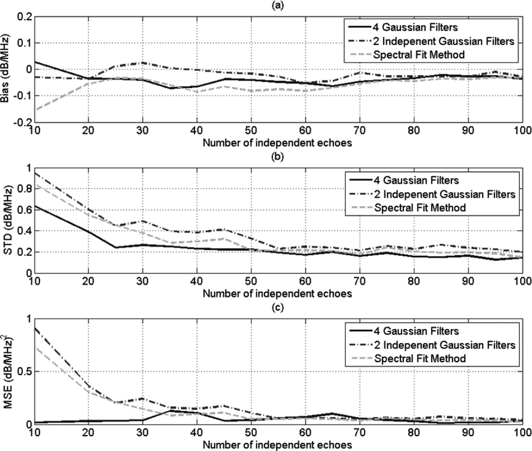
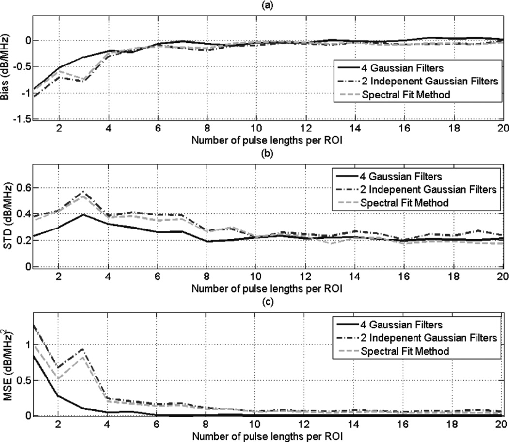
Fig. 7 (a), (b), and (c) shows plots of the bias, STD, and MSE, respectively, of the estimates dα_s versus the number of independent echoes per ROI for and ROI length of 10 pulse lengths. Similarly, Fig. 8 (a), (b), and (c) shows plots of the bias, STD, and MSE, respectively, of the estimates dα_s versus the number of pulse lengths per ROI and an ROI that contains 50 independent echo lines. Based on these 2 figures, the MSE is comparable for both the spectral fit method and the multiple filter method with 2 independent Gaussian filters, with the spectral fit method having a slightly smaller STD and a slightly larger bias compared to the 2 independent filter method. These two figures also show that in the multiple filter method, using 3 overlapping Gaussian filters and a fourth filter that spans the entire usable frequency yields a smaller variance in the attenuations estimates compared to using only 2 independent Gaussian filters. This result demonstrates that using 2 overlapping Gaussian filters and a third filter that spans the entire usable frequency range may give better results than using 3 overlapping Gaussian filters and a fourth Gaussian filter that spans the entire frequency range. A careful study must be done to find the optimal amount of overlap between the two Gaussian filters, and to find the optimal location of their center frequencies within the usable frequency range. The study could be done by modifying (35) to include the covariance between the random variables a(1) and a(2) (see (32)) which result from the first and the second Gaussian filters, respectively. The study may be complicated by the fact that the amount of overlap between the two Gaussian filters must be translated into a covariance between the random variables a(1) and a(2). However, computer simulations may be used to explore these issues.

Fig. 7.

Plots of the (a) bias (b) STD, and (c) MSE of the estimate dα_s, which was obtained using the multiple filter method with 3 independent Gaussian filters, the multiple filter method with 3 Gaussian filters, the multiple filter method with two independent filters, and the spectral fit method, with respect to the number of independent of echoes per ROI for an ROI length of 10 pulse lengths.

Fig. 8.

Plots of the (a) bias (b) STD, and (c) MSE of the estimate dα_s, which was obtained using the multiple filter method with 3 Gaussian filters, the multiple filter method with two independent filters, and the spectral fit method, with respect to the number of pulse lengths per ROI for an ROI that contains 50 independent echo lines.

Highlights.

• Ultrasound attenuation along the propagation path

• Spectral-fit algorithm

• Multiple-filter algorithm

References

- 1.Kuc R. Clinical Application of an Ultrasound Attenuation Coefficient Estimation Technique for Liver Pathology Characterization. Biomedical Engineering, IEEE Transactions on. 1980;vol. BME-27:312–319. doi: 10.1109/TBME.1980.326739. [DOI] [PubMed] [Google Scholar]
- 2.Oelze ML, et al. Differentiation and characterization of rat mammary fibroadenomas and 4T1 mouse carcinomas using quantitative ultrasound imaging. Medical Imaging, IEEE Transactions on. 2004;vol. 23:764–771. doi: 10.1109/tmi.2004.826953. [DOI] [PubMed] [Google Scholar]
- 3.Bigelow TA, et al. In vivo ultrasonic attenuation slope estimates for detecting cervical ripening in rats: Preliminary results. The Journal of the Acoustical Society of America. 2008;vol. 123:1794–1800. doi: 10.1121/1.2832317. [DOI] [PMC free article] [PubMed] [Google Scholar]
- 4.Parmar N, Kolios MC. Attenuation mapping for monitoring thermal therapy using ultrasound transmission imaging; Engineering in Medicine and Biology Society, 2004. IEMBS '04. 26th Annual International Conference of the IEEE; 2004. pp. 1329–1332. [DOI] [PubMed] [Google Scholar]
- 5.Parmar N, Kolios M. An investigation of the use of transmission ultrasound to measure acoustic attenuation changes in thermal therapy. Medical and Biological Engineering and Computing. 2006;vol. 44:583–591. doi: 10.1007/s11517-006-0067-8. [DOI] [PubMed] [Google Scholar]
- 6.Treece G, et al. Ultrasound attenuation measurement in the presence of scatterer variation for reduction of shadowing and enhancement. Ultrasonics, Ferroelectrics and Frequency Control, IEEE Transactions on. 2005;vol. 52:2346–2360. doi: 10.1109/tuffc.2005.1563279. [DOI] [PubMed] [Google Scholar]
- 7.Starritt HC, et al. Forces acting in the direction of propagation in pulsed ultrasound fields. Physics in Medicine and Biology. 1991;vol. 36:1465–1474. doi: 10.1088/0031-9155/36/11/006. [DOI] [PubMed] [Google Scholar]
- 8.Calle S, et al. Temporal analysis of tissue displacement induced by a transient ultrasound radiation force. The Journal of the Acoustical Society of America. 2005;vol. 118:2829–2840. doi: 10.1121/1.2062527. [DOI] [PubMed] [Google Scholar]
- 9.Tu H, et al. Attenuation estimations using envelope echo data: Analysis and simulations. Ultrasound in Medicine & Biology. 2006;vol. 32:377–386. doi: 10.1016/j.ultrasmedbio.2005.12.001. [DOI] [PubMed] [Google Scholar]
- 10.Greenleaf JF. Application of stochastic analysis to ultrasonic echoes: Estimation of attenuation and tissue heterogeneity from peaks of echo envelope. The Journal of the Acoustical Society of America. 1986;vol. 79:526–534. doi: 10.1121/1.393540. [DOI] [PubMed] [Google Scholar]
- 11.Lizzi FL, et al. Theoretical framework for spectrum analysis in ultrasonic tissue characterization. The Journal of the Acoustical Society of America. 1983;vol. 73:1366–1373. doi: 10.1121/1.389241. [DOI] [PubMed] [Google Scholar]
- 12.Hall TJ, et al. Ultrasonic measurement of glomerular diameters in normal adult humans. Ultrasound in Medicine & Biology. 1996;vol. 22:987–997. doi: 10.1016/s0301-5629(96)00142-1. [DOI] [PubMed] [Google Scholar]
- 13.Bigelow TA. Ultrasound attenuation estimation using backscattered echoes from multiple sources. The Journal of the Acoustical Society of America. 2008;vol. 124:1367–1373. doi: 10.1121/1.2949519. [DOI] [PMC free article] [PubMed] [Google Scholar]
- 14.Bigelow TA. Improved algorithm for estimation of attenuation along propagation path using backscattered echoes from multiple sources. Ultrasonics. 2009;vol. 50:496–501. doi: 10.1016/j.ultras.2009.10.011. [DOI] [PMC free article] [PubMed] [Google Scholar]
- 15.Bigelow T. Estimating the total ultrasound attenuation along the propagation path by applying multiple filters to backscattered echoes from a single spherically focused source. Ultrasonics, Ferroelectrics and Frequency Control, IEEE Transactions on. 2010;vol. 57:900–907. doi: 10.1109/TUFFC.2010.1494. [DOI] [PMC free article] [PubMed] [Google Scholar]
- 16.Bigelow TA, et al. Estimation of total attenuation and scatterer size from backscattered ultrasound waveforms. The Journal of the Acoustical Society of America. 2005;vol. 117:1431–1439. doi: 10.1121/1.1858192. [DOI] [PubMed] [Google Scholar]
- 17.Labyed Y, Bigelow T. Estimating ultrasound attenuation along the propagation path using a reference phantom. The Journal of the Acoustical Society of America. 2010;vol. 127:1731. doi: 10.1121/1.3483739. [DOI] [PMC free article] [PubMed] [Google Scholar]
- 18.Bigelow TA, O'Brien WD., Jr Impact of local attenuation approximations when estimating correlation length from backscattered ultrasound echoes. The Journal of the Acoustical Society of America. 2006;vol. 120:546–553. doi: 10.1121/1.2208456. [DOI] [PubMed] [Google Scholar]
- 19.Insana MF, et al. Describing small-scale structure in random media using pulse-echo ultrasound. The Journal of the Acoustical Society of America. 1990;vol. 87:179–192. doi: 10.1121/1.399283. [DOI] [PMC free article] [PubMed] [Google Scholar]
- 20.Insana MF, Hall TJ. Parametric ultrasound imaging from backscatter coefficient measurements: image formation and interpretation. Ultrason Imaging. 1990 Oct;vol. 12:245–267. doi: 10.1177/016173469001200402. [DOI] [PubMed] [Google Scholar]
- 21.Bevington PR. Data reduction and error analysis for the physical siences. 1969 [Google Scholar]
- 22.Chaturvedi P, Insana MF. Error bounds on ultrasonic scatterer size estimates. The Journal of the Acoustical Society of America. 1996;vol. 100:392–399. doi: 10.1121/1.415958. [DOI] [PubMed] [Google Scholar]
- 23.Marple SL. Digtital spectral snalysis with applications. Englewood Cliffs, NJ: 1987. [Google Scholar]
- 24.Yao LX, et al. Backscatter coefficient measurements using a reference phantom to extract depth-dependent instrumentation factors. Ultrasonic Imaging. 1990;vol. 12:58–70. doi: 10.1177/016173469001200105. [DOI] [PubMed] [Google Scholar]
- 25.Bigelow TA, O'Brien WD., Jr Scatterer size estimation in pulse-echo ultrasound using focused sources: Calibration measurements and phantom experiments. The Journal of the Acoustical Society of America. 2004;vol. 116:594–602. doi: 10.1121/1.1757453. [DOI] [PubMed] [Google Scholar]
- 26.Labyed Y, Bigelow TA. A theoretical comparison of attenuation measurement techniques from backscattered ultrasound echoes. The Journal of the Acoustical Society of America. 2011;vol. 129:2316–2324. doi: 10.1121/1.3559677. [DOI] [PMC free article] [PubMed] [Google Scholar]