Vignettes from the field of mathematical biology: the application of mathematics to biology and medicine

Abstract

The application of mathematical models in biology and medicine has a long history. From the sparse number of papers in the first half of the twentieth century with a few scientists working in the field it has become vast with thousands of active researchers. We give a brief, and far from definitive history, of how some parts of the field have developed and how the type of research has changed. We describe in more detail just two examples of specific models which are directly related to real biological problems, namely animal coat patterns and the growth and image enhancement of glioblastoma brain tumours.

1. Introduction

A few individuals in the distant past proposed mathematical models for a variety of biological and medical problems. One of the first, by Leonardo of Pisa (1202), was not very serious; it was an exercise in his arithmetic book, Liber abbaci. The problem is to start with a male and female pair of immature rabbits at the beginning of a breeding season. After one season they can reproduce and produce two pairs of immature rabbits. The parents then stop producing but after another season the immature rabbits produce two pairs each and then stop. The process continues  exactly in the same way. The question is to determine the number of pairs of rabbits at each reproductive period. The answer is 1 1 2 3 5 8 13 … : each number is the sum of the previous two. This well-known series is now known as the Fibonacci series: Leonardo of Pisa was renamed Fibonacci in the seventeenth century. This series arises in an astonishingly wide range of situations. For example, if you count the number of spirals on a pine cone, or on a sunflower head, the number will be a Fibonacci number. It, and others where the Fibonacci series is observed, is still a mystery as to why.

With the limit restriction on articles in this Theme Issue, it is possible to describe briefly only a very few of the numerous early contributions to the development of this field. Possibly the first serious examples of a mathematical model for a medical problem was by Bernoulli [1]. He suggested a model (a differential equation model) to quantify the effect of cow-pox inoculation on the spread of smallpox. This article gives some interesting data on child mortality and it is used to assess the practical advantages of a vaccination control programme. The concept of acquiring immunity by contact with a disease is much older. There is an ancient Chinese custom where children were made to inhale the powder made from the crusts of skin lesions of people recovering from smallpox. Had Bernoulli's paper been published in the first half of the twentieth century it would have been considered one of the great classics of the field on par with, for example, that of Lotka [2] and Volterra [3] on modelling a two-population predator–prey interaction, Fisher [4] on the genetics of natural selection, Kermack & McKendrick's [5] article on modelling epidemics, and Fisher [6] and Kolmogoroff et al. [7] who brought diffusion into their mathematical models of certain biological phenomena.

D'Arcy Thompson's monumental book On Growth and Form, first published in 1917 [8], is not specifically on mathematical modelling as such but mathematical concepts associated with morphological patterns played a major role. There had been considerable interest in it for a long time. The classic work of Saint-Hilaire [9] is a remarkable seminal example. Sainte-Hilaire was particularly interested in teratology and was probably the first to introduce the important concept of a developmental constraint to which we will come back in our further discussion. D'Arcy Thompson specifically commented on the absence of particular forms, which implies an awareness of developmental constraints. He emphasized the parallels between the study of form in physical systems and that of biological form, which presaged later papers in the field. Turing's [10] paper on the chemical basis of morphogenesis has only six references, one of which is to the second edition of D'Arcy Thompson's book (1942).

2. Early growth of mathematical biology

Although not specifically referred to as a separate discipline, research on the application of mathematical modelling in the biomedical sciences had been carried out by a small number of scientists. Recognition of its importance grew slowly in the 1950s with, for example, the classic Nobel Prize work on nerve conduction and excitation of Hodgkin & Huxley [11]. Turing's [10] foray into biology is primarily practical but essentially mathematical: he says nothing about real biology or morphogenesis. Importantly, however, he showed how a model system of reacting and diffusing chemicals in a bounded domain can result in steady-state spatial patterning of the chemical concentrations. We shall come back to this below when we discuss some applications of pattern formation models.

The late 1960s and to a greater extent the 1970s saw a major increase of interest in the field, including reaction–diffusion systems, primarily studied theoretically, such as the work by Prigogine & Nicolis [12], who reintroduced Turing's [10] paper, essentially ignored until then. They proposed a simpler (mathematically) model system. Another influential activator–inhibitor reaction–diffusion system was proposed by Gierer & Meinhardt [13] also based on Turing's chemical patterning concept.

Other than the above, research directly associated with the experiment was rarer. Murray [14] introduced a model for enzyme kinetics based on oxygen diffusion into pea nodules. The importance of myoglobin and haemoglobin in facilitating oxygen in a variety of physiological situations was modelled and related to the experiment by Murray [15,16] and Murray & Wyman [17]. The practical work of Winfree [18–21] on biological clocks had a major influence on the field. Among his many original results there is a practical method for resetting one's biological clock after long flights across several time zones. A brief survey of just some of the early work in this interdisciplinary field, now known as mathematical biology or theoretical biology, and lately systems biology, and its remarkable growth since the early 1970s is included in the book by Murray [22]. Research on theoretical models in ecology and epidemiology had also been growing from the 1950s: see the major review article by Levin [23,24], who specifically focuses on pattern and scale in ecology. In the mathematical modelling here, the ‘reaction’ terms model population growth and interaction or, in epidemiology, disease virulence and spread: see, for example, Grenfell et al. [25].

With the ever increasing number of people getting involved in the field the number of genuinely practical examples has grown, as has the number of essentially mathematics papers where the primary interest is in mathematics with scant connection to any real biology. By the mid-1980s it was becoming more widely recognized that any real contribution to the biological sciences from modelling must genuinely be interdisciplinary and hence related to real biology. The best research was that which proposed models for specific biological situations and with which its predictions were confirmed, or otherwise, by experiment and, importantly, help our understanding of the real biological problems. It is possible to mention only a very few of the now numerous successful interdisciplinary collaborations. There are however, many books of author-contributed chapters and of various meeting proceedings which give a good picture of how the field developed, for example those by Brenner et al. [26], Jäger & Murray [27], Levin [28], Chaplain et al. [29] and Maini & Othmer [30]. One relatively recent and important growth area is in physiology, the definitive text of which is by Keener & Sneyd [31].

3. Modelling biological pattern and form

In spite of the enormous amount of research and the exploding growth of genetics, the development of spatial pattern and form is still one of the central issues in embryology. In the past 20–30 years, it has spawned exciting, important and genuine interdisciplinary research between theoreticians and experimentalists, the common aim of which is the elucidation of the underlying mechanisms involved in embryology and medicine; most of these mechanisms are essentially still unknown.

By way of illustration, we shall describe some specific biological problems and their modelling. We shall point out some of the limitations of Turing-type reaction–diffusion mechanisms which necessitated a new, and more experimentally verifiable, approach to biological pattern formation, known as the mechanical theory of biological pattern formation proposed by Oster et al. [32], Murray et al. [33] and Murray & Oster [34]. A large body of research has been developed on tumour growth, such as brain tumours (see [36] for a survey): it is now being used medically to quantify the efficacy of individual patient treatment scenarios prior to their use.

The first genuine experimentally based reaction–diffusion system which produced steady-state chemical spatial patterns in line with Turing's predictions was developed by Thomas [37]. Interestingly, when you take all of these model systems and look at the parameter ranges which can generate spatial patterns [38], by far the largest ranges are those of the practical system proposed by Thomas [37]. There are numerous review articles and books—for example, Murray's Mathematical Biology [35,36,39]—which describe, among many other topics, Turing's theory of morphogenesis and its influence on modelling biological pattern and form in detail and, more specifically, Turing's theory in a review article [40]. Maini [41], in his review, specifically addresses pattern and form.

Since the late 1990s there has been an ever increasing number of truly interdisciplinary studies which cover a remarkably wide spectrum of topics such as wound healing and cancer to mention just two (see [35,36] for a survey). Much of this involves modelling the phenomena across many different scales. One example is the seminal work of Gatenby et al. [42]. The suggestion here was that tumour cells create an environment which allows certain mutations to be selected and hence the evolution of mutant cell populations to occur within the body; this is called somatic evolution. The authors analysed somatic evolution in this context and showed a number of evolutionary pathways in ductal carcinoma in situ. Colleagues suggested that different mutant clones would emerge in a well-defined temporal sequence, while the mathematical simulations showed that this was highly unlikely. The simulations predicted that hypoxia (lack of oxygen) should promote emergence of varying sized nodules of a mutant clone of a certain type surrounded by other cell types, and that over time these nodules would grow and merge. This stimulated their colleagues to carry out experiments which confirmed this prediction. Another study highlights cellular adaptions of cancer cells in colorectal cancer [43].

The basic concept, which Turing demonstrated mathematically, was that if you have two chemicals, in later studies (such as [13]) referred to as an activator and an inhibitor, which react together and at the same time diffuse, crucially at different rates with the inhibitor having the larger diffusion coefficient, it is possible for such a coupled system of reaction–diffusion equations to produce steady-state spatial patterns in chemical concentrations of the reactants. In the early to mid-1970s Turing's paper was rediscovered by more theoreticians with an increasing number of publications starting to appear. Closely related, but not specifically to Turing's work, is the seminal experimental work on the importance of chemical gradients in embryonic development by Wolpert [44], who introduced the concept of ‘positional information’, where cells in a chemical gradient react to a chemical concentration with which they are associated. His work initiated a huge amount of experimental and theoretical work, often controversial, that is still going on. For a review of his work and his views on development, see Wolpert's [45] book on the principles of development.

To get an intuitive idea of how the reaction–diffusion patterning works, consider the following, albeit unrealistic, scenario of a field of dry grass in which there is a large number of grasshoppers which can generate a lot of moisture by sweating if they get warm. Now suppose the grass is set alight at several random points and a flame front starts to propagate from each. We can think of the grasshopper as an inhibitor and the fire as an activator. If there were no moisture to quench the flames the fires would simply spread over the whole field, which would result in a uniform charred area. Suppose, however, that when the grasshoppers get warm enough they can generate enough moisture to dampen the grass so that when the flames reach such pre-moistened areas the grass will not burn. The scenario for a heterogeneous spatial pattern of charred and uncharred grass patches is then the following. The fires start to spread; these represent one of the ‘reactants’, the activator, with a fire ‘diffusion’ coefficient, which quantifies how fast the fire spreads. When the grasshoppers, the inhibitor ‘reactant’, ahead of the flame fronts feel it coming they move quickly ahead of it; that is, they have a ‘diffusion’ coefficient which is much larger than that of the fire fronts. The grasshoppers then sweat profusely and generate enough moisture to prevent the fires spreading into the moistened area. By this way, the charred areas are restricted to finite domains which depend on the ‘diffusion’ coefficients of the reactants—fire and grasshoppers—and the various ‘reaction’ parameters. If the grasshoppers and flame fronts ‘diffused’ at the same speed, no such spatial pattern could evolve.

4. How the leopard gets its spots

Murray [46] studied how animal coat patterns were formed and used the practical Thomas [37] reaction–diffusion mechanism to study them. Murray showed that a single pre-patterning mechanism was capable of generating the geometry of mammalian coat patterns, from the mouse to the badger to the giraffe to the elephant and almost everything in between, with the end pattern governed simply by the size and shape of the embryo at the time the pattern formation process was initiated. In solving the reaction–diffusion system the domain size and shape is crucial. For a given mechanism if you try and simulate solutions in a very small domain with zero flux boundary conditions it is not possible to obtain steady-state spatial patterns. A minimum size is needed to drive any sustainable spatial pattern. If, for example, it is a long thin domain, you can only generate stripes. You can think about it intuitively. Consider a long thin tank into which you throw a stone at one end: the only waves which persist are one dimensional along the tank. If the tank is both long and wide, a pond for example, and the surface is disturbed, it is possible to have more complex two-dimensional surface wave patterns.

In the calculations, a set of reaction and diffusion parameters were chosen for the Thomas [37] system which could produce a diffusion-driven instability and keep them fixed for all the calculations. Only the scale and geometry of the domain were varied. In the figures below, the resulting pat­terns are coloured dark and light in re­gions where the concentration of one of the morphogens is greater than or less than the concentration in the ho­mogeneous steady state. Even with such limitations on the parameters, the wealth of possible patterns is remarkable. For a given domain size and geometry each set of initial conditions gave a similar but, crucially, unique pattern.

Suppose the surface, which corresponds to the reaction–diffusion domain, is a rectangle. As mentioned, if the surface is very small, it cannot have any spatial pattern: a minimum size is therefore needed to exhibit spatial heterogeneity. As the size of the rectan­gle is increased, a series of increasing­ly complex spatial patterns emerge.

The concept behind the model is that the simulated spatial patterned solutions of a reaction–diffusion mechanism reflect the final morphogen melanin landscape observed on animal coats [36,39,46–48]. With this scenario the cells react to a given level in morphogen concentration, thus producing melanin (or rather becoming melanocytes—cells which produce melanin). In figures 1a and 2a, the black regions represent high levels of melanin concentration. It should be emphasized that this model is a hypothetical one which has not been verified experimentally but rather circumstantially. The main purpose is to show how scale and shape play major roles in animal coat patterns as they must in other developmental processes. Such an approach has also been used in lepidopteran wing patterns [39,47,49]. Importantly, the latter work presents experimental confirmation of their theoretical predictions.

Figure 1.

(a) Examples of a developmental constraint. Spotted animals can have striped tails but not the other way round. From left to right: the drawings are typical of the tail of the leopard, the cheetah and the genet together with the solutions from a reaction–diffusion system which can generate steady-state spatial patterns. The geometry and scale when the pattern mechanism is activated play crucial roles in the resulting coat patterns. Dark regions represent areas of high morphogen concentration. (Tail art work reproduced with permission of Patricia Wynne.) (b) A cheetah (Acinonyx jubatus) in the Serengeti: an example of the developmental constraint described in (a). (Photograph courtesy of Professor Andrew Dobson.)

Figure 2.

(a) These show the result of numerical simulations of the reaction–diffusion model proposed for the generation of coat markings on animals; it is the same mechanism used in figure 1. The model parameters were also the same; only the scale parameter was varied. The domain sizes have been reduced to fit in a single figure but in the simulations there was a scale difference of 1000 between the smallest and the largest figure. (b) An example of the first bifurcation: Valais blackneck goat. (Photograph courtesy of B. S. Thurner Hof, Wikimedia Commons.)

An example of how the geometry constrains the possible pattern modes is when the domain is so narrow that only simple, essentially one-dimensional, modes can exist. Two-dimensional patterns require the do­main to have enough breadth as well as length. Consider a tapering cylinder. If the radius at one end is large enough, two-dimensional patterns can exist on the surface. So, such a tapering cylinder can exhibit a gradation from a two-di­mensional pattern to simple stripes as in figure 1a.

The solutions of the reaction–diffusion system in domains shown in figure 1 were first computed. These domains all taper as shown. This shows that the conical domain mandates that it is not possible to have a tail with spots at its tip and stripes at its base, but only the converse: figure 1 shows some examples of specific animal tails. This is a genuine example of a developmental constraint. Cheetahs are prime examples of this, as well as other spotted animals. Geoffrey's cat (Leopardus geoffroyi), named after Geoffroy Saint-Hilaire who travelled extensively in the south and east of South America, the habitat of this animal, is a less well-known example of a spotted cat on which both the tail and the legs exhibit the developmental constraint. If the threshold level of morphogen is slightly different then a qualitatively similar pattern will develop. In this way quite different, but globally similar, patterns can be formed and could be the explanation for the different types of patterns on different species of the same animal genre, such as the giraffe.

The interpretation of figure 2 is that if the animal skin size is too small when the patterning mechanism is activated, as in the mouse, or too large, as in the hippopotamus and elephant, then no clear pattern will be observed and these animals are essentially uniform in colour. In between there is a progressively more complex pattern as the size increases: the first two bifurcations are illustrated in figure 2 with the larger animals still showing coat pattern but looking progressively uniform in colour as shown in figure 2a.

Note the patterning where the rear leg joins the body in figure 3b. This is typical of the model simulations [36,39,48]. Since the final pattern is dependent on when in development the patterning mechanism is activated and on the random initial conditions every animal's coat pattern is unique. The wider and fewer stripes on the zebra Equus burchelli is a result of a different timing for pattern initiation as discussed in detail by Murray [36,39]. Although rare, aberrations, such as striped black sheep, black zebras with white stripes and so on, occur [36]: these are probably the result of a genetic mutation. The possible survival of these two specific zebra species is quite different and is discussed in detail in an interesting article by Rubenstein [50].

Figure 3.

Photographs of animals which exhibit subsequent bifurcating patterns: (a) belted Galloway cows. (Photograph courtesy of Allan Wright.) (b) Typical scapular striping on a Grévy zebra (Equus grevyi). (Photograph courtesy of Professor Daniel Rubinstein.)

There have been numerous developments and an increased understanding of how coat patterns on animals, fish and butterflies, for example, are formed with the addition and combination of other pattern-forming mechanisms, such as chemotaxis whereby there is a movement of cells upward in the chemical gradients. There are numerous review articles and books. For example, Baker et al. [51] discuss somite formation, Painter et al. [52] consider fish stripe formation through chemotaxis, Camazine et al. [53], Maini [41,54], Suzuki et al. [55] and Kondo et al. [56] discuss evolving fish patterns and other patterned species.

In an interesting paper, Allen et al. [57] point out that an understanding of the diversity of animal coat patterns requires an understanding of both the mechanisms which create them and their adaptive value. Among other things they discuss the advantages of specific patterns in different environments. They use a reaction–diffusion model but their conclusions are general and do not rely on specific reaction–diffusion models. They convincingly show how different markings relate to specific natural environments for the specific fields.

5. Glioblastoma brain tumours—enhancing imaging and highlighting problems of current treatment

A practical application of mathematical modelling that is proving to be of significant medical use is in the growth and control of glioblastomas, the most aggressive brain tumours, which are always fatal, irrespective of any of the current treatments. Tracqui et al. [58] and Cruywagen et al. [59] were the first to propose a basic model, the analyses of which have proved medically illuminating. Woodward et al. [60] showed the behaviour of surgically treated high-grade gliomas to a degree of accuracy which had not been possible in vivo with statistically significant probability even with groups of more than 50 real patients [61]. Burgess et al. [62] developed the three-dimensional model which is the basis for subsequent three-dimensional models currently used. This paper reconfirmed the limitations of existing imaging techniques, the limitations of which still exist. Burgess et al. [62] were also the first to demonstrate that cancer cell diffusion, mainly ignored up to that time, is a major component of glioma growth. They showed that only those tumours with a low diffusion rate could benefit from wide surgical resection, although eventually there will always be multi-focal recurrence as was made clear in their study.

The practical basic mathematical model (a full review is given by Murray [36]) encompasses the two key elements in the growth of tumours, namely the invasive diffusive properties of the cancer cells and their growth rate. Qualitatively, the model is stated as

5.1

the mathematical form of which is

5.2

where c (x, t) is the glioma cell density, measured in cells mm⁻³, at position, x, in the brain at time, t, measured in months, D(x) is the cell diffusion (invasion), measured in mm² per month, which quantifies the invasiveness of the cancer cells at position x in the brain and ρ is the net proliferation rate (per month) of the cancer cells which gives the cell turnover time as log 2/ρ (months).

Using the model, two individual patient brain scans allow the key model parameters, namely the diffusion, D, and the cell growth, ρ, to be calculated [63,64]. With these parameter values we can predict the growth of such brain tumours and importantly estimate key aspects of the tumour's growth and response of individual patients to different treatment protocols prior to their use. Figure 4 is a computed solution of equation (5.2) in an anatomically correct brain: it shows the detectable tumour at death and the spread of the tumour cells beyond what can be detected by the most accurate current computed tomography (CT) or magnetic resonance imaging (MRI) techniques. Simulations of the model thus greatly enhance current imaging techniques to whatever level of cancer cell density is required. The model analysis shows how fast the tumour grows and, importantly, where in the brain [64,65].

Figure 4.

Computed solutions of equation (5.2) in a three-dimensional anatomically accurate brain. These show the horizontal section of the virtual human brain through the site of the original tumour (`plus’ in (a), `asterisk’ in (b)). The left image in each is the tumour at diagnosis while the right image is the same tumour at the time of death. The thick black contour defines the edge of the tumour that can be detected by enhanced CT. The blue contours outside this black line represent lines of constant cancer cell densities peripheral to the imaging limits. (a) Tumour in grey matter: the time from diagnosis to death is approximately 8 months. (b) Tumour in white matter: the time from diagnosis to death is approximately 5 months. (Figures adapted from [64].)

When a glioma is detected it has been growing for many months. From the scans of the anatomically correct patient brain the volume of an equivalent sphere of radius r is calculated. For a large time, t, the solution of (5.2) gives (see [35,36]) the approximate radius of detectable tumour and the velocity of growth, v, as approximately

5.3

That is, the equivalent radial growth is linear in time, a finding confirmed by Mandonnet et al. [66].

If we consider that detection is when the equivalent spherical tumour volume is typically of radius 15 mm and that death occurs when the radius is 30 mm [64,65] the approximate survival time from detection, in the absence of any treatments, is given, from (5.3), by

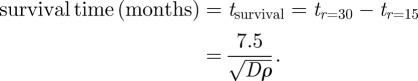5.4

Typical growth rates vary quite widely, approximately from 1 to 5/month and diffusion rates from 1 to 8 mm²/month.

Survival time, however, depends on where the tumour is mainly situated. If it is primarily in the grey area of the thalamus, for example, the diffusion is smaller and so the survival time is longer, as is clear from the expression (5.4).

Mathematical analysis of the model equation shows that the approximate equivalent diameter of the tumour and the steepness of the cancer cell density at its approximate edge, which determines the area of surgical removal (resection), are given by

5.5

The smaller the diffusion coefficient the steeper the edge of the tumour and the smaller the thickness, which implies that more of tumour can be removed surgically. Surgery, never successful, can be directly incorporated into the model (5.2), as was originally done by Woodward et al. [60]. By the same token, radiation can also be included and more precise radiation is also possible. Both of these result in a longer life expectancy than for larger diffusion coefficients since it takes longer for recurrence to occur from the remaining cancer cells outside the resection volume. The analysis of this basic model provides genuine medical information that enhances the efficacy of current therapies and, crucially, that enables them to be quantified for individual patients prior to their use (e.g. [65]). Among other things, figure 4 also clearly shows why regrowth of the tumour is inevitably multifocal after surgery.

6. Concluding discussion

This has been a very short and personal choice from the vast literature associated with the application of mathematical models in the biomedical sciences. In the 1980s with most of the research conclusions being speculative there was a decrease in the new applications of reaction–diffusion models since demonstrating the existence of specific morphogens was proving elusive. This resulted in the new mechano-chemical theory of biological pattern and form, mentioned above, which was based on experimental data on real cells and the forces they could exert in the generation of pattern and form. From the mid-1990s on the practical use of reaction–diffusion models has again increased as has research and developments of the Oster–Murray mechano-chemical theory of pattern formation as more experimental data and confirmation of modelling predictions have been found.

These mechano-chemical models assume that cells move in response to external physical and chemical guidance cues and form spatial patterns: see Murray [36,39] for a full discussion. Oster and Murray's mechano-chemical approach directly brought forces and known measurable properties of biological tissue into the morphogenetic pattern-formation process. The mechanisms start with known experimental facts about embryonic cells and tissue involved in development. They were used to construct model mechanisms which reflect these physical facts. Basically, they took the view that mechanical morphogenetic movements themselves create the pattern and form. The models quantify the coordinated movement and patterning of populations of cells. The models are based on the experimental observations that early embryonic dermal cells are capable of independent movement and have the ability to generate traction forces through long finger-like protrusions called filopodia. These can attach to adhesive sites on the tissue's extracellular matrix (ECM) and thus pull themselves along; at the same time they deform the ECM. This cell traction is resisted by the viscoelasticity of the ECM. The orchestration of the various physical effects can generate spatial aggregation patterns in cell number density and the models show how the parameters affect the size and shape of the patterns and when they can form. Here, pattern formation and morphogenesis occur simultaneously as a single process. Work on these models has resulted in understanding and suggesting numerous examples of developmental constraints and morphogenetic rules, which have been confirmed by the experiment and have suggested new avenues of research: see, for example, Alberch [67,68], Alberch & Gale [69] and Shubin & Alberch [70].

Despite the major developments in the past 20 years, although we now know a lot more about pattern development, most mechanisms are still not fully understood. We do not know, for example, the complete mechanisms of how cartilage patterns in developing limbs are formed, or the specialized structures in the skin such as feathers, scales, glands and hairs, or the myriad of widely observed patterns. Many of the rich spectrum of spatial patterns observed in development evolve from a homogeneous mass of cells which are orchestrated by genes which initiate and control the pattern-formation mechanisms: genes themselves are not involved in the actual physical process of pattern generation. The basic philosophy behind practical modelling in biology is to try to incorporate the physico-chemical events, which from observation and experiment appear to be going on during development, within a model mechanistic framework which can then be studied mathematically and, importantly, the results related back to the biology. These morphogenetic models provide the embryologist with possible scenarios as to how, and when, the pattern is laid down, how elements in the embryo might be created and what constraints on possible patterns are imposed by different models. Many of the references in this article have greatly increased our biological understanding.

Both the mechano-chemical models and reaction–diffusion models have been fruitfully applied to a vast range of biological problems in morphogenesis and elsewhere, including feather primordia arrangement, wound healing, wound scarring, cartilage formation, shell and mollusc patterns and many others. It is almost certain that both mechanisms are involved in development and although they are in a sense competing theories we do not think of them as such but rather mechanisms which complement each other. Perhaps the most fundamental difference between the theories is that the elements involved directly in the mechanical theory are all real biological quantities, namely cells, tissue and the forces generated by the cells. All quantities involved are measurable. In the end, however, the key aspect of these mechanisms is their ability to predict the subsequent form and pattern, which can be verified experimentally.

The final arbiter of a model's correctness and usefulness is not in what biological patterns it generates (although a first necessary condition for any such model is that it must be able to produce biologically observed patterns), but in how consistent it appears in the light of subsequent experiments and observations.

The explosion in biochemical techniques over the last several decades has led to a still larger increase in our biological knowledge, but has partially eclipsed the study of the intermediate mechanisms which translate gene influence into chemicals, into gradients, and into pattern and form. As a result, there is much still to be done in this area, both experimentally and theoretically.

As seen in many of the papers referred to here, models and their biological predictions encouragingly have been a major stimulant for guiding critical experiments which have resulted in significant discoveries. This, of course, should be the aim of any mathematical biology modelling, namely to stimulate in any way whatsoever any endeavour which results in furthering our understanding of biology.

We have clearly only scratched the surface of a huge, important and ever expanding interdisciplinary world. Biology, in its broadest sense, is clearly the science of the foreseeable future. What is clear is that the application of mathematical modelling in the biological, medical, ecological and psychological sciences is going to play an increasingly important role in future major discoveries and control strategies. There is an ever increasing number of areas where theoretical modelling is important such as social behaviour, conservation in animals when their environment is changed through human land use, climate change and so on. In the case of zebras, for example, Rubenstein [50] shows, by unravelling how species adapt to specific environmental changes, such as land use, why the Grévy zebra (Equus grevyi: see figure 3b) is nearing extinction while another (Equus burchelli) has adapted its behaviour to survive. Behavioural ecology is another important expanding area of research. How insect swarms, bird flocks, schools of fish, animals and so on reach community decisions is another exciting, relatively new, fast growing area: see, for example, Simpson et al. [71], Buhl et al. [72] and Nabet et al. [73].

Mathematical biology now has active researchers, numbering in the thousands, in practically all of the biomedical sciences. Mathematical modelling in the social sciences is another growth area of the future. One example of their involvement is the theoretical model developed for a major study on marital interaction and divorce prediction. The basic model and its practical application is based on a model first proposed by Cook et al. [74], developed and used in a major study of 700 newly married couples: see Gottman et al. [75,76] and the book by Murray [35] for a short survey. The prediction of the future of marital stability proved surprisingly accurate, with an accuracy of 94 per cent. Its use in marital therapy is proving highly successful.

Another positive development, although still very much in its infancy and not generally accepted, is the realization that in medical training, medical trials and so on there is often a singular lack of true scientific process: the current (2011) controversy over the use of prostate specific antigen (PSA) tests and prostate cancer is just one example. A major anomaly of PSA tests has been explained by Swanson et al. [77].

A crucially important aspect of all this kind of mathematical or theoretical biological research is its genuine interdisciplinary content. There is no way mathematical modelling could solve major biological problems on its own. On the other hand it is highly unlikely that even a reasonably complete understanding could come solely from experiment.

References

- 1.Bernoulli D. 1760. Essai d'une nouvelle analyse de la mortalité causée par la petite vérole, et des avantages de l'inoculation pour la prévenir. Histoire de l'Acad. Roy. Sci. (Paris) avec Mém. des Math. et Phys. and Mém. 1–45 [Google Scholar]
- 2.Lotka A. J. 1925. Elements of physical biology. Baltimore, MD: Williams and Wilkins [Google Scholar]
- 3.Volterra V. 1926. Variazionie fluttuazioni del numero d'individui in specie animali conviventi. [Translation by R. N. Chapman. In: Animal ecology, pp. 409–448. McGraw Hill, New York, 1931], Mem. Acad. Lincei. 2, 31–113 [Google Scholar]
- 4.Fisher R. A. 1930. The genetical theory of natural selection. (Reprinted 1958) New York, NY: Dover [Google Scholar]
- 5.Kermack W. O., McKendrick A. G. 1932. Contributions to the mathematical theory of epidemics. Proc. R. Soc. Lond. A 138, 55–83 [Google Scholar]
- 6.Fisher R. A. 1937. The wave of advance of advantageous genes. Ann. Eugenics 7, 353–369 [Google Scholar]
- 7.Kolmogoroff A., Petrovsky I., Piscounoff N. 1937. Étude de l’équation de la diffusion avec croissance de la quantité de matière et son application à un problème biologique. Moscow University, Bull. Math. 1, 1–25 [Google Scholar]
- 8.D'Arcy Thompson W. 1917. On growth and form. Cambridge, UK: Cambridge University Press [Google Scholar]
- 9.Saint-Hilaire G. 1836. Traité de Tératologie, vols 1–3 Paris, France: Baillière [Google Scholar]
- 10.Turing A. M. 1952. The chemical basis of morphogenesis. Phil. Trans. R. Soc. Lond. B 237, 37–72 10.1098/rstb.1952.0012 (doi:10.1098/rstb.1952.0012) [DOI] [Google Scholar]
- 11.Hodgkin A. L., Huxley A. F. 1952. A quantitative description of membrane current and its application to conduction and excitation in nerve. J. Physiol. (Lond.) 117, 500–544 [DOI] [PMC free article] [PubMed] [Google Scholar]
- 12.Prigogine I., Nicolis G. 1967. On symmetry breaking instabilities in dissipative systems. J. Chem. Phys. 46, 3542–3551 [Google Scholar]
- 13.Gierer A., Meinhardt H. 1972. A theory of biological pattern formation. Kybernetik 12, 30–39 10.1007/BF00289234 (doi:10.1007/BF00289234) [DOI] [PubMed] [Google Scholar]
- 14.Murray J. D. 1968. A simple method for obtaining approximate solutions for a class of diffusion-kinetic enzyme problems. I. General class and illustrative examples. Math. Biosci. 2, 379–411 10.1016/0025-5564(68)90025-4 (doi:10.1016/0025-5564(68)90025-4) [DOI] [Google Scholar]
- 15.Murray J. D. 1971. On the molecular mechanism of facilitated oxygen diffusion by haemoglobin and myoglobin. Proc. R. Soc. Lond. B 178, 95–110 10.1098/rspb.1971.0054 (doi:10.1098/rspb.1971.0054) [DOI] [PubMed] [Google Scholar]
- 16.Murray J. D. 1974. On the role of myoglobin in muscle respiration. J. Theor. Biol 47, 115–126 10.1016/0022-5193(74)90102-7 (doi:10.1016/0022-5193(74)90102-7) [DOI] [PubMed] [Google Scholar]
- 17.Murray J. D., Wyman J. 1971. Facilitated diffusion: the case of carbon monoxide. J. Biol. Chem. 246, 5903–5906 [PubMed] [Google Scholar]
- 18.Winfree A. T. 1970. An integrated view of the resetting of a circadian clock. J. Theor. Biol. 28, 327–374 10.1016/0022-5193(70)90075-5 (doi:10.1016/0022-5193(70)90075-5) [DOI] [PubMed] [Google Scholar]
- 19.Winfree A. T. 1975. Resetting biological clocks. Phys. Today 28, 34–39 10.1063/1.3068875 (doi:10.1063/1.3068875) [DOI] [Google Scholar]
- 20.Winfree A. T. 1987. The timing of biological clocks. New York, NY: Scientific American Books [Google Scholar]
- 21.Winfree A. T. 2000. The geometry of biological time, 2nd edn. Berlin, Germany: Springer [Google Scholar]
- 22.Murray J. D. 1977. Nonlinear differential equation models in biology. Oxford, UK: Clarendon Press [Google Scholar]
- 23.Levin S. A. 1992. The problem of pattern and scale in ecology. Ecology 73, 1943–1967 10.2307/1941447 (doi:10.2307/1941447) [DOI] [Google Scholar]
- 24.Levin S. A. (ed.) 1994. Frontiers in mathematical biology. Berlin, Germany: Springer [Google Scholar]
- 25.Grenfell B. T., Pybus O. G., Gog J. R., Wood J. L. N., Daly J. M., Mumford J. A., Holmes E. C. 2004. Unifying the epidemiological and evolutionary dynamics of pathogens. Science 303, 327–332 10.1126/science.1090727 (doi:10.1126/science.1090727) [DOI] [PubMed] [Google Scholar]
- 26.Brenner S., Murray J. D., Wolpert L. (eds) 1981. Theories of biological pattern formation. London, UK: Royal Society [Google Scholar]
- 27.Jäger W., Murray J. D. (eds) 1984. Modelling of patterns in space and time. In Proc. Workshop on Modelling of Patterns in Space and Time, Heidelberg, Germany, 4–8 July 1983. Lecture Notes in Biomathematics, vol. 55. Berlin, Germany: Springer-Verlag. [Google Scholar]
- 28.Levin S. A. 1994. Frontiers in ecosystem science. In Frontiers in mathematical biology (ed. Levin S. A.), pp. 381–389. Lecture Notes in Biomathematics, vol. 100. Berlin, Germany: Springer-Verlag. [Google Scholar]
- 29.Chaplain M. A. J., Singh G. D., Maclachlan J. C. 1999. On growth and form spatio-temporal pattern formation in biology. New York, NY: Wiley [Google Scholar]
- 30.Maini P. K., Othmer H. G. (eds) 2001. Mathematical models for biological pattern formation mathematics and its applications. IMA, vol. 121. New York, NY: Springer [Google Scholar]
- 31.Keener J., Sneyd J. 2008. Mathematical physiology, 2nd edn. Berlin, Germany: Springer [Google Scholar]
- 32.Oster G. F., Murray J. D., Harris A. K. 1983. Mechanical aspects of mesenchymal morphogenesis. J. Embryol. Exp. Morph. 78, 83–125 [PubMed] [Google Scholar]
- 33.Murray J. D., Oster G. F., Harris A. K. 1983. A mechanical model for mesenchymal morphogenesis. J. Math. Biol. 17, 125–129 [DOI] [PubMed] [Google Scholar]
- 34.Murray J. D., Oster G. F. 1984. Generation of biological pattern and form. IMA J. Math. Appl. Med. Biol. 1, 51–75 10.1093/imammb/1.1.51 (doi:10.1093/imammb/1.1.51) [DOI] [PubMed] [Google Scholar]
- 35.Murray J. D. 2002. Mathematical biology. I. An introduction, 3rd edn. New York, NY: Springer [Google Scholar]
- 36.Murray J. D. 2003. Mathematical biology. II. Spatial models and biomedical applications, 3rd edn. New York, NY: Springer. [Google Scholar]
- 37.Thomas D. 1975. Artificial enzyme membranes, transport, memory, and oscillatory phenomena. In Analysis and control of immobilized enzyme systems (eds Thomas D., Kernevez J.-P.), pp. 115–150 Berlin, Germany: Springer [Google Scholar]
- 38.Murray J. D. 1982. Parameter space for Turing instability in reaction-diffusion mechanisms: a comparison of models. J. Theor. Biol. 98, 143–163 10.1016/0022-5193(82)90063-7 (doi:10.1016/0022-5193(82)90063-7) [DOI] [PubMed] [Google Scholar]
- 39.Murray J. D. 1989. Mathematical biology. Heidelberg, Germany: Springer [Google Scholar]
- 40.Murray J. D. 1990. Turing's theory of morphogenesis—its influence on modelling biological pattern and form. Bull. Math. Biol. 52, 119–152 10.1016/S0092-8240(05)80007-2 (doi:10.1016/S0092-8240(05)80007-2) [DOI] [Google Scholar]
- 41.Maini P. K. 2004. Using mathematical models to help understand biological pattern formation. C. R. Biol. 327, 225–234 10.1016/j.crvi.2003.05.006 (doi:10.1016/j.crvi.2003.05.006) [DOI] [PubMed] [Google Scholar]
- 42.Gatenby R. A., Smallbone K., Maini P. K., Rose F., Averill J., Nagle R. B., Worrall L., Gillies R. J. 2007. Cellular adaptations to hypoxia and acidosis during somatic evolution of breast cancer. Br. J. Cancer 97, 646–653 10.1038/sj.bjc.6603922 (doi:10.1038/sj.bjc.6603922) [DOI] [PMC free article] [PubMed] [Google Scholar]
- 43.Johnston M. D., Edwards C. M., Bodmer W. F., Maini P. K., Chapman S. J. 2007. Mathematical modelling of cell population dynamics in the colonic crypt and in colorectal cancer. Proc. Natl Acad. Sci. USA 104, 4008–4013 10.1073/pnas.0611179104 (doi:10.1073/pnas.0611179104) [DOI] [PMC free article] [PubMed] [Google Scholar]
- 44.Wolpert L. 1969. Positional information and the spatial pattern of cellular differentiation. J. Theor. Biol. 25, 1–47 10.1016/S0022-5193(69)80016-0 (doi:10.1016/S0022-5193(69)80016-0) [DOI] [PubMed] [Google Scholar]
- 45.Wolpert L. 2006. Principles of development. Oxford, UK: Oxford University Press [Google Scholar]
- 46.Murray J. D. 1981. A pre-pattern formation mechanism for animal coat markings. J. Theor. Biol. 88, 161–199 10.1016/0022-5193(81)90334-9 (doi:10.1016/0022-5193(81)90334-9) [DOI] [Google Scholar]
- 47.Murray J. D. 1981. On pattern formation mechanisms for lepidopteran wing patterns and mammalian coat markings. Phil. Trans. R. Soc. Lond. B 295, 473–496 10.1098/rstb.1981.0155 (doi:10.1098/rstb.1981.0155) [DOI] [PubMed] [Google Scholar]
- 48.Murray J. D. 1988. Mammalian coat patterns: how the leopard gets its spots. Sci. Am. 256, 80–87 10.1038/scientificamerican0388-80 (doi:10.1038/scientificamerican0388-80) [DOI] [Google Scholar]
- 49.Nijhout H. F., Maini P. K., Madzvamuse A., Wathen A. J., Sekimura T. 2003. Pigmentation pattern formation in butterflies: experiments and models. C. R. Biol. 326, 717–727 10.1016/j.crvi.2003.08.004 (doi:10.1016/j.crvi.2003.08.004) [DOI] [PubMed] [Google Scholar]
- 50.Rubenstein D. I. 2010. Ecology, social behavior, and conservation in zebras. In Advances in the study of behavior: behavioral ecology of tropical animals, vol. 42 (ed. Macedo R.), pp. 231–258 Oxford, UK: Elsevier Press [Google Scholar]
- 51.Baker R. E., Schnell S., Maini P. K. 2006. A clock and wavefront mechanism for somite formation. Dev. Biol. 293, 116–126 10.1016/j.ydbio.2006.01.018 (doi:10.1016/j.ydbio.2006.01.018) [DOI] [PubMed] [Google Scholar]
- 52.Painter K. J., Maini P. K., Othmer H. G. 1999. Stripe formation in juvenile Pomacanthus explained by a generalized Turing mechanism with chemotaxis. Proc. Natl Acad. Sci. USA 96, 5549–5554 10.1073/pnas.96.10.5549 (doi:10.1073/pnas.96.10.5549) [DOI] [PMC free article] [PubMed] [Google Scholar]
- 53.Camazine S., Deneubourg J.-L., Franks J., Sneyd J., Theraulaz G., Bonabeau E. 2001. Self-organization in biological systems. Princeton, NJ: Princeton University Press [Google Scholar]
- 54.Maini P. K. 2003. How the mouse got its stripes. Proc. Natl Acad. Sci. USA 100, 9656–9657 10.1073/pnas.1734061100 (doi:10.1073/pnas.1734061100) [DOI] [PMC free article] [PubMed] [Google Scholar]
- 55.Suzuki N., Hirata M., Kondo S. 2003. Traveling stripes on the skin of a mutant mouse. Proc. Natl Acad. Sci. USA 100, 9680–9685 10.1073/pnas.1731184100 (doi:10.1073/pnas.1731184100) [DOI] [PMC free article] [PubMed] [Google Scholar]
- 56.Kondo S., Iwashita M., Yamaguchi M. 2009. How animals get their skin patterns: fish pigment pattern as a live Turing wave. Inst. J. Dev. Biol. 53, 851–856 10.1387/ijdb.072502sk (doi:10.1387/ijdb.072502sk) [DOI] [PubMed] [Google Scholar]
- 57.Allen W. L., Cuthill I. C., Scott-Samuel N. E., Baddeley R. 2011. Why the leopard got its spots: relating pattern development to ecology in felids. Proc. R. Soc. B 278, 1373–1380 10.1098/rspb.2010.1734 (doi:10.1098/rspb.2010.1734) [DOI] [PMC free article] [PubMed] [Google Scholar]
- 58.Tracqui P., Cruywagen G. C., Woodard D. E., Bartoo G. T., Murray J. D., Alvord E. C., Jr 1995. A mathematical model of glioma growth: the effect of chemotherapy on spatio-temporal growth. Cell Prolif. 28, 17–31 10.1111/j.1365-2184.1995.tb00036.x (doi:10.1111/j.1365-2184.1995.tb00036.x) [DOI] [PubMed] [Google Scholar]
- 59.Cruywagen G. C., Woodward D. E., Tracqui P., Bartoo G. T., Murray J. D., Alvord E. C., Jr 1995. The modelling of diffusive tumours. J. Biol. Syst. 3, 937–945 10.1142/S0218339095000836 (doi:10.1142/S0218339095000836) [DOI] [Google Scholar]
- 60.Woodward D. E., Cook J., Tracqui P., Cruywagen G. C., Murray J. D., Alvord E. C., Jr 1996. A mathematical model of glioma growth: the effect of extent of surgical resection. Cell Prolif. 29, 269–288 10.1111/j.1365-2184.1996.tb01580.x (doi:10.1111/j.1365-2184.1996.tb01580.x) [DOI] [PubMed] [Google Scholar]
- 61.Kelly P. J., et al. 1987. Imaging-based stereotaxic serial biopsies in untreated intracranial glial neoplasms. J. Neurosurg. 66, 865–874 10.3171/jns.1987.66.6.0865 (doi:10.3171/jns.1987.66.6.0865) [DOI] [PubMed] [Google Scholar]
- 62.Burgess P. K., Kulesa P. M., Murray J. D., Alvord E. C., Jr 1997. The interaction of growth rates and diffusion coefficients in a three-dimensional mathematical model of gliomas. J. Neuropathol. Exp. Neurol. 56, 704–713 [PubMed] [Google Scholar]
- 63.Swanson K. R., Alvord E. C., Jr, Murray J. D. 2000. A quantitative model for differential motility of gliomas in grey and white matter. Cell Prolif. 33, 317–329 10.1046/j.1365-2184.2000.00177.x (doi:10.1046/j.1365-2184.2000.00177.x) [DOI] [PMC free article] [PubMed] [Google Scholar]
- 64.Swanson K. R., Alvord E. C., Jr, Murray J. D. 2002. Virtual brain tumours (gliomas) enhance the reality of medical imaging and highlight inadequacies of current therapy. Br. J. Cancer 86, 14–18 10.1038/sj.bjc.6600021 (doi:10.1038/sj.bjc.6600021) [DOI] [PMC free article] [PubMed] [Google Scholar]
- 65.Swanson K. R., Alvord E. C., Jr, Murray J. D. 2002. Quantifying the efficacy of chemotherapy of brain tumours with homogeneous and heterogeneous drug delivery. Acta Biotheor. 50, 223–237 10.1023/A:1022644031905 (doi:10.1023/A:1022644031905) [DOI] [PubMed] [Google Scholar]
- 66.Mandonnet E., Swanson K. R., Broët P., Carpentier A., Delattre J. Y., Capelle L. 2003. Continuous growth of mean tumour diameter in a subset of WHO grade II gliomas. Ann. Neurol. 53, 524–528 10.1002/ana.10528 (doi:10.1002/ana.10528) [DOI] [PubMed] [Google Scholar]
- 67.Alberch P. 1982. Developmental constraints in evolutionary processes. In Evolution and development, Dahlem conference report, vol. 20 (ed. Bonner J. T.), pp. 313–332 Berlin, Germany: Springer [Google Scholar]
- 68.Alberch P. 1989. The logic of monsters: evidence for internal constraint in development and evolution. Geobios 12, 21–57 10.1016/S0016-6995(89)80006-3 (doi:10.1016/S0016-6995(89)80006-3) [DOI] [Google Scholar]
- 69.Alberch P., Gale E. 1983. Size dependency during the development of the amphibian foot. Colchicine induced digital loss and reduction. J. Embryol. Exp. Morphol. 76, 177–197 [PubMed] [Google Scholar]
- 70.Shubin N., Alberch P. 1986. A morphogenetic approach to the origin and basic organisation of the tetrapod limb. In Evolutionary biology, vol. 20 (eds. Hecht M., Wallace B., Steere W.), pp. 319–387 New York, NY: Plenum [Google Scholar]
- 71.Simpson S. J., Despland E., Haegele B. F., Dodgson T. 2001. Gregarious behaviour in desert locusts is evoked by touching their back legs. Proc. Natl Acad. Sci. USA 98, 3895–3897 10.1073/pnas.071527998 (doi:10.1073/pnas.071527998) [DOI] [PMC free article] [PubMed] [Google Scholar]
- 72.Buhl J., Sumpter D. J. T., Couzin I. C., Hale J., Despland E., Miller E., Simpson S. J. 2006. From disorder to order in marching locusts. Science 213, 1402–1406 10.1126/science.1125142 (doi:10.1126/science.1125142) [DOI] [PubMed] [Google Scholar]
- 73.Nabet B., Leonard N., Couzin I. D., Levin S. A. 2009. Dynamics of decision making in animal group motion. J. Nonlinear Sci. 19, 399–435 10.1007/s00332-008-9038-6 (doi:10.1007/s00332-008-9038-6) [DOI] [Google Scholar]
- 74.Cook J., Tyson R., White K. A. J., Rushe R., Gottman J., Murray J. D. 1995. Mathematics of marital conflict: Qualitative dynamic mathematical modelling of marital interaction. J. Fam. Psychol. 9, 110–130 10.1037/0893-3200.9.2.110 (doi:10.1037/0893-3200.9.2.110) [DOI] [Google Scholar]
- 75.Gottman J. M., Murray J. D., Swanson C., Tyson R., Swanson K. R. 2002. The mathematics of marriage: dynamic nonlinear models. Cambridge, MA: MIT Press [Google Scholar]
- 76.Gottman J. M., Swanson C. B., Murray J. D. 1999. The mathematics of marital conflict: dynamic mathematical nonlinear modelling of newlywed marital interaction. J. Fam. Psychol. 13, 3–19 10.1037/0893-3200.13.1.3 (doi:10.1037/0893-3200.13.1.3) [DOI] [Google Scholar]
- 77.Swanson K. R., Murray J. D., Lin D., True L., Buhler K., Vassella R. 2001. A quantitative model for the dynamics of serum prostate specific antigen as a marker for cancerous growth: an explanation of a medical anomaly. Am. J. Pathol. 158, 2195–2199 10.1016/S0002-9440(10)64691-3 (doi:10.1016/S0002-9440(10)64691-3) [DOI] [PMC free article] [PubMed] [Google Scholar]