Evolutionary demography of iteroparous plants: incorporating non-lethal costs of reproduction into integral projection models

Abstract

Understanding the selective forces that shape reproductive strategies is a central goal of evolutionary ecology. Selection on the timing of reproduction is well studied in semelparous organisms because the cost of reproduction (death) can be easily incorporated into demographic models. Iteroparous organisms also exhibit delayed reproduction and experience reproductive costs, although these are not necessarily lethal. How non-lethal costs shape iteroparous life histories remains unresolved. We analysed long-term demographic data for the iteroparous orchid Orchis purpurea from two habitat types (light and shade). In both the habitats, flowering plants had lower growth rates and this cost was greater for smaller plants. We detected an additional growth cost of fruit production in the light habitat. We incorporated these non-lethal costs into integral projection models to identify the flowering size that maximizes fitness. In both habitats, observed flowering sizes were well predicted by the models. We also estimated optimal parameters for size-dependent flowering effort, but found a strong mismatch with the observed flower production. Our study highlights the role of context-dependent non-lethal reproductive costs as selective forces in the evolution of iteroparous life histories, and provides a novel and broadly applicable approach to studying the evolutionary demography of iteroparous organisms.

1. Introduction

All organisms face ‘decisions’ regarding the age or size at which they initiate reproduction, the number of times they reproduce throughout their lifetime, and, if they reproduce repeatedly, the amount of resources that they invest in each reproductive event. Collectively, these decisions constitute the life history. The ways in which organisms deal with reproductive decisions are remarkably diverse, ranging from annuals that grow, reproduce and die within their first year, to strategies that include delays of many years of somatic development prior to reproductive maturity. Understanding the selective forces that shape life histories is among the oldest lines of enquiry in evolutionary ecology, and remains an exciting area of research with relevance to conservation and resource management [1,2]. Costs of reproduction are key ingredients of most theories of life-history evolution because these costs strongly influence the fitness payoffs of alternative reproductive strategies [3,4].

Semelparous (also called ‘monocarpic’) plants, which pay the ultimate cost of reproduction (flowering is fatal), have provided powerful empirical models for studying selection on life-history strategies, especially the occurrence and duration of reproductive delays (reviewed in [5]). The benefit of a reproductive delay is that older, larger plants have greater fecundity during their single reproductive opportunity. The risk of waiting is that plants may die before realizing the fecundity benefits of being large, and the risk increases with the duration of delay. This suggests a fitness optimum for the size or age of reproduction that balances the benefit of reproduction at a large size against the risk of dying before reaching it. The development of demographic tools, especially continuously size-structured integral projection models (IPMs) [6,7], has allowed for the estimation of this optimum and quantitative comparisons of observed and optimal reproductive strategies in semelparous plants. We have now accumulated a wealth of such studies [8–19]. The popularity of semelparous plants for the study of life-history evolution and reproductive delay is due in part to the ease and elegance with which lethal costs of reproduction can be incorporated into demographic models: the probability of survival is simply conditioned on the probability of not flowering.

Iteroparous (also called ‘polycarpic’) plants, which flower more than once over their lifetimes, also experience reproductive delays. Relative to semelparity, the evolution of reproductive delay in iteroparous plant life histories has received less attention and empirical studies are especially rare [20]. While the phenomenon is superficially similar between life histories, the underlying selective processes are likely to differ. Semelparous plants achieve lifetime fitness via their first and only reproductive event, while iteroparous plants accrue lifetime fitness over multiple reproductive bouts and therefore have less at stake in the first bout. If reproduction were free, demographically speaking, then iteroparous plants should begin reproducing as soon as possible, as they would reap the rewards of size-dependent fecundity as they continually reproduce at larger and larger sizes. By starting when small, plants would have non-zero lifetime fitness even if they died before reaching a large size. As most species wait to begin reproduction, delays in iteroparous plants require some explanation. One possibility is temporal variability in the environment, which can favour delayed reproduction as a form of adaptive bet-hedging [21]. However, for iteroparous life histories, temporal variability selects for reproductive delay only when juvenile survival exceeds adult survival [22], an unrealistic scenario for most iteroparous plants.

While reproduction by iteroparous plants may not carry the dramatic, lethal cost of semelparous plants, it is rarely if ever demographically free. Investment in current reproduction may incur costs in terms of growth and survival, creating the familiar trade-off between current reproductive output and future reproductive potential [3,4,23]. These trade-offs are well documented in iteroparous plants [24,25]. Costs of reproduction in terms of growth and/or survival are hypothesized to favour the evolution of reproductive delays, as early reproductive output would trade off with future output [26]. However, no previous studies have quantified selection on the duration of reproductive delays imposed by non-lethal reproductive costs. Furthermore, for iteroparous plants, the duration of reproductive delay is only one dimension of their reproductive life history. Once they initiate reproduction, iteroparous plants must also ‘decide’ how to distribute reproductive effort over a potentially long lifespan. Here too, reproductive costs should play a key role, yet few studies have quantified this role [27].

We studied the role of non-lethal reproductive costs in shaping the reproductive strategy of Orchis purpurea, an iteroparous perennial orchid. Wild orchids have provided important empirical models for studying reproductive costs in iteroparous organisms [28–34]. Yet how these costs shape observed life histories remains poorly understood. Our goals were to (i) quantify costs of reproduction using long-term demographic data, (ii) incorporate reproductive costs into a demographic model, and (iii) use the parametrized model to predict optimal (evolutionarily stable, ES) reproductive strategies, including size at reproduction and size-dependent reproductive effort. Consequences of reproductive costs depend greatly on demographic context (background rates of growth and survival) and may differ between environments, if demographic rates also differ between environments [10,17,18,35]. We therefore contrasted selection on life histories in two habitat types that are known to be associated with different demographic rates: open (light) and forest understorey (shade) habitats. Throughout, we draw parallels and note distinctions with similar approaches that focus on semelparous life histories. As the existing methods for quantifying ES strategies in semelparous plants do not generalize to iteroparous life histories, we developed a new approach that integrates non-lethal costs into the component functions of the IPM.

2. Material and methods

(a). Study species and data collection

Orchis purpurea Huds. (lady orchid) is an iteroparous, long-lived orchid species [36] with an estimated lifespan varying between 44 and 60 years [37]. It occurs predominantly in the Mediterranean, where it is fairly common. Plants have one to four (sometimes up to seven) basal leaves, which appear above ground in early February and are fully developed in May, when the flowering stalk has also developed. Under light conditions, plants may flower for two or more consecutive years, whereas under closed canopy, flowering is mostly followed by one or several years when plants remain in a vegetative state. The species has nectarless self-compatible flowers, but pollinators (most often generalist bees and bumble-bees) are required to achieve fruit set, which is generally low, with population means varying between 5 and 20 per cent [38,39]. We assume that fresh seeds develop into a seedling within a 3-year period, germinating and becoming a protocorm in the year following dispersal, becoming a tuber in the second year and then developing into an above-ground seedling (see [40] for description of the entire life cycle and possible life-cycle transitions). Dormancy (i.e. failure of above-ground parts to appear in a growing season and the reappearance of full-sized photosynthetic plants in subsequent seasons) has been observed [40].

Demographic data were collected by following known individuals at four sites over eight inter-annual transitions (2003–2011). Two sites were situated under closed canopy (light penetration to the soil <1%) and two others were in coppiced woodland or calcareous grassland, where more than 25 per cent of the incoming radiation reached the forest floor. Between 2003 and 2011, all sites were visited at least three times a year. Data collection methods are described in detail elsewhere [37,40], though the present study includes two additional years of data. In total, we observed 4023 inter-annual transitions, comprising 2339 and 1684 vegetative and flowering plants, respectively.

(b). Integral projection model

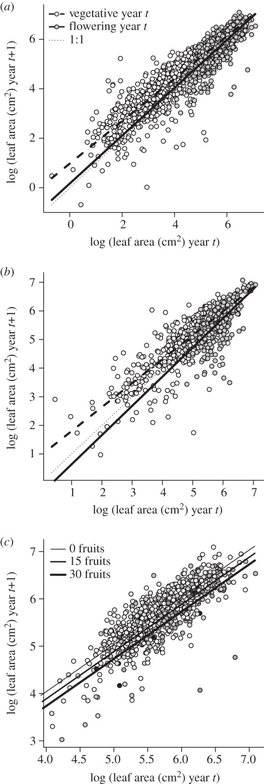
The IPM for O. purpurea consists of plants that vary continuously in size (N(x)) plus three discrete stages: protocorms (P), tubers (T) and dormant plants (D). The continuous component of the IPM consists of demographic functions that predict growth (γ(y, x)), probability of survival (σ(x)), probability of flowering (β(x)), number of flowers produced (ϕ(x)) and probability of dormancy (μ(x)), based on size (x), the natural logarithm of total leaf area, log_e (cm²). The growth function γ(y, x) predicts growth from size x to y. Together, the demographic functions characterize all possible transitions from size in one year (x) to size in the next (y), and they are dynamically linked to the discrete components of the population as follows. Protocorm production is estimated as the number of flowers produced per plant in the previous year multiplied by the proportion of flowers that set fruit (υ), the number of seeds per fruit (α) and the seed-to-protocorm transition probability (ε), integrated over the range of plant sizes (Ω):

2.1

Protocorms that survive (probability σ_P) become tubers the following year:

2.2

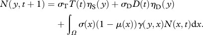
Tubers that survive (probability σ_T) recruit into the continuous size distribution the following year as seedlings, following a normal distribution of seedling sizes: 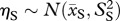. Dormant plants that survive (probability σ_D) also recruit into the continuous size distribution the following year, following a different normal distribution of sizes: 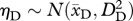. We do not include the possibility of dormancy for more than 1 year (this was observed only twice). Growth from size x to y is conditioned on the probabilities of surviving and not going dormant. Thus, continuous size dynamics are given by:

2.3

Finally, the dynamics of dormant plants are given by:

2.4

(c). Parameter estimation and detection of reproductive costs

We estimated parameters of the continuous demographic functions with generalized linear mixed effects models using the appropriate error distribution (Gaussian for growth; binomial for survival, flowering and dormancy; Poisson for number of flowers). Year was included as a random effect in all models, which were fitted in R v. 2.13.0 using the ‘lmer()’ function [41]. Demographic functions were fit separately for the light and shade environments, as previous work indicated strong differences between habitats [37,40]. Including site within habitat rarely improved the fits of the demographic functions, and so we pooled data between the two sites in each habitat. We lacked habitat-specific estimates of the number of seeds per fruit (α) and the seed-to-protocorm transition (ε), so these were assumed to be constant across habitats. Also, because dormancy was rare, we pooled data from the light and shade environments to better estimate the size distribution of plants emerging from dormancy.

To quantify costs of reproduction, we asked whether including information about reproduction in year t − τ improved prediction of growth (γ), survival (σ) and dormancy (μ) in year t + 1. Because negative demographic effects of reproduction by perennial plants may be time-lagged [42], we tested for lags of τ = 0 (no lag), 1 and 2 years. We decomposed costs of reproduction into the cost of producing a flowering stalk and the cost of producing a fruit, given that a plant has flowered. For each demographic process, we compared four candidate models in which flowering status in year t − τ, a categorical explanatory variable (vegetative or flowering), modified the intercept of the function, the slope of the function (with respect to size), both or neither (null model). We further asked whether increasing fruit production imposed additional costs, beyond the cost of flowering per se. Using the data for flowering plants only, we fitted the same four candidate models as above with number of fruits produced in year t − τ as the predictor variable. We used Akaike's information criterion (AIC) to evaluate each set of candidate models. We took a conservative approach and only rejected the null model (no cost of reproduction) if an alternative model reduced the AIC value by more than two units [43]. We repeated this procedure for each value of τ to determine how far back in an individual's reproductive history we needed to consider in the construction of the O. purpurea IPM.

The results of these analyses were used to account for growth, survival and/or dormancy costs of reproduction in the component functions of the IPM. Because we found no evidence for lagged costs of reproduction (§3), we present remaining methods assuming τ = 0. For demographic functions that differed between vegetative (V) and flowering (F) plants, we accounted for this difference by weighting the two functions by the probability of flowering:

2.5

where f represents the growth, survival or dormancy functions. Any additional reproductive costs are included in f_F with an explicit term for fruits (ϕ(x)υ). It is through these modifications that the demographic model ‘perceives’ the cost of reproduction. Note that if flowering were fatal (σ_F(x) = 0), the IPM would reduce to a semelparous model. Thus, we recover the popular semelparous model as a special case of this more general life-history model.

Our approach to quantifying reproductive costs involves several assumptions. First, we assume that reproduction directly affects only growth, survival and/or dormancy, and that any effect of current reproduction on future reproduction occurs indirectly via these processes. Previous work in this system [40] documented negative associations between flowering in year t and the probability of flowering in year t + 1. However, flowering also reduced growth or caused shrinkage (§3), and accounting for this growth difference explains the association between flowering and subsequent flowering (for both habitats, additional coefficients for previous flowering are not statistically significant in models relating current size and current flowering probability). Second, our model considers only the female component of fitness. Finally, predicting optimal life-history strategies requires that we provide the model with information not only about the costs incurred by plants that reproduce, but also the costs that would be incurred if plants that do not reproduce did. The continuous nature of the component functions of the IPM allows us to do this by linearly extrapolating the demographic performance of reproductive plants into regions of the size distribution where plants were not observed to reproduce. Previous studies have used similar approaches [44]. Thus, we assume that realized costs of reproduction provide accurate information about potential costs of reproduction.

(d). Life-history optimization

We used the fully parametrized IPM for each light environment to calculate optimal reproductive parameters, given the observed demographic context and reproductive costs. We estimated a fitness surface over a range of reproductive parameters and compared observed reproductive strategies with those that are expected to maximize fitness. We used as a fitness proxy the net reproductive rate, R₀. Under certain assumptions (below), parameter combinations that yield the maximum R₀ represent the optimal or ES life history. Thus, we assume genetic variation in and heritability of reproductive parameters. We optimized reproductive parameters separately for the light and shade habitats. To implement the IPM, we discretized the continuous component of the life cycle into 100 bins, which provided sufficient resolution for convergence of model output. R₀ was calculated following Ellner & Rees [7].

The use of R₀ as a fitness proxy is valid for constant environments as long as any density dependence operates at the establishment stages of the life cycle (i.e. limitation of regeneration sites and not antagonistic interactions among established individuals) [45]. We tested the assumption that density dependence operates at the establishment stages by examining the relationship between population-level seed production and seedling recruitment [8,16]. Because the first 3 years of development occur below ground, we tested for correlations between total seed production and seedling recruitment 3 years later, separately, for each of the two study sites in each light environment. Seedlings’ recruitment was not correlated with population-level seed production in any site or light environment (light 1: r = −0.16, t₄ = −0.34, p < 0.7; light 2: r = −0.5, t₃ = −1.0, p < 0.4; shade 1: r = 0.69, t₄ = 1.9, p < 0.15; shade 2: r = 0.002, t₄ = 0.006, p < 0.9), consistent with the assumption that density dependence acts during establishment.

The details of our optimization procedure were data-driven, following the model selection results. In both the light and shade habitats, where we detected costs of flowering (§3), we optimized R₀ over the intercept (β₀) of the flowering function β(x), holding all other parameters at their observed values. Optimizing over both the intercept and slope (β₁) results in a step function, indicating a sharp size threshold for reproduction. The step function is generally regarded as unrealistic, as many factors can maintain variation in size at flowering, and so we focus on the intercept, following previous studies [10,18]. The median size at the onset of reproduction can be calculated as –β₀/β₁; a more negative intercept corresponds to a larger median size at reproduction, and hence a longer delay. We tested for habitat differences in ES flowering size by generating 10 000 bootstrap replicates of our full dataset in which the habitat (light or shade) was randomly shuffled among observations of inter-annual transitions. We estimated the ES β₀ in each habitat from each bootstrap replicate and compared the actual difference between habitats with the 5th and 95th percentiles of the distribution of differences expected owing to chance.

In addition, in the light environment, we detected an additional cost of each fruit produced (§3). Therefore, for the light habitat model, we also optimized R₀ simultaneously over both the intercept and slope of the function for size-dependent flower production ϕ(x), holding other parameters at their observed values. Together, the parameters of ϕ(x) determine the number of flowers produced at a given size and the degree to which flower production increases with size. Note that fruit production is linearly related to flower production by the fruit set parameter υ. We did not optimize over υ because fruit set was shown to be limited by pollination [46] and is therefore not expected to be under selection owing to costs of reproduction.

3. Results

(a). Parameter estimation and detection of reproductive costs

We found evidence for costs of reproduction manifested in the year immediately following reproduction (τ = 0) but not in subsequent years (electronic supplementary material, table S1). Therefore, we do not further consider time lags (τ ≥ 1) in the demographic costs of reproduction. First, reproductive status of plants in year t (vegetative or flowering) significantly modified growth from t to t + 1 in both light and shade habitats by influencing both the intercept and slope of the growth function (table 1 and figure 1). The growth cost of reproduction was greater for smaller plants. In the light habitat, vegetative and flowering plants experienced positive growth, on average, across the size distribution, though vegetative plants were predicted to have a growth advantage, especially when small (figure 1a). In the shade habitat, the fitted growth cost of reproduction was more severe: plants that flowered when small were predicted to shrink in size, while vegetative plants were predicted to grow (figure 1b). Vegetative plants occupied a broader range of the size distribution than reproductive plants in both habitats. Yet their growth differences persisted even when we restricted the analyses to regions of overlap (not shown). Thus, the strong evidence for growth costs of reproduction is not driven by the disparity in size representation.

Table 1.

Model selection analyses for the detection of costs of reproduction for growth, survival and dormancy. Bold values indicate the lowest AIC. ΔAIC gives the AIC difference between each model and the minimum of the set, and AIC weight gives the proportional weight of evidence in favour of each.

demographic function	type of cost	parameter affected	light habitat		shade habitat
			ΔAIC	AIC weight	ΔAIC	AIC weight
growth	cost of flowering	none	56.0	<0.0001	54.0	<0.0001
		intercept	5.0	0.075	2.0	0.26
		slope	18.0	<0.0001	10.0	0.005
		intercept and slope	0	0.92	0	0.73
	cost per fruit	none	7.2	0.02	0	0.99
		intercept	0	0.86	9.8	0.01
		slope	4.0	0.12	13.4	<0.0001
		intercept and slope	11.0	<0.0001	18.2	<0.0001
survival	cost of flowering	none	2.3	0.12	1.8	0.24
		intercept	0.4	0.32	3.7	0.092
		slope	0	0.39	3.8	0.087
		intercept and slope	1.6	0.17	0	0.58
dormancy	cost of flowering	none	0	0.43	0	0.39
		intercept	1.2	0.23	0.9	0.25
		slope	1.1	0.25	0.8	0.26
		intercept and slope	3.0	0.095	2.8	0.097

Figure 1.

(a,b) Observed (points) and fitted (thick lines) patterns of growth from year t to t + 1 for plants that were vegetative (white points, dashed line) or flowering (grey points, solid line) in year t. Thin dotted line represents size stasis. (a) Light habitat, (b) shade habitat. (c) Growth of flowering plants in the light habitat in relation to the number of fruits produced in year t. Darker points indicate greater fruit production (min.: 0, max.: 27). Lines show the fitted growth function at three levels of fruit production.

In the light environment, we detected an additional growth penalty for each fruit produced (table 1). This penalty modified only the intercept of the growth function for flowering plants. Thus, the fitted effect of fruit production on growth is irrespective of size (figure 1c).

In contrast to growth, no single survival model received unambiguous support from the demographic data (table 1). However, most of the mortality occurred among small vegetative plants that had not yet started flowering (figure 2a,b). For example, we observed a total of 72 and 31 mortality events in the light and shade habitats, respectively; of these, 64 and 28 occurred at sizes below the flowering threshold. Thus, there was little information with which to extrapolate the survival costs of flowering for small plants. When we restricted the analyses to size ranges in which both vegetative and flowering plants were represented, support for the null model (no reproductive cost) increased in both habitats. Therefore, we took a conservative approach and used the null model (black lines in figure 2a,b) in the O. purpurea IPM. For comparison, we also show the functions with the lowest AIC values (grey lines in figure 2a,b). Survival was greater in the light habitat than in the shade habitat, especially for small plants.

Figure 2.

(a,b) Size-dependent survival and (c,d) dormancy in (a,c) light and (b,d) shade habitats. Points show binned proportions for plants that were vegetative (white circles) or flowering (grey circles) in year t. Thick black lines show the fitted null models. Thin grey lines in (a,b) show the best-fit model that incorporates differences between vegetative (dashed) and flowering (solid) plants (note that these differences are driven by the concentration of mortality at pre-reproductive sizes).

Finally, the probability of dormancy was best described by size-dependent functions without reproductive costs in both habitats (table 1). Dormancy probability increased with size but was low, occurring in only 1.2 per cent of our inter-annual observations. Because we could not distinguish immediate mortality from mortality during dormancy, we set dormant plant survival (σ_D) as 1.0 in both habitats.

The fitted growth, survival and dormancy functions, and all other demographic parameters are given in electronic supplementary material, table S2. The asymptotic population growth rates (λ) were 1.091 in the light habitat and 1.002 in the shade habitat, in agreement with previous results from these populations [40].

(b). Optimization of demographic parameters

(i). Probability of flowering, β(x)

The observed growth costs of reproduction (figure 1) favoured reproductive delay in both light and shade habitats (figure 3). Optimization of R₀ over the intercept of the flowering function (holding the flower production function ϕ(x) at the estimated parameters) allowed us to characterize selection on the duration of delay (size at flowering). In both habitats, the cost of reproduction led to strong fitness peaks for the intercept of the flowering function, and hence median reproductive size. By contrast, when we removed the growth cost of reproduction (all plants grew like vegetative plants), selection favoured the smallest possible size at flowering (figure 3, dashed lines). The optimal size at reproduction was smaller in the light habitat than in the shade habitat (table 2), consistent with the greater growth cost of flowering (figure 1) and mortality risk (figure 2) in the shade. However, the observed difference in ES β₀ values between habitats (0.77) fell within the 5th and 95th percentiles of the null distribution (−2.52, 1.92).

Figure 3.

Optimal and observed flowering strategies in (a) light and (b) shade habitats. Strategies are represented as the value of the intercept of the flowering function, β(x), which determines the median reproductive size. Solid lines show the fitness landscapes incorporating observed growth costs of reproduction. Dashed lines show the fitness landscapes without any costs. In the light habitat, dotted lines show the fitness landscape including the cost of flowering but not the per-fruit growth penalty. Black dots indicate the fitness peaks. Vertical lines indicate values estimated from the demographic data and the grey regions represent the 95% confidence intervals (±2 s.d.). Fitness values (R₀) were transformed to relative fitness by dividing by the maximum.

Table 2.

Predicted and observed flowering strategies in each habitat. (Values in parentheses following the observed intercepts are the upper and lower bounds of the 95% confidence intervals on the parameter estimates.)

	light	shade
predicted intercept of flowering function β(x)	−18.37	−17.60
observed intercept of flowering function β(x)	−18.64 (−20.25, −17.03)	−17.93 (−20.29, −15.57)
predicted median flowering size (log(cm2))	4.99	5.61
observed median flowering size (log(cm2))	5.06	5.71

The predicted reproductive delay in the shade environment was driven entirely by the growth cost of flowering, as this was the only cost we detected and included in the IPM. However, in the light environment, both the cost of flowering and the per-fruit growth penalty contributed to selection on size at flowering. We quantified the contribution of the additional cost by optimizing R₀ with the per-fruit cost set to zero, which led to a slightly smaller optimal flowering size (figure 3a, dotted lines).

We compared the optimal values for the intercept of the flowering function with values that were independently estimated from the demographic data (electronic supplementary material, table S1). There was remarkable consistency between observed and ES reproductive strategies in both habitats (figure 3 and table 2). In the light environment, the per-fruit growth penalty, in addition to the cost of flowering, was necessary to account for the observed flowering strategy (figure 3). The CI on the intercept of the flowering functions largely overlapped for the light and shade habitats (table 2). Still, the estimated median flowering size was 11 per cent larger in the light habitat, in agreement with the 11 per cent difference in fitness-maximizing strategies between habitats (table 2).

(ii). Flower production, ϕ(x)

In the light environment, optimizing R₀ over the intercept and slope of the flower production function (holding the flowering function β(x) at the estimated parameters) resulted in a fitness surface with a ridge instead of a peak (figure 4). This indicates that costs of reproduction select for a particular relationship between the slope and intercept, but many possible combinations could satisfy this relationship. The parameter combination estimated from the demographic data (black rectangle in figure 4) falls far from the ridge of maximum fitness. The difference between optimal and observed values translates to an orders-of-magnitude difference in flower production. For example, the fitted parameters predict a mean of 33.5 flowers per plant at the observed median reproductive size, whereas a similarly sized plant on the ridge of maximum fitness would produce approximately 1000 flowers.

Figure 4.

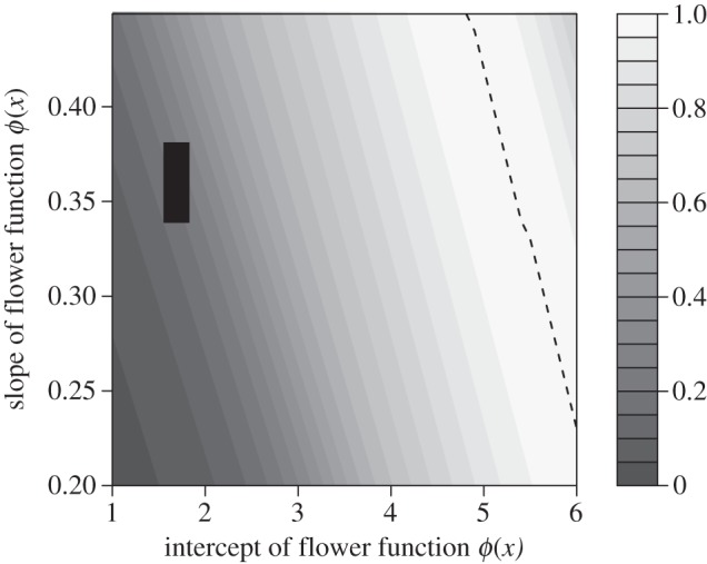
Optimal and observed strategies for flower production in the light habitat. The surface represents relative fitness (lighter is greater) in relation to the intercept and slope of the size-dependent flower production function, ϕ(x). Dashed line indicates the ridge of maximum fitness. Black rectangle shows the joint 95% confidence region (±2 s.d.) of the parameters estimated from the demographic data.

4. Discussion

Understanding why organisms delay reproduction is a long-standing puzzle in evolutionary ecology that has most often been investigated in the context of semelparous life histories. We have shown that non-lethal costs of reproduction in an iteroparous species select for delayed reproduction. Flowering and fruit production by O. purpurea were associated with reduced growth and the cost of flowering was size-dependent: the smaller the plant, the greater the reduction in growth. We did not find strong evidence for a direct effect of reproduction on mortality or dormancy. Rather, reproduction indirectly reduced survival because it retarded gains in size (and even caused shrinkage to smaller size), and mortality risk was greater for smaller plants. Reproduction also indirectly reduced future reproductive output because flowering probability and flower production were size-dependent. Together, these factors selected for a cautious life history that includes a prolonged reproductive delay (a new O. purpurea recruit would require 4–5 years to reach the observed reproductive size). A similar combination of size-dependent costs and size-dependent demography is thought to shape the reproductive strategy of ungulates [26].

That costs of reproduction favour the evolution of reproductive delay is not particularly surprising. What is surprising about our results is just how accurately the costs that we estimated were able to account for observed reproductive delays. Predicted and estimated values for the intercept of the flowering function (which determines median reproductive size) were remarkably consistent in both habitats. The difference between habitats in optimal flowering strategy, while not statistically significant, was consistent in direction with other demographic differences: the growth cost of flowering was more severe—causing shrinkage to a smaller size, on average—and the size-dependent risk of mortality was greater in the shade versus the light habitat. Combined, these factors appear to select for a larger reproductive size in the shade (and hence a longer delay). However, the statistical overlap of observed reproductive strategies in the light and shade habitats provides no strong evidence for responses to habitat-specific selection.

While we found a near-perfect match between optimal and observed flowering size, there was significant disagreement between optimal and observed parameters for the size-dependent flower production function in the light environment. A plant behaving ‘optimally’ would produce many more flowers, given their size, than real plants do. This discrepancy could be attributed to several factors. First, we may have under-estimated the fruit cost. A sensitivity analysis indicated that increasing the fruit cost above the levels we estimated would bring optimal parameter combinations closer to observed values, especially if pollen limitation was weaker (electronic supplementary material). Second, flower production is likely to be under constraints that are not related to reproductive costs. Most optimization approaches to life-history evolution, including ours, are blind to the morphologies in which demographic parameters are packaged. Plant architecture and allometric relationships are strongly influenced by phylogenetic history. That making 1000 flowers would confer an orchid with greater lifetime fitness is beside the point; it simply cannot make 1000 flowers because it is an orchid. The relevant question is whether costs of flowering or fruit production cause plants to deviate from what their phylogenetic and architectural limits might otherwise allow. For O. purpurea, there is not yet a clear answer. The development of quantitative methods that accommodate both the costs of reproduction and the constraints on reproduction is an important frontier in our understanding of iteroparous reproductive strategies.

Consideration of temporal variation in the environment is another important future direction in the study of iteroparous life histories. For example, it has been shown for semelparous plants that the direction and magnitude of selection on flowering size can vary from year to year [8] and that covariance between demographic rates could amplify the effects of stochasticity [14]. Our qualitative conclusions regarding the importance of non-lethal costs in selecting for delayed reproduction are probably robust to our assumption of environmental constancy, as stochasticity alone does not favour reproductive delay when adult survival exceeds juvenile survival [22], as was the case for O. purpurea (figure 2). However, temporal variation could influence the quantitative details of ES reproductive strategies. Understanding this influence is important, particularly in the face of non-stationary environmental variability associated with climate change.

A persistent challenge in the study of iteroparous life histories is the difficulty in detecting and characterizing costs of reproduction. In contrast to semelparous plants, in which the cost of reproduction is self-evident, documenting reproductive costs in iteroparous plants requires looking for them, and costs are sometimes elusive. This is particularly true for observational datasets, where costs may be masked by or confounded with genetic or environmental factors [25]. For this reason, others have advocated experimental manipulations of reproductive effort [31,34,42,47,48] and we agree that more experimental studies are needed. Even when costs can be detected from observational datasets, experiments would be useful for validating observational patterns, as negative correlations between demographic parameters do not necessarily reflect trade-offs [49], and positive correlations are often predominant [50]. Nearly all experiments to date have decreased reproductive output (e.g. by removing flowering stalks or flower buds)—an obvious and straightforward type of manipulation. Our study, like some previous ones [51], highlights the importance of the hypothetical cost of reproduction that would be paid by individuals smaller than the current reproductive size threshold. Experimental efforts to induce flowering at typically vegetative sizes, possibly using hormones, would be extremely valuable for validating the extrapolation approach employed here.

In summary, the combination of long-term demographic data and continuously size-structured models has generated novel insights into the selective forces that shape reproductive strategies. Our study highlights the ways in which methods developed for the study of semelparous life histories can be generalized to iteroparous organisms. Given that the majority of plants are iteroparous [52], we expect that our approach will be broadly applicable. These methods can also be applied to iteroparous animals with size-structured demography, including vertebrates, marine invertebrates and social insect colonies. The relative complexity of iteroparous life histories poses important challenges (e.g. quantifying the strength and form of reproductive costs), but also rich opportunities for testing theories of life-history evolution. This is particularly important given the potential influence of ongoing environmental change, which could not only modify the distribution and abundance of populations but also select on the life-history strategies of individuals.

References

- 1.Hard J. J., Gross M. R., Heino M., Hilborn R., Kope R. G., Law R., Reynolds J. D. 2008. Evolutionary consequences of fishing and their implications for salmon. Evol. Appl. 1, 388–408 10.1111/j.1752-4571.2008.00020.x (doi:10.1111/j.1752-4571.2008.00020.x) [DOI] [PMC free article] [PubMed] [Google Scholar]
- 2.Kuparinen A., Merilä J. 2007. Detecting and managing fisheries-induced evolution. Trends Ecol. Evol. 22, 652–659 10.1016/j.tree.2007.08.011 (doi:10.1016/j.tree.2007.08.011) [DOI] [PubMed] [Google Scholar]
- 3.Bell G. 1980. The costs of reproduction and their consequences. Am. Nat. 116, 45–76 10.1086/283611 (doi:10.1086/283611) [DOI] [Google Scholar]
- 4.Stearns S. C. 1992. The evolution of life histories. Oxford, UK: Oxford University Press [Google Scholar]
- 5.Metcalf C. J. E., Rose K. E., Rees M. 2003. Evolutionary demography of monocarpic perennials. Trends Ecol. Evol. 18, 471–480 10.1016/S0169-5347(03)00162-9 (doi:10.1016/S0169-5347(03)00162-9) [DOI] [Google Scholar]
- 6.Easterling M. R., Ellner S. P., Dixon P. M. 2000. Size-specific sensitivity: applying a new structured population model. Ecology 81, 694–708 10.1890/0012-9658(2000)081[0694:SSSAAN]2.0.CO;2 (doi:10.1890/0012-9658(2000)081[0694:SSSAAN]2.0.CO;2) [DOI] [Google Scholar]
- 7.Ellner S. P., Rees M. 2006. Integral projection models for species with complex demography. Am. Nat. 167, 410–428 10.1086/499438 (doi:10.1086/499438) [DOI] [PubMed] [Google Scholar]
- 8.Childs D. Z., Rees M., Rose K. E., Grubb P. J., Ellner S. P. 2004. Evolution of size-dependent flowering in a variable environment: construction and analysis of a stochastic integral projection model. Proc. R. Soc. Lond. B 271, 425–434 10.1098/rspb.2003.2597 (doi:10.1098/rspb.2003.2597) [DOI] [PMC free article] [PubMed] [Google Scholar]
- 9.de Jong T. J., Klinkhamer P. G. L., Prins A. H. 1986. Flowering behaviour of the monocarpic perennial Cynoglossum officinale, L. New Phytol. 103, 219–229 10.1111/j.1469-8137.1986.tb00610.x (doi:10.1111/j.1469-8137.1986.tb00610.x) [DOI] [PubMed] [Google Scholar]
- 10.Hesse E., Rees M., Muller-Scharer H. 2008. Life-history variation in contrasting habitats: flowering decisions in a clonal perennial herb (Veratrum album). Am. Nat. 172, E196–E213 10.1086/591683 (doi:10.1086/591683) [DOI] [PubMed] [Google Scholar]
- 11.Kachi N., Hirose T. 1985. Population dynamics of Oenothera glazioviana in a sand-dune system with special reference to the adaptive significance of size-dependent reproduction. J. Ecol. 73, 887–901 10.2307/2260155 (doi:10.2307/2260155) [DOI] [Google Scholar]
- 12.Kuss P., Rees M., Ægisdottir H. H., Ellner S. P., Stöcklin J. 2008. Evolutionary demography of long-lived monocarpic perennials: a time-lagged integral projection model. J. Ecol. 96, 821–832 10.1111/j.1365-2745.2008.01374.x (doi:10.1111/j.1365-2745.2008.01374.x) [DOI] [Google Scholar]
- 13.Metcalf C. J. E., Rees M., Buckley Y. M., Sheppard A. W. 2009. Seed predators and the evolutionarily stable flowering strategy in the invasive plant, Carduus nutans. Evol. Ecol. 23, 893–906 10.1007/s10682-008-9279-8 (doi:10.1007/s10682-008-9279-8) [DOI] [Google Scholar]
- 14.Rees M., Childs D. Z., Metcalf C. J. E., Rose K. E., Sheppard A. W., Grubb P. J. 2006. Seed dormancy and delayed flowering in monocarpic plants: selective interactions in a stochastic environment. Am. Nat. 168, E53–E71 10.1086/505762 (doi:10.1086/505762) [DOI] [PubMed] [Google Scholar]
- 15.Rees M., Rose K. E. 2002. Evolution of flowering strategies in Oenothera glazioviana: an integral projection model approach. Proc. R. Soc. Lond. B 269, 1509–1515 10.1098/rspb.2002.2037 (doi:10.1098/rspb.2002.2037) [DOI] [PMC free article] [PubMed] [Google Scholar]
- 16.Rose K. E., Louda S. M., Rees M. 2005. Demographic and evolutionary impacts of native and invasive insect herbivores: a case study with Platte thistle, Cirsium canescens. Ecology 86, 453–465 10.1890/03-0697 (doi:10.1890/03-0697) [DOI] [Google Scholar]
- 17.Wesselingh R. A., Klinkhamer P. G. L., De Jong T. J., Boorman L. A. 1997. Threshold size for flowering in different habitats: effects on size-dependent growth and survival. Ecology 78, 2118–2132 [Google Scholar]
- 18.Williams J. L. 2009. Flowering life-history strategies differ between the native and introduced ranges of a monocarpic perennial. Am. Nat. 174, 660–672 10.1086/605999 (doi:10.1086/605999) [DOI] [PubMed] [Google Scholar]
- 19.Metcalf C. J. E., Rose K. E., Childs D. Z., Sheppard A. W., Grubb P. J., Rees M. 2008. Evolution of flowering decisions in a stochastic, density-dependent environment. Proc. Natl Acad. Sci. USA 105, 10 466–10 470 10.1073/pnas.0800777105 (doi:10.1073/pnas.0800777105) [DOI] [PMC free article] [PubMed] [Google Scholar]
- 20.Hautekeete N.-C., Piquot Y., Van Dijk H. 2002. Life span in Beta vulgaris ssp. maritima: the effect of age at first reproduction and disturbance. J. Ecol. 90, 508–516 [Google Scholar]
- 21.Tuljapurkar S. 1990. Delayed reproduction and fitness in variable environments. Proc. Natl Acad. Sci. USA 87, 1139–1143 10.1073/pnas.87.3.1139 (doi:10.1073/pnas.87.3.1139) [DOI] [PMC free article] [PubMed] [Google Scholar]
- 22.Koons D. N., Metcalf C. J. E., Tuljapurkar S. 2008. Evolution of delayed reproduction in uncertain environments: a life-history perspective. Am. Nat. 172, 797–805 10.1086/592867 (doi:10.1086/592867) [DOI] [PubMed] [Google Scholar]
- 23.Calow P. 1989. The cost of reproduction: a physiological approach. Biol. Rev. Camb. Phil. Soc. 54, 32–40 [DOI] [PubMed] [Google Scholar]
- 24.Harper J. L. 1977. The population biology of plants. New York, NY: Academic Press [Google Scholar]
- 25.Obeso J. R. 2002. The costs of reproduction in plants. New Phytol. 155, 321–348 10.1046/j.1469-8137.2002.00477.x (doi:10.1046/j.1469-8137.2002.00477.x) [DOI] [PubMed] [Google Scholar]
- 26.Proaktor G., Coulson T., Milner-Gulland E. J. 2008. The demographic consequences of the cost of reproduction in ungulates. Ecology 89, 2604–2611 10.1890/07-0833.1 (doi:10.1890/07-0833.1) [DOI] [PubMed] [Google Scholar]
- 27.Miller T. E. X., Tenhumberg B., Louda S. M. 2008. Herbivore-mediated ecological costs of reproduction shape the life history of an iteroparous plant. Am. Nat. 171, 141–149 10.1086/524961 (doi:10.1086/524961) [DOI] [PubMed] [Google Scholar]
- 28.Ackerman J. D., Montalvo A. M. 1990. Short- and long-term limitations to fruit production in a tropical orchid. Ecology 74, 263–272 10.2307/1940265 (doi:10.2307/1940265) [DOI] [Google Scholar]
- 29.Calvo R. N. 1993. Evolutionary demography of orchids: intensity and frequency of pollination and the cost of fruiting. Ecology 74, 1033–1042 10.2307/1940473 (doi:10.2307/1940473) [DOI] [Google Scholar]
- 30.Pfeifer M., Heinrich W., Jetschke G. 2006. Climate, size and flowering history determine flowering pattern of an orchid. Bot. J. Linn. Soc. 151, 511–526 10.1111/j.1095-8339.2006.00539.x (doi:10.1111/j.1095-8339.2006.00539.x) [DOI] [Google Scholar]
- 31.Primack R. B., Hall P. 1990. Costs of reproduction in the pink lady's slipper orchid: a four-year experimental study. Am. Nat. 136, 638–656 10.1086/285120 (doi:10.1086/285120) [DOI] [PubMed] [Google Scholar]
- 32.Shefferson R. P., Proper J., Beissinger S. R., Simms E. L. 2003. Life history trade-offs in a rare orchid: the costs of flowering, dormancy, and sprouting. Ecology 84, 1199–1206 10.1890/0012-9658(2003)084[1199:LHTIAR]2.0.CO;2 (doi:10.1890/0012-9658(2003)084[1199:LHTIAR]2.0.CO;2) [DOI] [Google Scholar]
- 33.Shefferson R. P., Simms E. L. 2007. Costs and benefits of fruiting to future reproduction in two dormancy-prone orchids. J. Ecol. 95, 865–875 10.1111/j.1365-2745.2007.01263.x (doi:10.1111/j.1365-2745.2007.01263.x) [DOI] [Google Scholar]
- 34.Sletvold N., Ågren J. 2011. Among-population variation in costs of reproduction in the long-lived orchid Gymnadenia conopsea: an experimental study. Oecologia 167, 461–468 10.1007/s00442-011-2006-0 (doi:10.1007/s00442-011-2006-0) [DOI] [PMC free article] [PubMed] [Google Scholar]
- 35.Visser M. D., Jongejans E., van Breugel M., Zuidema P. A., Chen Y.-Y., Kassim A. R., de Kroon H. 2011. Strict mast fruiting for a tropical dipterocarp tree: a demographic cost–benefit analysis of delayed reproduction and seed predation. J. Ecol. 99, 1033–1044 10.1111/j.1365-2745.2011.01825.x (doi:10.1111/j.1365-2745.2011.01825.x) [DOI] [Google Scholar]
- 36.Rose F. 1948. Flora of the British Isles. Orchis purpurea Huds. J. Ecol. 36, 366–377 10.2307/2256683 (doi:10.2307/2256683) [DOI] [Google Scholar]
- 37.Jacquemyn H., Brys R., Jongejans E. 2010. Seed limitation restricts population growth in shaded populations of a perennial woodland orchid. Ecology 91, 119–129 10.1890/08-2321.1 (doi:10.1890/08-2321.1) [DOI] [PubMed] [Google Scholar]
- 38.Jacquemyn H., Brys R. 2010. Temporal and spatial variation in flower and fruit production in a food-deceptive orchid: a five-year study. Plant Biol. 12, 145–153 10.1111/j.1438-8677.2009.00217.x (doi:10.1111/j.1438-8677.2009.00217.x) [DOI] [PubMed] [Google Scholar]
- 39.Jacquemyn H., Brys R., Honnay O. 2009. Large population sizes mitigate negative effects of variable weather conditions on fruit set in two spring woodland orchids. Biol. Lett. 5, 495–498 10.1098/rsbl.2009.0262 (doi:10.1098/rsbl.2009.0262) [DOI] [PMC free article] [PubMed] [Google Scholar]
- 40.Jacquemyn H., Brys R., Jongejans E. 2010. Size-dependent flowering and costs of reproduction affect population dynamics in a tuberous perennial woodland orchid. J. Ecol. 98, 1204–1215 10.1111/j.1365-2745.2010.01697.x (doi:10.1111/j.1365-2745.2010.01697.x) [DOI] [PubMed] [Google Scholar]
- 41.R Core Development Team 2011. R: A language and environment for statistical computing. Vienna, Austria: R Foundation for Statistical Computing: See http://www.R-project.org [Google Scholar]
- 42.Ehrlén J., van Groenendael J. 2001. Storage and the delayed costs of reproduction in the understorey perennial Lathyrus vernus. J. Ecol. 89, 237–246 10.1046/j.1365-2745.2001.00546.x (doi:10.1046/j.1365-2745.2001.00546.x) [DOI] [Google Scholar]
- 43.Burnham K. P., Anderson D. R. 2002. Model selection and multimodel inference: a practical information-theoretic approach, 2nd edn New York, NY: Springer [Google Scholar]
- 44.Roff D. A. 1983. An allocation model of growth and reproduction in fish. Can. J. Fish. Aquat. Sci. 40, 1395–1404 10.1139/f83-161 (doi:10.1139/f83-161) [DOI] [Google Scholar]
- 45.Mylius S. D., Diekmann O. 1995. On evolutionarily stable life histories, optimization and the need to be specific about density dependence. Oikos 74, 218–224 10.2307/3545651 (doi:10.2307/3545651) [DOI] [Google Scholar]
- 46.Jacquemyn H., Brys R., Hermy M. 2002. Flower and fruit production in small populations of Orchis purpurea Huds. and implications for management. In Trends and fluctuations and underlying mechanisms in terrestrial orchid populations (eds Kindlmann P., Willems J., Whigham D. F.). Kerkwerve, The Netherlands: Backhuys [Google Scholar]
- 47.Koivula M., Koskela E., Mappes T., Oksanen T. A. 2003. Cost of reproduction in the wild: manipulation of reproductive effort in the bank vole. Ecology 84, 398–405 10.1890/0012-9658(2003)084[0398:CORITW]2.0.CO;2 (doi:10.1890/0012-9658(2003)084[0398:CORITW]2.0.CO;2) [DOI] [Google Scholar]
- 48.Hartemink M., Jongejans E., de Kroon H. 2004. Flexible life history responses to flower and rosette bud removal in three perennial herbs. Oikos 105, 159–167 10.1111/j.0030-1299.2004.12784.x (doi:10.1111/j.0030-1299.2004.12784.x) [DOI] [Google Scholar]
- 49.Knops J. M. H., Koenig W. D., Carmen W. J. 2007. Negative correlation does not imply a tradeoff between growth and reproduction in California oaks. Proc. Natl Acad. Sci. USA 104, 16 982–16 985 10.1073/pnas.0704251104 (doi:10.1073/pnas.0704251104) [DOI] [PMC free article] [PubMed] [Google Scholar]
- 50.Jongejans E., de Kroon H., Tuljapurkar S., Shea K. 2011. Plant populations track rather than buffer climate fluctuations. Ecol. Lett. 13, 736–743 10.1111/j.1461-0248.2010.01470.x (doi:10.1111/j.1461-0248.2010.01470.x) [DOI] [PubMed] [Google Scholar]
- 51.Roff D. A. 1986. Predicting body size with life history models. Bioscience 36, 316–323 10.2307/1310236 (doi:10.2307/1310236) [DOI] [Google Scholar]
- 52.Hart R. 1977. Why are biennials so few? Am. Nat. 111, 792–799 10.1086/283209 (doi:10.1086/283209) [DOI] [Google Scholar]