Predicting oscillatory dynamics in the movement of territorial animals

Abstract

Understanding ecological processes relies upon the knowledge of the dynamics of each individual component. In the context of animal population ecology, the way animals move and interact is of fundamental importance in explaining a variety of observed patterns. Here, we present a theoretical investigation on the movement dynamics of interacting scent-marking animals. We study how the movement statistics of territorial animals is responsible for the appearance of damped oscillations in the mean square displacement (MSD) of the animals. This non-monotonicity is shown to depend on one dimensionless parameter, given by the ratio of the correlation distance between successive steps to the size of the territory. As that parameter increases, the time dependence of the animal's MSD displays a transition from monotonic, characteristic of Brownian walks, to non-monotonic, characteristic of highly correlated walks. The results presented here represent a novel way of determining the degree of persistence in animal movement processes within confined regions.

1. Introduction

To secure a habitat to forage and successfully reproduce, many animals display territorial behaviour by excluding intruders from certain regions of space [1]. Depending on the species, territorial defence is accomplished in different modalities. One such modality, which is common to most terrestrial mammals, is scent-marking [2]. By depositing scent, an animal ensures that its presence is broadcast to other individuals, as scent marks, in particular, the non-volatile components may persist in the environment and be perceived as ‘fresh’ for prolonged periods. Within that period, the so-called active scent time, animals need to refresh their own scent to maintain an exclusive use of their territories [3]. When a conspecific encounters a foreign active scent mark at a given location, it recognizes that location is claimed by another animal. To avert potential costly confrontation, an intruder responds by avoiding the areas where ‘fresh’ foreign scent is present. When residents and intruders belong to the same species, this response mechanism is called conspecific avoidance. A recent theoretical study, validated with experimental observations on urban foxes, has elucidated the role of conspecific avoidance and scent-mediated interaction in the collective formation of territorial patterns [4]. The study has shown that conspecific avoidance at the level of the individual generates an exclusion process [5] at the level of the territories, making it apparent that territoriality is a complex emergent phenomenon.

Since territories are exclusive, their dynamics are subdiffusive and much slower than the movement rate of an animal [4]. This disparity in movement rates has made possible the construction of analytical expressions describing animals moving within slowly fluctuating territories [6], as well as a model representation of the fine-scale dynamics of interacting territorial boundaries [7]. In the above studies [6,7], the analysis was limited to one dimension and, more importantly, the assumption had been that an animal moves as a Brownian walker. Although the representation of animal movement via the diffusive hypothesis has been used since the 1950s [8], there exist other more general representations of movement statistics that reduce to the Brownian case under appropriate limits. Two such examples are correlated random walks [9–12] and Lévy walks [13,14]. Whereas the former has a long mathematical history [15], the latter has been proposed more recently [16] and only in the last decade has it been used as a tool to analyse and interpret animal movement data [17–19]; however, its use has not been immune to criticisms [20–25]. Here, we are interested in exploring the dynamics of a territorial animal in two dimensions when its movement possesses some degree of persistence.

Compared with a Brownian walker, a correlated random walker possesses directional persistence, which is well suited for animals moving within a familiar confined area such as a territory. After some initial wandering within its own territory, an animal acquires a good knowledge of its environment. Subsequent movements owing to foraging needs or for border patrolling are more likely directed towards well-known locations, introducing a persistence in the movement statistics. A correlated random walk gives a good phenomenological representation of such persistence, as the movement is the result of short displacement distances and a selection of turning angles from a distribution peaked around zero, which controls the degree of bias of the walk [10]. In one dimension, the continuum limit of a random walk governed by such a bias (only 0 and ±π ‘turning angles’ are possible) has been shown to result in a probability distribution function satisfying a telegrapher's equation [15]. In dimensions higher than one, although no continuum limit can be found that reduces a persistent random walk exactly to the corresponding higher dimensional telegrapher's equation [26,27], such an equation interpolates between a wave equation and a diffusion equation, that is between ballistic and Brownian motion. We exploit this feature to study the effects of persistence in the movement statistics of territorial animals by using a telegrapher's equation within confined space. We obtain approximate analytical solutions that represent a territorial animal moving with a variable degree of correlation. We analyse the validity of the analytical results by comparing them to stochastic simulations of many interacting scent-marking animals that move as correlated random walkers. We predict the appearance in certain conditions of damped oscillations in the animal's mean square displacement (MSD), if the underlying movement is that of a highly correlated random walker, whereas no oscillatory dynamics exist if territorial animals move as Brownian walkers.

2. Model

The starting point of the analysis is the reduction of the non-Markovian problem of moving and scent-marking animals to that of a single moving animal within slowly fluctuating boundaries. Owing to territorial exclusion, there is a time-scale disparity between the movement of the animals, which are diffusive, and the movement of the territorial boundaries, which are subdiffusive, giving rise to an MSD long-time dependence that increases in two dimensions proportional to t/ln(t) [4] as function of time t, the expected result in two-dimensional exclusion dynamics [28]. To find an approximate expression and reduce the dimensionality of the problem, it is necessary to make a type of mean-field approximation, as adopted in Giuggioli et al. [6], and consider one individual animal moving within a territory whose boundary shape may fluctuate but whose area is forced around a value equal to the inverse of the population density. We describe this forcing by connecting the boundaries with effective springs. These spring-like dynamics of the territory size represent two competing effects: the acquisition of new territory by the resident animal and the neighbours' pressure for territorial takeover. This approximation is represented pictorially in figure 1.

Figure 1.

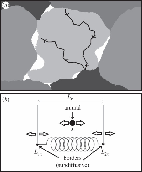
(a) Pictorial representation of the territorial random walk model, and (b) its mean-field approximation. (a) Each shade denotes the area where a particular animal has deposited fresh scent (its territory). The white areas are interstitial regions, where there is no fresh scent from any animal. Territory borders move when an animal travels into the interstitial region and leaves scent cues, thus claiming the region for its own territory. A territory's size will tend to fluctuate around an average value equal to the inverse of the population density. The black line denotes a possible path of an animal inhabiting the light grey territory. Panel (b) shows a schematic of the reduced analytical model, displayed in one dimension for diagrammatic simplicity. The borders move randomly and subdiffusively, but are joined together by a spring whose rest distance is the average territory width. In two dimensions, the average territory size corresponds to a rest ‘area’ enclosed by two springs along two orthogonal axes, whose dimension is the inverse of the population density. For circular geometry, the territory radius fluctuates around a rest distance that encloses an area whose dimension is the inverse of the population density. The parameters controlling the animal movement vary between the ballistic and the Brownian limit. In between those two extremes, an animal moves with some degree of persistence, e.g. as a correlated random walker.

In the reduced model dynamics, the mathematical description is given by the joint probability distribution P(X, L,t) of having an animal at location X and the boundaries described by L, which represents either the four-dimensional Cartesian coordinates for rectangular territories or the three-dimensional vector for circular territories with two coordinates related to the territorial centroid position and one to the radius of the territory. Furthermore, since the boundary locations move very little during the time scale over which the walker diffuses, one can invoke an adiabatic approximation [6] and consider the joint probability distribution as P(X, L, t) ≈ Q(L, t)W(r, t|L), with Q(L, t) being the probability distribution of the boundaries' location and W(r, t|L) the probability distribution of the animal position for a given L. This decoupling allows us to treat separately the dynamics of the boundaries from that of the walker. The boundary dynamics are governed by a Fokker–Planck equation (see equation (A 1) in appendix A) with a time-dependent diffusion coefficient. The presence of this time dependence ensures that the MSD is not that owing to Brownian statistics, but rather is subdiffusive owing to territorial exclusion. The specific functional dependence of φ(t) is dictated by the expected and observed territorial boundary MSD at long times.

2.1. The boundaries

In Cartesian coordinates, the probability distribution for the boundaries being at locations L at time t is simply the product of the probability distribution along each axis. We have in fact that Q(L, t) = Q_x(L_1x, L_2x, t)Q_y(L_1y, L_2y, t) with Q_σ(L_1σ, L_2σ, t) given by (see appendix A)

2.1

where λ_σ = L_2σ–L_1σ is the separation distance between the right and left boundary along the positive direction of the σ axis, ℒ_σ = (L_2σ + L_1σ)/2 is the centroid of the boundary locations along σ, b_σ(t) = 4(K_σ/γ_σ){1 − exp[−2γ_σ ∫₀^t dsφ(s)]}, c_σ(t) = 2K_σ∫₀^t dsφ(s), and H(y) is the Heaviside function such that H(y) = 1 if y > 0 and H(y) = 0 if y < 0. Notice that the presence of the Heaviside function and the sum of two Gaussians centred at ±L_σ are the result of having required the separation distance between two boundaries to be always positive. The rate at which territorial boundaries return to their average distance is represented through γ_σ, and the slow dynamics of the boundaries is due to the time-dependent diffusion constant φ(t), which governs how the Gaussian spreads over time through the MSD of a single boundary as a function of time, given by the term ∫₀^t dsφ(s). If φ(t) is independent of time, the variance of the Gaussian distributions increases linearly with time, and the dynamics of the boundaries is diffusive, whereas for a time-dependent φ(t), the diffusion becomes anomalous.

For circular territories, we consider fluctuations both for the centroid location and the radial extent of the territory. To take into account the subdiffusive nature of the fluctuations, the probability distribution for the centroid coordinates (x_c,y_c) and the radius ρ of the territory satisfy a Fokker–Planck equation with a time-dependent diffusion coefficient (see appendix A), whose solution is given by

2.2

where and . Analogous to the rectangular territories, the dependence on the sum of two Gaussians in the variable ρ is because ρ ≥ 0 and the presence of a time dependence in φ(t) makes the boundary dynamics anomalous.

2.2. The animal

For the animal, we represent the degree of persistence in its two-dimensional walk as it moves within a confined area through the two parameters of the telegrapher's equation: the speed v and the time constant T. This time constant is related to the time spent by an animal moving along a straight line without turning. It has been shown that such a random walker can be described in the continuum limit by a radially symmetric two-dimensional telegrapher's equation augmented by an inhomogeneous term [27,29]. This inhomogeneous term decays exponentially to zero at a rate proportional to T⁻¹. For our purpose, we neglect this term and we describe approximately the animal persistence through a telegrapher's equation with reflecting boundary conditions at the territorial boundaries.

In Cartesian coordinates, the animal probability distribution W(r, t|L) for a given location L of the boundaries is simply the product of each probability distribution along each axis and it satisfies the telegrapher's equation along each σ-axis, that is

2.3

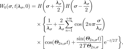
The analytical solution of equation (2.3) along each axis with reflecting boundaries (see appendix B) can be expressed as the infinite series

2.4

written here for the simple case in which the boundary centroid is the origin. The subscript 0 for W in equation (2.4) indicates that the initial position of the animal is the origin and the Θ_n,σ parameters are given by

2.5

For animals moving within circular territories, we write the two-dimensional telegrapher's equation in polar coordinates as

2.6

where, similarly to the Cartesian case, T is the average time for which a walker keeps moving before changing direction and v is the animal speed. The solution of equation (2.6) with reflecting boundary conditions at the territory boundaries can be computed exactly (see appendix B) giving the result

2.7

where

2.8

and with μ_nm the mth zero of the derivative of the nth Bessel function of the first kind J_n(z), i.e. the values of μ satisfied by the implicit equation [30].

The ballistic regime in equations (2.4) and (2.7) is obtained by taking the limit T →+∞, whereas the diffusive regime is obtained by taking the limits T → 0 and v →+∞ such that v²T = D with D representing the animal diffusion constant. With the latter procedure in the Cartesian case 2TΘ_n,σ → 1 and the time dependence in the series reduces to , whose first-order expansion in T gives exp[−(2n)²π²Dt/λ_σ²], thus recovering the one-dimensional expression reported in equation (C1) of Giuggioli et al. [6]. For the polar case, in the diffusive limits, the time dependence exp[−t/(2T)][cos(tΩ_0m) + sin(tΩ_0m)/(2TΩ_0m)] simplifies to exp(−μ_0m²Dt/ρ²) and equation (2.7) becomes the probability distribution of a Brownian walker confined in a circular domain of radius ρ reported in Polyanin [31]. These limiting procedures, in both Cartesian and polar geometries, are also valid in the more general case, reported in appendix B in equations (B 10) and (B 22), of off-centre initial conditions and off-centre location of the territory centroid.

3. Results

In exploring the parameter dependence of the animal MSD, it is convenient to start analysing the simpler situation corresponding to when territories are immobile, that is the boundary diffusion constant K = 0, which corresponds to when the active scent time of a territorial animal is infinitely large. We thus study first the time dependence of the animal MSD for immobile boundaries in §3.1, whereas the case with fluctuating boundaries is dealt with in §3.2.

3.1. Damped oscillatory dependence of the animal mean square displacement with immobile boundaries

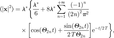
The general expression for the animal MSD in rectangular confinement has been written explicitly in equation (C 1) in appendix C. The square geometry is a simplification of the rectangular geometry and can be easily derived from equation (C1) by considering λ_x = λ_y = λ*. When the animal initial condition and the centroid of the territory are placed at the origin, the MSD expression in an immobile square territory of length λ* centred at the origin is equal to

3.1

where the symbol 〈···〉 represents an ensemble average, that is, an average over the associated probability distribution. At short times, the time-dependent term [cos(Θ_nt) + sin(Θ_nt)/(2TΘ_n)]exp[−t/(2T)] reduces to 1 − t²n²π²v²/(2λ*²) giving a short time increase equal to 2v²t² (see appendix C for details).

In an immobile circular territory with initial conditions centred at the origin, the MSD in equation (C4) reduces to

3.2

which can be shown (see appendix C) to have the appropriate 2v²t² short time dependence.

The exponential term exp[−t/(2T)] present in the convergent series of equations (3.1) and (3.2) ensures that at long times, the MSD saturates to a constant value since each element of the series becomes identically zero. An inspection of equations (3.1) and (3.2) shows that the animal MSD may display oscillatory behaviour in time when the quantities Θ_n or Ω_0m, defined, respectively, in equations (2.5) and (2.8), are real. For a given dimensionless parameter ζ = vT/λ* or ξ = vT/ρ, the suppression of the oscillatory dependence owing to the cosine and sine terms of the series in equation (3.1) or (3.2) increases as n or m gets larger. As a result, the terms of the series that contribute the most to the oscillations are the smallest n and m that makes Θ_n or Ω_0m real, which occurs, respectively, when ζ > (4π)⁻¹ ≃ 0.08 and when ξ > (2μ₀₁)⁻¹ ≃ 0.13. These estimates are very close to the transition values of ζ and ξ beyond which non-monotonicity appears, determined numerically by plotting the MSD in figures 2 and 3 for, respectively, the square and circular geometry (see captions of the figures). The Matlab code to plot the analytical expressions (3.1) and (3.2) can be found in the electronic supplementary material.

Figure 2.

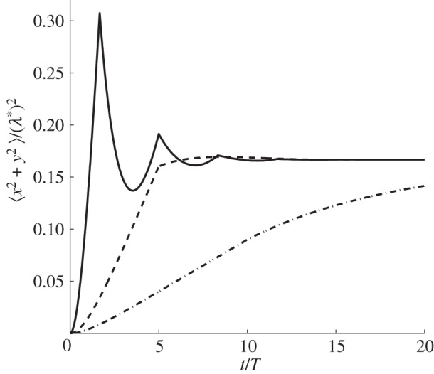
Mean square displacement (MSD) of an animal with varying amount of directional persistence in immobile square boundaries. Depending on the value of the parameter ζ = vT/λ*, by plotting equation (3.1), it is possible to observe three qualitatively different time dependencies. For ζ < 0.086, the MSD appears monotonic, whereas it displays non-monotonicity for ζ ≥ 0.086. We distinguish two types of non-monotonicity depending on the number of maxima above the value at which the MSD saturates. When only one maximum is visible, using a numerical precision of 10⁻⁴, we name the time dependence as over-damped. If more than two or more maxima are visible, we name the time dependence as under-damped. Study of the parameter space shows that when 0.086 ≤ ζ < 0.102, the dynamics are over-damped, whereas they are under-damped when ζ ≥ 0.102. Solid line, ζ = 0.3; dashed line, ζ = 0.1; dash-dotted line, ζ = 0.05.

Figure 3.

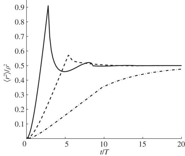
MSD of an animal with varying amount of directional persistence in immobile circular boundaries. Depending on the value of the parameter ξ = vT/ρ, by plotting equation (3.2), it is possible to observe three qualitatively different time dependencies. For ξ < 0.12, the MSD appears monotonic, whereas it displays non-monotonicity for ξ ≥ 0.12. By using the same definition for under- and over-damped dynamics as in figure 2, we notice that when 0.12 ≤ ξ < 0.20, the time dependence is over-damped, whereas it is under-damped when ξ ≥ 0.20. Solid line, ξ = 0.35; dashed line, ξ = 0.18; dash-dotted line, ξ = 0.1.

The appearance of a non-monotonic dependence in the MSD as well as the eventual saturation have an intuitive explanation. The parameters ζ and ξ represent the average distance an animal would travel without turning (the term vT) relative to the characteristic length λ* of the available space in the square geometry and the radius ρ in the circular case. In the extreme case, when ζ or ξ are infinitely large, the movement becomes ballistic and the walker, starting at the origin, would always return to the origin infinitely many times. With ζ or ξ sufficiently large but finite, the chance that a trajectory would not return to the origin would increase over time, progressively reducing the height of the maxima in the MSD. Eventually, the movement would become diffusive and the probability of finding the walker anywhere in the territory would become constant. Similar reasoning applies when the animals start off-centre, although the nature of the periodicity when ζ or ξ are infinitely large is owing to the movement paths being like billiard trajectories [32].

A peculiar characteristic, which is evident from the MSD plots, is the presence of very sharp maxima in the underdamped regime for sufficiently large values of ζ and ξ. This feature can be readily explained in the Cartesian case as follows. When ζ is in the underdamped regime, when n is sufficiently large and the series in equation (3.1) can be written as . The dominant contribution in this infinite series comes from the cosine terms, which displays maxima at t/T = (k + 1/2)/ζ with k = 0, 1, 2, … . These values correspond to the locations of the sharp maxima in figure 2. To understand the presence of the apparent discontinuous derivative of the MSD at the maxima, one needs to differentiate the cosine series above and realize that , which indeed has discontinuous jumps at t/T = (k + 1/2)/ζ with k = 0, 1, 2, … . A similar argument helps explain the appearance of sharp peaks in the circular case. When ξ is in the underdamped regime, when m is sufficiently large and the series in equation (3.2) can be approximated by . For large m, one may approximate [30] as well as the Bessel function for large values of its argument and rewrite the series as . This series can be recast in terms of combination of Lerchphi function [33] and shown to possess the first discontinuous derivative at t/T = ξ⁻¹. We have tested numerically that indeed the location of the first maximum in the MSD follows this inverse proportionality relation as function of ξ, with greater accuracy as we increase ξ. Sharp troughs also seem to appear whenever t/T = kξ⁻¹ with k odd, which are precisely the non-smooth points of , as long as k is small enough to be in the oscillatory regime.

3.2. Damped oscillatory dependence of the animal mean square displacement with fluctuating boundaries

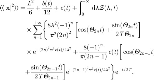
When territorial boundaries fluctuate, the evaluation of the animal MSD requires integration over all possible values of the boundary locations, equivalently over all possible values of the boundary separation λ_σ and territorial centroid ℒ_σ. For the square geometry and when the initial territory centroid and animal position are at the origin, one obtains (see appendix C)

3.3

where the symbol 〈〈···〉〉 signifies that the average is taken both over all possible animal locations as well as territory size and locations, and with 2exp[−(λ² + L²)/b(t)]cosh[2λL/b(t)]/ defined from equation (2.1), and valid for either of the two orthogonal directions.

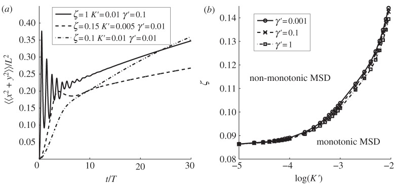
Aside from the actual value of the diffusion constant and spring constant present in b(t), the boundary movement is controlled by the time dependence in φ(t). As animal territories undergo exclusion [4], we select φ(t) = [ln(1 + t/β)]⁻¹ − [ln(1 + t/β)]⁻²(t/β)(1 + t/β)⁻¹ with β being a characteristic time. This choice causes the MSD of the boundary to be , which is an increasing function of time, starting at zero when t = 0 and having the same long-time dependence as objects undergoing exclusion in two dimensions [28]. With this version of φ(t), we plot in figure 4 the MSD dynamics for different parameters, namely K′ = KT/L², γ′ = γT and ζ. Since the size of the territory is now changing, ζ = vT/L represents the average distance moved without turning relative to the average territory length L.

Figure 4.

MSD of a walker starting at the origin inside a square territory with fluctuating boundaries. (a) The MSD as it varies with time for three different values of ζ = vT/L. As ζ increases, we move from a regime where the MSD is monotonic to one where oscillations occur. (b) The ζ values separating the monotonic (upper region) from the non-montonic (lower region) regime, for various choices of the dimensionless parameters K′ = KT/L² and γ′ = γT. The various plots have been constructed using equation (3.3).

Similarly, for the circular geometry, one can define the quantity in equation (2.2) and write, when the initial conditions for the animal and the territory centre are at the origin, the animal MSD as

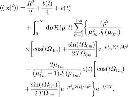3.4

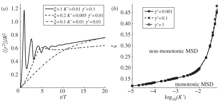
With the earlier-described choice of φ(t), we plot the MSD dynamics for different parameters in figure 5, namely K′ = KT/ρ², γ′ = γT and ξ = vT/R, where R is the average territory radius.

Figure 5.

MSD of a walker starting at the origin inside a circular territory with fluctuating boundaries. (a) The MSD as it varies with time for three different values of ξ = vT/R. As ξ increases, we move from a regime where the MSD is monotonic to one where oscillations occur. (b) The threshold ξ values for passing from one regime into another, for different choices of the dimensionless parameters K′ = KT/ρ² and γ′ = γT. The various plots have been constructed using equation (3.4).

From figures 4 and 5, one feature becomes evident. As ζ or ξ diminishes, the walker becomes more and more Brownian and monotonicity disappears. A comparison between the immobile and the mobile boundary case shows that the oscillations are also observable when boundaries move slowly, as in the case considered here of subdiffusing boundaries. We have wondered therefore if the non-monotonic MSD would still be present if the statistics of the boundary movement were to have an MSD that increases superlinearly. Although this may not be of direct relevance to territorial animals, since territorial boundaries subdiffuse, we have examined whether the analytical model still displays oscillations when the rate of the boundary movement becomes comparable to or larger than that of the walker. For this purpose, we have selected a time-dependent diffusion constant φ(t) ∝ t^η−1 with 1 ≤ η < 2 and with different values of ζ and ξ. It turns out that oscillations always appear when ζ or ξ are sufficiently larger than K′. The Matlab code to plot the analytical expressions (3.3) and (3.4) can be found in the electronic supplementary material.

4. Comparison with stochastic simulations of territorial correlated random walkers

To compare the analytical predictions of the previous sections to the many-bodied system of territorial correlated random walkers, we generalize the territorial random walk model in Giuggioli et al. [4], so that animals move as correlated random walkers rather than diffusive walkers. We implement stochastic simulations of N animals whereby each animal moves as a correlated random walker inside a square terrain of side S with periodic boundary conditions. Step lengths are sampled from an exponential distribution with mean step-length a and turning angles sampled from a wrapped double exponential (Laplace) distribution. In order to model the scent depositing and conspecific avoidance, the terrain contains an underlying grid of smaller squares of side a, where S/a is an integer. Upon landing on a square, a walker marks it with its own scent. This square then becomes part of the walker's territory. The scent remains active for a time T_AS and, in addition to the described movement process, no walker is allowed to move into a square that contains active scent of another walker. Although the territory shape differs from animal to animal, most of the territories acquire more of a round rather than a square shape. It is natural then to compare the stochastic simulations with the results obtained for the circular geometry by determining the value ξ = vT/R. A correlated random walker possesses a correlation time τ related to the turning angle distribution f(θ) via the relation [34] τ = −1/ln[〈cos(θ)〉], where . The average time for which an animal moves without turning in the simulation is thus T = τa/v. R is taken as the mean radius of a territory assuming that territories are circular and have an average size S²/N. We can thus report the output of the simulation as function of ξ.

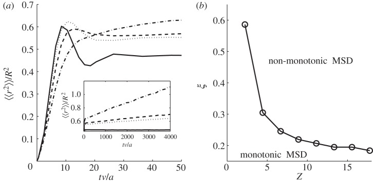
The fundamental dimensionless parameter that characterizes the territorial random walk system is Z = T_ASvaN/S², where v is the velocity of a single walker. Previous work in one dimension [4,6] has shown that the relative rate of displacement of a territory boundary compared with that of an animal is solely controlled by the parameter Z. We thus study the dynamics of the MSD of a territorial random walker by varying not only ξ but also Z as well. The results are plotted in figure 6 showing a non-monotonic MSD when both ξ and Z are sufficiently large. Compared with figure 5, the shape of the curve in figure 6b, separating the monotonic from the non-monotonic regime in parameter space, appears to be inversely proportional. This does not come as a surprise because preliminary results for Brownian walkers have determined that the diffusion constant of the boundaries, here called K_crw because the walkers are correlated, decreases exponentially with Z [4]. In one dimension, this exponential dependence has been shown to arise from a similar exponential dependence in the probability of a territory to extend into interstitial range, as opposed to shrinking further [7]. In turn, this probability turns out to be related to the first passage time for an animal to cross its territory and thus extend it, where possible, into previously interstitial area [7].

Figure 6.

(a) How the MSD varies with time for various different values of Z and ξ. The solid line has ξ = 1.51, Z = 15.56; the dotted line ξ = 1.51, Z = 2.22; the dashed line ξ = 0.80, Z = 2.22; the dot-dashed line ξ = 0.34, Z = 2.22. Before beginning to measure the animal MSD, the simulation was run until such a time as the borders have an MSD proportional to t/ln(t) and each animal was placed in the centre of its territory. This mirrors the initial conditions used in figure 5. In the region where the MSD is non-monotonic, the higher we make both Z and ξ, the more pronounced the oscillatory behaviour. The inset demonstrates the long-time behaviour of the MSD, which is to increase proportional to K_crwt/ln(t), where K_crw depends on both Z and ξ. For the Z = 15.56 case, K_crw is so low that the line looks flat, since K_crw decreases exponentially as Z increases. (b) The threshold value of ξ for various Z, below which the MSD is monotonic and above which it is not.

The inset in figure 6a has been plotted to show that the solid curve, corresponding to large Z and ξ values, appears close to constant, whereas the other curves show a clear increase at long times. Although we would expect that an increase in ξ would generate damped oscillations in the MSD, as ξ becomes too large, the animals move so quickly that they are on average able to re-mark all or most of their territory boundaries before the scent decays away. In such a scenario, the territories move much less. As a consequence, there is no set of parameters for which we obtain a strongly oscillating MSD at intermediate times and a rapidly increasing MSD at long times.

5. Conclusions

We have considered the dynamics of territorial animals that deposit scent in each of the locations they visit. As scent marks persist for some time even in the absence of the signaller, an animal is able to broadcast to other individuals where it has been in the recent past, and thus claim a certain region of space as its own. Quantifying the dynamics of such a system via interacting random walkers is complicated by the intrinsic non-Markovian nature of the processes. In that respect, approximate models of such dynamics become useful for data comparison and predictions. Here, we have explored a two-dimensional one-body reduction of the original many-body problem and we have compared two animal movement statistics, Brownian and correlated random walks. By focusing at intermediate time scales, we predict the appearance of damped oscillations in the animal MSD in certain regimes. Stochastic simulations of territorial correlated random walkers have confirmed that non-monotonicity may appear as the distribution of turning angles is sufficiently narrow, or alternatively as the correlation time is sufficiently large.

Damped oscillatory MSD dynamics owing to confinement and correlations of a generic random process have been predicted in granular materials in terms of the stress variance as function of depth [35] and observed in the context of charged balls constrained to move in a circular channel [36]. Here, we predict damped oscillations in the context of moving animals as function of the movement characteristics and the size of the confining region. Although non-monotonic MSDs appear not to have been observed in the animal kingdom yet, this may simply be owing to such processes being ignored as noise. Furthermore, we believe that future spatio-temporally resolved experimental data will be routinely interpreted through models such as this one since highly accurate tracking devices, e.g. GPS collars, are becoming cheaper and more widespread. As the precision of these devices increases, it is important to consider types of model where the movement statistics are of different kinds. In that respect, we plan to extend this model to situations where animals move as Lévy [13] or self-avoiding walkers [37] as well as other forms of anomalous diffusion [38].

Our theoretical investigations extend previous studies on the characterization of correlations in animal movement data [34,39] to scenarios for which an animal is observed within a confined space. This is clearly important since the reconstruction of a turning angle distribution from the observed animal trajectory would include the turns owing to the boundaries of the available space. In such a scenario, it becomes more appropriate to interpret the data in terms of a correlation distance or a correlation time, which does not include the turns associated with the reflections at boundaries. These quantities are precisely the parameters vT and T, respectively, of our telegrapher's equation model. The value of T may then be related to the persistence of the animal in an unbounded domain via the mean cosine of the distribution of turning angles [34].

Furthermore, the appearance or otherwise of oscillations in the MSD may allow one to discern more easily the processes underlying movement data, when data have been collected with a relatively long sampling rate. In such a case, examining turning angles between fixes could result in the movement looking Brownian when the process is in fact correlated. However, the appearance of oscillations in the MSD could help discern whether the walk is correlated in this scenario, without needing to gather further finer-grained movement data.

Since the period of oscillations is approximately equal to vT²/L in square territories and directly related to vT²/R in circular territories, a measurement of the speed and turning angles when the animal is unaffected by foreign scent boundaries may provide a novel methodology to estimate the dimensions of a territory. The presence of sharp maxima (square territories) as well as sharp minima (circular territories) in the oscillations may also help in the actual model fitting of experimental observations. In summary, besides the obvious applicability to the dynamics of territorial animals, our study provides a useful quantitative tool to characterize animal movement in confined space and offers the opportunity to differentiate between plausible interpretations of the underlying movement statistics.

Appendix A. Probability distribution of the randomly fluctuating boundaries

A.1. Rectangular territories

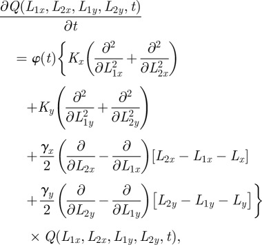
To describe the time dependence of the probability distribution Q(L,t) of the fluctuating boundary positions L = (L_2x, L_1x, L_2y, L_1y) along the x and y coordinates, we use the two-dimensional Fokker–Planck equation

A1

where φ(t) is the dimensionless time-dependent diffusion, K is the boundary diffusion constant, γ represents the rate with which the separation between territory boundaries returns to the value L_σ per unit length squared, and L_σ is the average separation distance between the right and left boundaries along the σ-axis. Equation (A 1) is the extension in two dimensions of the approximate model used to study the dynamics of one dimension territorial walkers [6].

When φ(t) is time-independent, equation (A 1) reduces to a diffusive process for the four boundary locations along the σ axes (σ = x or σ = y). The separation distance along each axis is also a random Gaussian process. When φ(t) is time-dependent, represents a Gaussian random process whose probability broadens in time along each of the four components proportionally to [6,40]. To ensure that always remains positive, equation (A 1) needs to be supplemented by the boundary conditions . For a generic φ(t), one can solve equation (A 1) with the above-mentioned boundary condition through separation of variables [6] by seeking solutions of the partial differential equation of the form . For initial conditions of the type , with δ(z) a Dirac delta function, that is, if and , equation (A 1), when initially , is exactly solved by the expression reported in equation (2.1) of the main text.

A.2. Circular territories

For animal territories of circular rather than rectangular shape, we construct a Fokker–Planck equation for the boundary, which is equivalent to (A 1). In Cartesian coordinates, the fluctuations of the boundaries are decomposed into a centroid location and a separation term. In keeping with this analogy, the probability distribution is defined in terms of a centroid with coordinates (x_c, y_c) and a radial extent of the territory ρ. A spring force constrains the radial variations to be around the value R and the subdiffusive nature of the fluctuations are taken into account with the time-dependent function φ(t), giving a Fokker–Planck equation of the form

A2

Equation (A 3) is supplemented with the boundary condition because ρ must remain positive at all times. Similar to the case of rectangular territories, the presence of the time-dependent diffusion constant φ(t) that multiplies the right-hand side of the equation describes a Gaussian process whose time dependence is subordinated to φ(t). The functional dependence of φ(t) is chosen in such a way that the boundary MSD reproduces the observed long-time behaviour of the MSD in the territorial random walk system. Equation (A 3) is decomposable along each direction and thus one can straightforwardly write the solution as the product of the dynamics for the territory radius and the territory centroid. For localized initial conditions of the type Q(x_c, y_c, ρ, 0) = δ(ρ − R)δ(x_c)δ(y_c), the exact analytical solution has been reported in equation (2.2) of the main text.

Appendix B. Probability distribution of the randomly moving animal

B.1. Cartesian coordinates

Through separation of variables, equation (2.3) with the reflective boundary condition at the territorial boundaries can be solved exactly. The simplest way to proceed is to derive a probability distribution W*(σ, t) for the case when the boundaries are at position −λ/2 and λ/2, where λ is the length of the territory. The final result in equation (B 10) will then be obtained by shifting values of σ and σ₀ by the centroid location. By seeking solutions of the form W*(σ, t) = g(t)q(σ) and substituting in equation (2.3) one can write

B1

and

B2

where α² is a real constant to be defined. The only allowed solutions of equation (B 2) satisfying the boundary condition and normalized to 1 are those for which α² < 0, i.e. if α = i|α| with , giving

B3

The imposition of the boundary conditions dq(x)/dx|_{x =±λ/2} = 0 requires either

or

Equation (B 1) has the general solution , where , with . Further imposing the condition one can write the time dependence as

B4

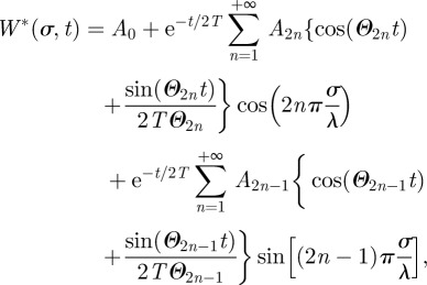
By making a linear superposition of all the possible solutions satisfying the boundary and initial conditions one can write the general solution of W*(σ, t) in the interval −λ/2, λ/2 as

B5

where the constants A_n (containing the term 4TΘ_n/(2TΘ_n − 1)) need to be determined based on the initial condition W*(σ, 0) and the fact that W*(σ, t) is normalized at all times. Normalization makes A₀ = 1/λ, whereas the other A_n constants depend explicitly on the choice of the initial conditions. We will consider in particular the case when W*(σ, 0) = δ(σ − σ₀), where δ is a Dirac delta distribution whose representation in a finite domain can be expressed as

B6

in the limit .

Equation (B 5) is a Fourier series representation of W*(σ, t) and the coefficients A_n can be computed via

and

B7

Using equation (B 6), the Green function becomes

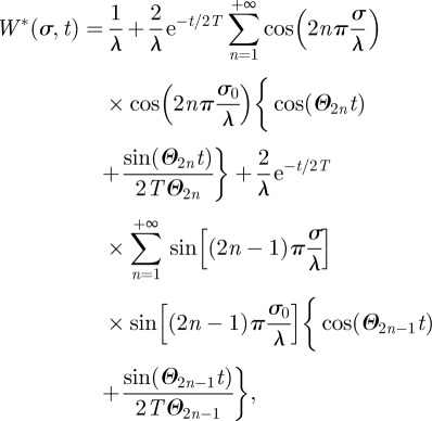B8

which can also be written in the more compact form

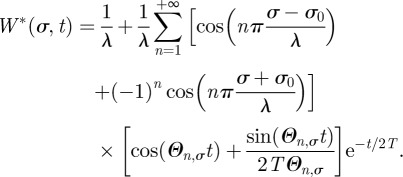B9

By shifting the coordinates σ and σ₀ by the amount equal to −(λ_2σ + λ_1σ)/2 one then obtains

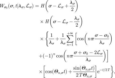B10

with Θ_n,σ defined in equation (2.5) of the main text and where the subscript σ₀ and the symbols λ_σ and ℒ_σ on the left-hand side make explicit the dependence in W on the animal initial position and boundary locations, respectively.

Equation (B 10) when the left boundary is at the origin has been derived in the past in Masoliver et al. [41] and can also be found in Polyanin [31]. The simplified expression when σ₀ = 0 and ℒ_σ = 0 has been reported in equation (2.1) of the main text.

B.2. Polar coordinates

The Green function solution of equation (2.6) with reflective boundary condition at r = ρ can also be found by the method of separation of variables. By seeking solutions of the form W(r, θ, t) = q(r)Θ(θ)g(t), one obtains the equation

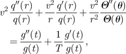B11

and separately solve the equations

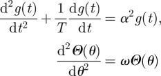and

B12

where the constants α² and ω need to be determined.

Since the probability distribution must be single-valued, we require that . From the general form of the solution in , i.e. one realizes that there exist solutions only if , where n is an integer. We thus have

The radial dependence then becomes

B13

whose solution is

B14

where I_n(z) and K_n(z) are, respectively, modified Bessel functions of order n of the first and second kind [42]. Since the modified Bessel functions are monotonic increasing functions, the only way to satisfy the reflective boundary condition at r = ρ is that α² ≤ 0, i.e. α = i|α|. We thus have that the radial solution is of the form

B15

where J_n(z) is a Bessel function of the first kind and E₂ = 0 since Y_n(z) ∝ K_n(iz) possess a divergence at r = 0. For convenience, one can define now the constant β = α/v whose units are the inverse length. To satisfy the boundary condition , we then require that , which occurs in correspondence of the zeros of the derivative of the Bessel function [30]. We can thus write the general form of the radial solution as

B16

where β_nm is the mth positive zeros of the trascendental equation . If β = 0, then a non-trivial solution is only possible if n = 0 and it gives a constant value. Solution of the time-dependent part follows the same derivation as in the previous section, giving a constant when β = 0, and g(t) = cos(tΩ_nm) + sin(tΩ_nm)/(2TΩ_nm), where now . The linear superposition of all the possible solutions then gives

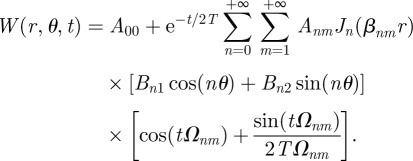B17

To determine the various constants, we first use the fact that W(r, θ, t) is normalized at all times. Computing one reduces the infinite n-series to just the n = 0 term, while all the terms in the m-series are identically zero because . For normalization purposes, we thus have that A₀₀ = 1/(πρ²). For the other constants, we exploit the fact that equation (B 17) is a Bessel series in r, which implies that [30]

for all β ≥ 0 satisfying with δ_p,m a Kronecker delta. Furthermore, since

we obtain

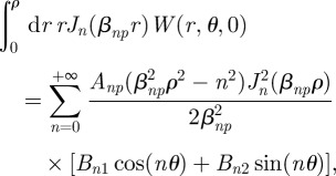which gives us the relation

B18

Analogous to the calculations for the radial variable, one can exploit the fact that equation (B 17) is also a Fourier series in θ. By multiplying equation (B 17) by cos(nθ) and sin(nθ), one gets the n-coefficients of the Fourier series in θ as

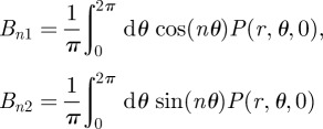B19

For localized initial conditions of the form W(r, θ, 0) = f₁(r)f₂(θ) with

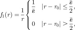B20

in the limit and

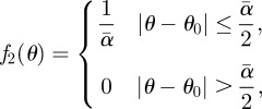B21

in the limit , one obtains the following expression:

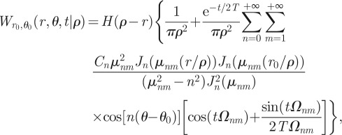B22

where C_n = 1 if n = 0 and C_n = 2 if n ≥ 1, and where the subscript r₀, θ₀ and the symbol ρ make explicit the dependence on, respectively, the initial animal position and the radial extent of the territory. The parameters β_nm in equation (B 17) have been rewritten in equation (B 22) as a dimensionless quantity such that β_nmr, β_nmr₀ and β_nmρ are expressed, respectively, as μ_nmr/ρ, μ_nmr₀/ρ and μ_nm with μ_nm the mth zero of the trascendental equation , and where Ω_nm has been written in equation (2.8) of the main text. Equation (B 22) and its diffusive limit coincides with the expressions reported in Polyanin [31]. With the initial condition r₀ = 0, the expression above reduces to equation (2.7) reported in the main text.

Appendix C. Animal mean square displacement

C.1. Rectangular territories

In rectangular coordinates, the expression for the MSD is obtained by calculating the integral ∫_L1x^L_2x dx ∫_L1yL_2y dy [(x−x₀)²+(y−y₀)²]W(x, y, t|L), where . The resulting expression is given by

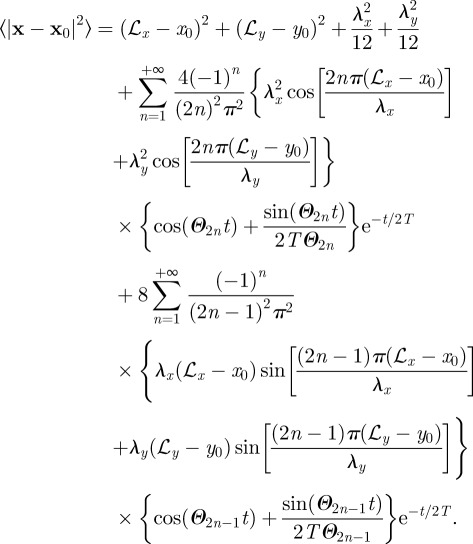C1

At short times, equation (C 1) can be evaluated by noticing that and that for −1/2 ≤ z ≤ 1/2, where z = x₀/λ* or z = y₀/λ*, and . With simple algebra, one can then show that the MSD increases as . The expression in equation (3.1) of the main text is derived from equation (C 1) when the territories are square and centred at the origin with the walker starting from the origin as well.

When territorial boundaries fluctuate, to obtain the animal MSD, one needs to integrate over and along the two directions. For the case of square territories, one first multiplies equation (C 1) by , given in equation (2.1), and then simplifies the resulting expression by setting , , , with L the inverse square root of the population density, and for or y. After integration over the variable ℒ, one can write the animal MSD as

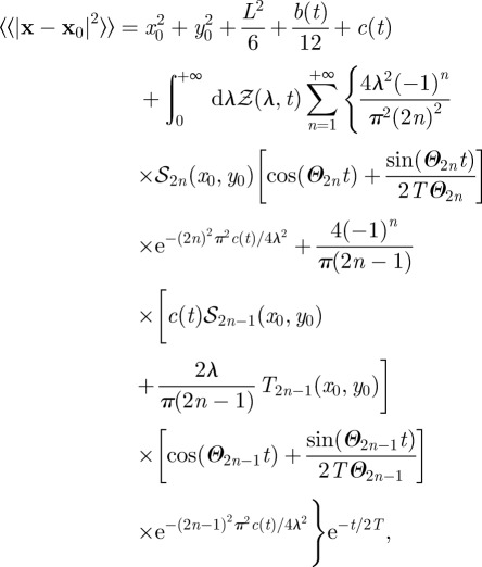C2

wherein has been defined in §3.2 of the main text, and . In the simpler case, when , and and expression (C 2) reduces to equation (3.3), as shown in the main text.

C.2. Circular territories

The calculation of the MSD in polar coordinates is carried forward by realizing that , where r, and , are measured with respect to a chosen origin. Given that and one obtains

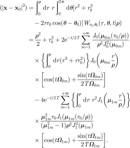C3

By repetitive use of the relations , and , one can show that , , and , thus reducing equation (C 3) to

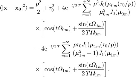Equation (C 4) simplifies to equation (3.2) reported in the main text, when the animal initial condition coincides with the origin. At short times, one has that reduces to . As with Cartesian coordinates, one can now insert the short time expansion and evaluate the series given that [30] and that with . In addition, twice differentiation with respect to z of these two identities allows us to show that, and . With some simple algebra, one then deduces that the MSD in equation (C 4) at short times grows as .

To find the MSD expression when boundaries fluctuate, one first needs to rewrite equation (C 4) with respect to a fixed origin, which we choose as , and obtain the expression

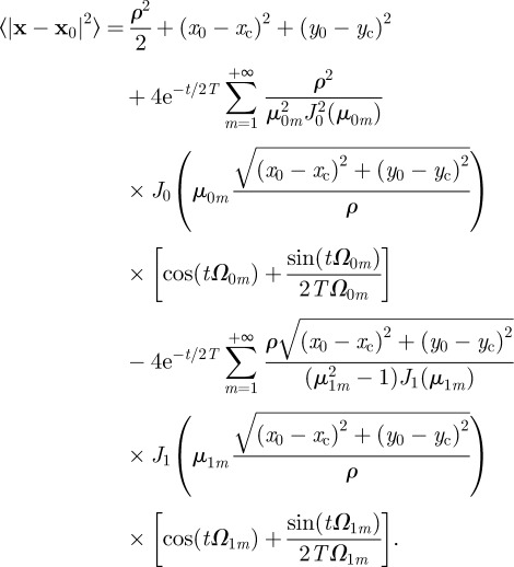To average over all possible territory sizes and territory centroid locations, one needs to multiply equation (C 5) by equation (2.2) and integrate over the lengths , between and and over the length ρ between 0 and . The resulting expression can be simplified by changing the variable of integration for the centroid location from to the shifted polar coordinates and and performing a polar integration in and . By using the shifted polar coordinates, one can rewrite the weighting function in equation (2.2) as where and have been written, respectively, as and . The integration over can now be simplified by recognizing that where is the modified Bessel function of the first kind of order 0. Finally, integrating over both the radius and the length ρ gives the equation

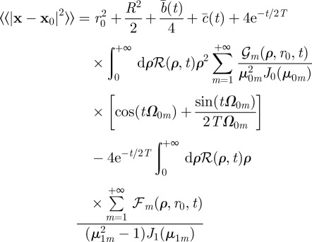where , where , and where has been defined in the main text before equation (3.4). In the simpler case, when and , one obtains the expression (3.4) reported in the main text.

References

- 1.Klopfer P. H. 1969. Habitats and territories; a study of the use of space by animals. New York, NY: Basic Books [Google Scholar]
- 2.Hurst J. L. 2005. Scent marking and social communication. In Animal communication networks (ed. McGregor P. K.), pp. 219–243 Cambridge, UK: Cambridge University Press [Google Scholar]
- 3.Johnson R. P. 1973. Scent marking in mammals. Anim. Behav. 21, 521–535 10.1016/S0003-3472(73)80012-0 (doi:10.1016/S0003-3472(73)80012-0) [DOI] [Google Scholar]
- 4.Giuggioli L., Potts J. R., Harris S. 2011. Animal interactions and the emergence of territoriality. PLoS Comp. Biol. 7, e1002008. 10.1371/journal.pcbi.1002008 (doi:10.1371/journal.pcbi.1002008) [DOI] [PMC free article] [PubMed] [Google Scholar]
- 5.Harris T. E. 1965. Diffusion with ‘collisions’ between particles. J. Appl. Probab. 2, 323–338 10.2307/3212197 (doi:10.2307/3212197) [DOI] [Google Scholar]
- 6.Giuggioli L., Potts J. R., Harris S. 2011. Brownian walkers within subdiffusing territorial boundaries. Phys. Rev. E 83, 061138. 10.1103/PhysRevE.83.061138 (doi:10.1103/PhysRevE.83.061138) [DOI] [PubMed] [Google Scholar]
- 7.Potts J. R., Harris S., Giuggioli L. 2011. An anti-symmetric exclusion process for two particles on an infinite 1D lattice. J. Phys. A 44, 485003. 10.1088/1751-8113/44/48/485003 (doi:10.1088/1751-8113/44/48/485003) [DOI] [Google Scholar]
- 8.Skellam J. G. 1951. Random dispersal in theoretical populations. Biometrika 38, 196–218 [PubMed] [Google Scholar]
- 9.Kareiva P., Shigesada N. 1983. Analyzing insect movement as a correlated random walk. Oecologia 56, 234–238 10.1007/BF00379695 (doi:10.1007/BF00379695) [DOI] [PubMed] [Google Scholar]
- 10.Bovet P., Benhamou S. 1988. Spatial analysis of animals' movements using a correlated random walk model. J. Theor. Biol. 131, 419–433 10.1016/S0022-5193(88)80038-9 (doi:10.1016/S0022-5193(88)80038-9) [DOI] [Google Scholar]
- 11.Turchin P. 1998. Quantitative analysis of movement. Sunderland, MA: Sinauer Press [Google Scholar]
- 12.Okubo A., Levin S. A. 2001. Diffusion and ecological problems: modern perspectives, 2nd edn New York, NY: Springer [Google Scholar]
- 13.Viswanathan G. M., Buldyrev S. V., Havlin S., da Luz M. G. E., Raposo E. P., Stanley H. E. 1999. Optimizing the success of random searches. Nature 401, 911–914 10.1038/44831 (doi:10.1038/44831) [DOI] [PubMed] [Google Scholar]
- 14.Bartumeus F., da Luz M. G. E., Viswanathan G. M., Catalan J. 2005. Animal search strategies: a quantitative random-walk analysis. Ecology 86, 3078–3087 10.1890/04-1806 (doi:10.1890/04-1806) [DOI] [Google Scholar]
- 15.Goldstein S. 1951. On diffusion by discontinuous movement, and on the telegraph equation. Quart. J. Mech. Appl. Math. 4, 129–156 10.1093/qjmam/4.2.129 (doi:10.1093/qjmam/4.2.129) [DOI] [Google Scholar]
- 16.Klafter J., Blumen A., Shlesinger M. F. 1987. Stochastic pathway to anomalous diffusion. Phys. Rev. A 35, 3081–3085 10.1103/PhysRevA.35.3081 (doi:10.1103/PhysRevA.35.3081) [DOI] [PubMed] [Google Scholar]
- 17.Sims D. W., et al. 2008. Scaling laws of marine predator search behaviour. Nature 451, 1098–1102 10.1038/nature06518 (doi:10.1038/nature06518) [DOI] [PubMed] [Google Scholar]
- 18.Humphries N. E., et al. 2010. Environmental context explains Lévy and Brownian movement patterns of marine predators. Nature 465, 1066–1069 10.1038/nature09116 (doi:10.1038/nature09116) [DOI] [PubMed] [Google Scholar]
- 19.de Jager M., Weissing F. J., Herman P. M., Nolet B. A., van de Koppel J. 2011. Lévy walks evolve through interaction between movement and environmental complexity. Science 332, 1551–1553 10.1126/science.1201187 (doi:10.1126/science.1201187) [DOI] [PubMed] [Google Scholar]
- 20.Edwards A. M., et al. 2007. Revisiting Lévy flight search patterns of wandering albatrosses, bumblebees and deer. Nature 449, 1044–1048 10.1038/nature06199 (doi:10.1038/nature06199) [DOI] [PubMed] [Google Scholar]
- 21.Benhamou S. 2007. How many animals really do the Lévy walk? Ecology 88, 1962–1969 10.1890/06-1769.1 (doi:10.1890/06-1769.1) [DOI] [PubMed] [Google Scholar]
- 22.Plank M. J., Codling E. A. 2009. Sampling rate and misidentification of Lévy and non-Lévy movement paths. Ecology 90, 3546–3553 10.1890/09-0079.1 (doi:10.1890/09-0079.1) [DOI] [PubMed] [Google Scholar]
- 23.Auger-Méthé M., Cassady St. Clair C., Lewis M. A., Derocher A. E. 2011. Sampling rate and misidentification of Lévy and non-Lévy movement paths: comment. Ecology 92, 1699–1701 10.1890/10-1704.1 (doi:10.1890/10-1704.1) [DOI] [PubMed] [Google Scholar]
- 24.Plank M. J., Codling E. A. 2011. Sampling rate and misidentification of Lévy and non-Lévy movement paths: reply. Ecology 92, 1701–1702 10.1890/11-0249.1 (doi:10.1890/11-0249.1) [DOI] [PubMed] [Google Scholar]
- 25.James A., Planck M. J., Edwards A. M. 2011. Assessing Lévy walks as models of animal foraging. J. R. Soc. Interface 8, 1233–1247 10.1098/rsif.2011.0200 (doi:10.1098/rsif.2011.0200) [DOI] [PMC free article] [PubMed] [Google Scholar]
- 26.Boguñá M., Porrà J. M., Masoliver J. 1998. Generalization of the persistent random walk to dimensions greater than one. Phys. Rev. E 58, 6992–6998 10.1103/PhysRevE.58.6992 (doi:10.1103/PhysRevE.58.6992) [DOI] [Google Scholar]
- 27.Weiss G. H. 2002. Some applications of persistent random walks and the telegrapher's equation. Physica A 311, 381–410 10.1016/S0378-4371(02)00805-1 (doi:10.1016/S0378-4371(02)00805-1) [DOI] [Google Scholar]
- 28.Landim C. 1992. Occupation time large deviations of the symmetric simple exclusion process. Ann. Probab. 20, 206–231 [Google Scholar]
- 29.Masoliver J., Porrà J. M., Weiss G. H. 1993. Some two and three-dimensional persistent random walks. Physica A 193, 469–482 10.1016/0378-4371(93)90488-P (doi:10.1016/0378-4371(93)90488-P) [DOI] [Google Scholar]
- 30.Watson G. N. 1995. A treatise on the theory of Bessel functions, 2nd edn Cambridge, UK: Cambridge University Press [Google Scholar]
- 31.Polyanin A. D. 2002. Handbook of linear partial differential equations for engineers and scientists. Boca Raton, FL: CRC Press [Google Scholar]
- 32.Chernov N., Makarian R. 2005. Chaotic billiards. Providence, RI: American Mathematical Society [Google Scholar]
- 33.Laurincikas A., Garunkstis R. 2002. The Lerch zeta-function. Dordrecht, The Netherlands: Kluwer Academic [Google Scholar]
- 34.Viswanathan G. M., Raposo E. P., Bartumeus F., Catalan J., da Luz M. G. E. 2005. Necessary criterion for distinguishing true superdiffusion from correlated random walk processes. Phys. Rev. E 72, 011111 (doi:10.1103/PhysRevE.72.011111) [DOI] [PubMed] [Google Scholar]
- 35.Scott J. E., Kenkre V. M., Hurd J. 1998. Nonlocal approach to the analysis of the stress distribution in granular systems. II. Application to experiment. Phys. Rev. E 57, 5850–5857 10.1103/PhysRevE.57.5850 (doi:10.1103/PhysRevE.57.5850) [DOI] [Google Scholar]
- 36.Coupier G., Saint Jean M., Guthmann C. 2006. Single file diffusion in macroscopic Wigner rings. Phys. Rev. E 73, 031112. 10.1103/PhysRevE.73.031112 (doi:10.1103/PhysRevE.73.031112) [DOI] [PubMed] [Google Scholar]
- 37.Madras N., Slade G. 1996. The self-avoiding walk. Boston, MA: Birkhäuser [Google Scholar]
- 38.Giuggioli L., Sevilla F., Kenkre V. M. 2009. A generalized master equation approach to modelling anomalous transport in animal movement. J. Phys. A 42, 434004. 10.1088/1751-8113/42/43/434004 (doi:10.1088/1751-8113/42/43/434004) [DOI] [Google Scholar]
- 39.Nouvellet P., Bacon J. P., Waxman D. 2009. Fundamental insights into the random movement of animals from a single distance-related statistic. Am. Nat. 174, 506–514 10.1086/605404 (doi:10.1086/605404) [DOI] [PubMed] [Google Scholar]
- 40.Giuggioli L., Viswanathan G. M., Kenkre V. M., Parmenter R. R., Yates T. L. 2007. Effects of finite probing windows on the interpretation of the multifractal properties of random walks. Europhys. Lett. 77, 40004. 10.1209/0295-5075/77/40004 (doi:10.1209/0295-5075/77/40004) [DOI] [Google Scholar]
- 41.Masoliver J., Porrà J. M., Weiss G. H. 1993. Solution to the telegrapher's equation in the presence of reflecting and partly reflecting boundaries. Phys. Rev. E 48, 939–944 10.1103/PhysRevE.48.939 (doi:10.1103/PhysRevE.48.939) [DOI] [PubMed] [Google Scholar]
- 42.Abramowitz M., Stegun I. A. 1972. Handbook of mathematical functions. New York, NY: Dover [Google Scholar]