

Abstract
An important challenge in the design of diffusion MRI experiments is how to optimize statistical efficiency, i.e., the accuracy with which parameters can be estimated from the diffusion data in a given amount of imaging time. In model‐based spherical deconvolution analysis, the quantity of interest is the fiber orientation density (FOD). Here, we demonstrate how the spherical harmonics (SH) can be used to form an explicit analytic expression for the efficiency of the minimum variance (maximally efficient) linear unbiased estimator of the FOD. Using this expression, we calculate optimal b‐values for maximum FOD estimation efficiency with SH expansion orders of L = 2, 4, 6, and 8 to be approximately b = 1,500, 3,000, 4,600, and 6,200 s/mm2, respectively. However, the arrangement of diffusion directions and scanner‐specific hardware limitations also play a role in determining the realizable efficiency of the FOD estimator that can be achieved in practice. We show how some commonly used methods for selecting diffusion directions are sometimes inefficient, and propose a new method for selecting diffusion directions in MRI based on maximizing the statistical efficiency. We further demonstrate how scanner‐specific hardware limitations generally lead to optimal b‐values that are slightly lower than the ideal b‐values. In summary, the analytic expression for the statistical efficiency of the unbiased FOD estimator provides important insight into the fundamental tradeoff between angular resolution, b‐value, and FOD estimation accuracy. Hum Brain Mapp, 2009. © 2009 Wiley‐Liss, Inc.
Keywords: HARDI, spherical deconvolution, q‐space, Q‐ball, crossing fibers, fiber tracks, tracktography, linear model, spherical harmonics
INTRODUCTION
Diffusion tensor imaging (DTI) is an established non‐invasive magnetic resonance (MR) technique for studying the microstructural properties of brain white matter (WM) tissue in vivo [Basser et al., 1994; Basser and Pierpaoli, 1996]. In DTI, all information about the tissue microstructure is inferred from the eigensystem of the estimated water diffusion tensor at each voxel. Commonly, the primary eigenvector is used to indicate the principal direction of WM fiber bundles and the eigenvalues are used to describe features of the diffusion process, such as the degree of fractional anisotropy (FA) [Le Bihan, 1995]. However, a well‐known limitation of DTI is the inability to resolve complex tissue microstructures (e.g., crossing or bending WM fibers) due to the reliance on a single Gaussian diffusion function in each voxel. This shortcoming has motivated the development of high angular resolution acquisition and processing methods capable of modeling the complex diffusion patterns observed in heterogenous fiber populations. These new “multi‐fiber” methods generally fall within one of two categories. The first is based on modeling high angular features of the apparent diffusion coefficient (ADC) [Alexander et al., 2002; Descoteaux et al., 2006; Frank, 2002; Ozarslan and Mareci, 2003; Zhan et al., 2003], while the second is based on estimating the water displacement probability density function (PDF) or related functions [Alexander, 2005; Anderson, 2005; Jansons and Alexander, 2003; Tournier et al., 2004; Tuch, 2004; Wedeen et al., 2005; Dell'Acqua et al., 2007]. Within the second class of methods are the model‐free and model‐based techniques. In this article, we focus on optimizing the statistical efficiency of one of the most popular model‐based techniques.
A number of model‐free approaches have been used to describe diffusion in complex tissue microstructures. Diffusion spectrum imaging (DSI) provides a direct quantification of the water diffusion PDF by exploiting the Fourier relationship between the PDF and the normalized diffusion signal [Wedeen et al., 2005]. The radial integral of the PDF, called the orientation density function (ODF), describes the likelihood of water diffusion along any direction in three‐dimensional (3D) space and can be used to map multiple fiber orientations within voxels [Wedeen et al., 2005]. However, DSI is limited by the long scan times required to adequately sample q‐space on the Cartesian grid necessary for Fourier inversion. However, the ODF can be numerically approximated using the Funk‐Radon transform in a technique called Q‐ball imaging (QBI) [Tuch, 2004], or computed analytically using the diffusion orientation transform (DOT) [Ozarslan et al., 2006]. Both of these methods can be implemented using less sampling intensive spherical q‐space acquisitions called high angular resolution diffusion imaging (HARDI) acquisitions [Alexander et al., 2002; Frank, 2001; Tuch et al., 2002].
While model‐free methods provide important information regarding the water diffusion PDF they do not provide a quantitative description of the underlying distribution of fibers or diffusion properties within these fibers. Model‐based methods, in contrast, impose additional mathematical constraints on the diffusion process in order to estimate these quantities directly. One model‐based approach is to impart a persistent angular structure (PAS) to the PDF before estimation [Jansons and Alexander, 2003]. Another model‐based approach is to estimate the fiber orientation density (FOD) through deconvolution of the HARDI signal with a single‐fiber response function [Alexander, 2005; Anderson, 2005; Tournier et al., 2004; Dell'Acqua et al., 2007]. Spherical deconvolution reconstruction of the FOD is an attractive approach to modeling HARDI data because it gives an estimate of a well‐defined biological quantity, namely the density of fibers oriented along a particular direction in 3D space, which has been quantitatively validated against myeloarchitecture [White et al., 2008].
A significant challenge in the design and analysis of any HARDI experiment is to maximize the statistical efficiency, or equivalently, the accuracy with which microstructural information can be inferred from the diffusion measurements in a given amount of imaging time. While numerous promising techniques have been developed for estimating the FOD from HARDI measurements [Alexander, 2005; Anderson, 2005; Sakaie and Lowe, 2007; Tournier et al., 2004; Tournier et al., 2007; Dell'Acqua et al., 2007], a focused study into the optimal HARDI acquisition for FOD estimation has not been conducted to the best of our knowledge. Here, we expand on previous works using the spherical harmonic (SH) basis to derive a simple analytic expression for the efficiency of the maximally efficient linear unbiased estimator for the FOD. We then show how the actual efficiency of the FOD estimate differs from the ideal efficiency depending on the gradient sampling scheme of the acquisition and practical constraints on the pulse‐sequence parameters due to scanner‐specific hardware limitations. Finally, we discus how these expressions can be used for optimizing the b‐value and directional sampling of the HARDI acquisition.
METHODS
Linear Convolution Model
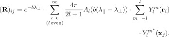
In the following, we assume a linear convolution model for the observed diffusion signal. According to this model, the response to any arbitrary angular distribution of fibers is equal to the sum of the individual responses to each fiber. More formally, the measured diffusion signal s(b,r) in each voxel is given by the spherical convolution
| (1) |
where b is the diffusion weighting factor, or “b‐value”, r is a unit (column) vector indicating the direction of the applied diffusion gradient, s
0 is the signal measured with no diffusion weighting (i.e.,  ), R(·,·,x) is the signal response to a single ideal fiber with orientation given by the unit (column) vector x, f(·) is a real‐valued function of the unit sphere describing the fiber orientation density (FOD), n(b,r) is additive measurement noise, and
  indicates integration of the unit sphere.
Note, in a typical HARDI experiment the data are collected using a discrete set of M evenly distributed and unique diffusion directions  with constant (non‐zero) b‐value, together with one or more measurements with b = 0 for normalization. Given N desired FOD reconstruction points on the surface
  , Eq. (1) can be written in matrix form
| (2) |
where s = [s(b,r 1)/s 0, …, s(b,r M)/s 0]T is a vector of normalized diffusion measurements, f = [f(x 1), …, f(x N)]T is a vector representation of the FOD, and R is an M × N linear convolution matrix relating the FOD to the normalized measurement data. Assuming an axially symmetric tensor model [Hsu and Mori, 1995] for the single‐fiber response function, the ij‐th entry of R can be written
| (3) |
where λ⟂ and λ∥ are the perpendicular and parallel diffusivities (ADC parameters) with respect to the fiber axis x j, with λ∥ ≥ λ⟂, and the inner product r x j is the cosine of the angle between the i‐th measurement direction and j‐th fiber axis. While the tensor model in Eq. (3) assumes the single‐fiber response function is Gaussian, non‐Gaussian or hybrid models of diffusion [Assaf et al., 2004] can also be used within this framework without any loss of generality.
SH Basis
The SH form a complete orthonormal basis for functions on the sphere much like the Fourier series form a complete orthonormal basis for functions in Euclidian space. In this section, we show how the convolution matrix R can be expressed in terms of the SH basis. While similar expressions appear in earlier works [Anderson, 2005; Tournier et al., 2004], the focus here is to extend this framework to derive an analytic expression for the efficiency of the minimum variance (maximally efficient) linear unbiased estimator for the FOD, which can subsequently be used for optimizing the HARDI acquisition.
We begin by expressing the response function in Eq. (3) as a sum of Legendre polynomials P l(·). Following [Anderson, 2005] [Appendix A, Eq. (36)] we can write
| (4) |
where the scalar coefficients can be computed by evaluating the integral
| (5) |
Notice, only even orders l = 0, 2, …, ∞ are considered in the expansion in Eq. (4) as the response function is symmetric around the fiber axis x j. Applying the Addition Theorem of Spherical Harmonics, we can write P l(r x j) in terms of the spherical harmonics Y (·) evaluated in the direction of each vector [Arfken and Weber, 2005]
| (6) |
where l and m are the order and degree of the spherical harmonic function, respectively, and * denotes the complex conjugate. Substituting Eq. (6) into Eq. (4) yields and expression for the ij‐th entry of R in terms of the SH
 |
(7) |
Enumerating all measurement and reconstruction points, the full convolution matrix can be written as a weighted superposition of matrices having the form
 |
(8) |
where it follows from Eq. (7) that
| (9) |
and the vectors of SH are
| (10) |
| (11) |
where H now denotes conjugate transpose.
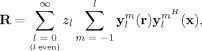
Equation (8) indicates that the convolution matrix can be represented by an infinite sum of even order SH, weighted by the coefficients z l. This is analogous to representing a delta function as an infinite series of Fourier basis functions. In practice, however, the number of diffusion directions, M, limits the maximum order that can be used in the expansion and thus the series must be truncated. Truncation of the SH series limits the angular resolution of the FOD much like truncating the Fourier series limits the bandwidth of reconstructed Cartesian signals.
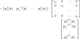
Consider, for example, a maximum order of L = 2, such that l = 0, 2. Expanding Eq. (8), we can write an expression for the truncated convolution matrix, denoted R L
| (12) |
 |
(13) |
| (14) |
where Y L(r), Z L, and Y (x) have dimensions M × p, p × p, and p × N, respectively, and p(L) = (L + 1)(L + 2)/2 is the number of terms (free parameters) in the SH series. For L = 2, p(2) = 6 and thus M should be greater than or equal to six to avoid an under‐determined set of equations. Therefore, the number of diffusion directions, in effect, determines the upper bound on the angular resolution of the FOD, such that p(L) ≤ M.
Inspection of Eqs. (12), (13), (14) yields several interesting properties of the FOD reconstruction problem. First, the SH form a natural basis for both the diffusion signal and the FOD, as it can be shown that the matrices Y L(r) and Y L(x) are unitary in the limit of M, N → ∞ [Nelson and Kahana, 2001]
| (15) |
| (16) |
Second, when expressed in terms of the SH basis, the diffusion signal is simply a weighted sum of the FOD signal and vice versa (i.e., Z L is diagonal) where the weighting is a function of the b‐value and ADC of the single‐fiber response model.
Estimation
Using the truncated convolution matrix, we can rewrite the signal in Eq. (2) as
| (17) |
Then, assuming the noise n is white with mean zero and variance σ, an efficient unbiased estimate of the FOD is provided by the ordinary least‐squares (OLS) solution to Eq. (17)
| (18) |
| (19) |
The OLS estimator for a linear model perturbed by white noise is optimal in the sense that it has the minimum variance among all linear unbiased estimators of the FOD. Note, however,  is technically an unbiased estimator of the projection of the true FOD onto the subspace spanned by the columns of Y
L(x). If part of the true FOD lies outside this subspace, for example,
is technically an unbiased estimator of the projection of the true FOD onto the subspace spanned by the columns of Y
L(x). If part of the true FOD lies outside this subspace, for example,  has higher angular frequency features not captured by the columns of Y
L(x), then
has higher angular frequency features not captured by the columns of Y
L(x), then  will be a biased (smoothed) estimate of the true FOD.
  can also be viewed as the truncated SVD solution.
Ideal Efficiency
As mentioned previously, the OLS estimator has the lowest variance among all linear unbiased estimators of the FOD. The goal here is to determine the MRI pulse‐sequence parameters which maximize the statistical efficiency. The efficiency of an estimator, which can also be viewed as a measure of the expected accuracy of the estimator, is typically defined as the reciprocal of estimator variance per unit scan time
| (20) |
where 〈·〉 is the expectation operator, and T is the total time required for the acquisition. For simplicity, and without loss of generality, in the remainder of this article we set T = 1 (i.e., assuming a constant scan time). Combining Eq. (19) with Eq. (20), we get the following expression for the efficiency of the OLS FOD estimator
| (21) |
Substituting the expression for the normalized signal in Eq. (17) into Eq. (21) and simplifying, we get
| (22) |
Finally, recalling n is white noise with mean zero and variance σ, we get the following expression for the efficiency of the OLS FOD estimator 
| (23) |
| (24) |
| (25) |
where the root mean squared (RMS) signal‐to‐noise ratio (SNR) is defined as  . Equation (25) together with Eq. (9) demonstrate how the ideal efficiency of the FOD estimate is a function of the b‐value, the ADC of the single‐fiber response, and the SNR at b = 0.
Realizable Efficiency
The expression for the efficiency of the OLS FOD estimator in Eq. (25) is ideal in the sense that it assumes a continuous sampling of measurement directions and FOD reconstruction points (i.e., as M, N → ∞) and pulse‐sequence parameters that are independent of the b‐value. In practice, however, the “realizable” efficiency of the FOD estimate depends on the efficiency of gradient sampling vectors in r, and the dependence of the echo‐time (TE) and repetition time (TR) on the b‐value. Taken together, we can write an expression for the realizable efficiency  of the FOD estimator (per unit scan time) as
| (26) |
where SNR0 is the SNR in RMS units at TE = 0 and b = 0, γi(r,x) is the i‐th singular value of the forward convolution matrix R(r,x) (given by Eq. (3)), and i = 1, 2, …, p is the spherical harmonic index for an L‐th order series expansion. The first term on the left hand side of Eq. (26) can be viewed as a reduction in efficiency due to constraints imposed by the pulse‐sequence and scanner hardware, while the second term on the right hand side of Eq. (26) can be viewed as the relative efficiency of the gradient sampling scheme. Note, the expression for the realizable efficiency  in Eq. (26) is no longer analytic, and requires computing the singular values numerically.
RESULTS AND DISSCUSION
Figure 1 shows a plot of the magnitude coefficients |z l| computed analytically using Eq. (9) for several different b‐values and fixed ADC parameters (λ∥ = 1.7 × 10⁻³ mm2/s and λ⟂ = 0.2 × 10⁻³ mm2/s). These ADC values are consistent with experimental estimates in the adult human brain [Pierpaoli et al., 1996], and are used throughout the remainder of this article. Notice the characteristic “staircase” pattern for each plot in the figure, where each “step” corresponds to a different spherical harmonic order l. The heights of the steps reflect the relative power to estimate features of the FOD spanned by the corresponding SH basis vectors. In all cases, power decreases with increasing SH order, reflecting an overall reduction in the ability to estimate higher angular frequency features of the FOD, irrespective of the b‐value. However, the rate at which power is lost is also dependent on the b‐value, with lower b‐values resulting in greater losses in power to estimate higher angular frequency components of the FOD.
Figure 1.
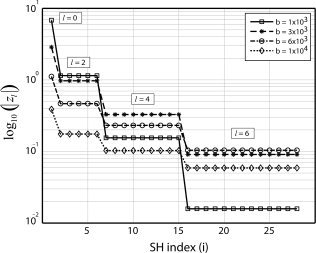
The magnitude of the coefficients |z l| are shown for four different b‐values (s/mm2) with a maximum SH expansion order of L = 6. The height of each step reflects the relative power to estimate features of the FOD spanned by the corresponding SH basis vectors. As the b‐value decreases, the relative power to estimate higher order angular frequency features of the FOD decreases.
Figure 1 can also be viewed as a plot of the analytic singular values of R L. Small singular values cause the inverse solution in Eq. (18) to become increasingly sensitive to small amounts of noise in the data. Several authors have introduced various linear and non‐linear regularization techniques to better condition both the FOD and ODF reconstruction problem, including Tikhonov regularization [Hess et al., 2006], Laplace‐Beltrami regularization [Descoteaux et al., 2007; Sakaie and Lowe, 2007], non‐negative least squares [Dell'Acqua et al., 2007; Jian and Vemuri, 2007; Tournier et al., 2007], and Maximum Entropy [Alexander, 2005]. These regularization techniques can decrease the mean squared error of the estimate, but this comes at a price of introducing estimator bias. The performance of each regularization method is critically dependent on whether the a priori constraints imposed on the solution are valid. The efficiency optimization approach presented here is valid for unbiased estimators where the estimation error is driven solely by the measurement error. The expression for the truncated SVD solution in Eq. (19) provides an optimum unbiased estimator of the projection of the true FOD into the subspace spanned by the columns of Y L(x).
The overall efficiency of the unbiased FOD estimator in Eq. (25) takes into account the relative power to estimate all the angular frequency components of the FOD by summing over I. Figure 2 shows a plot of the ideal FOD estimation efficiency E as a function of b‐value for L = 2, 4, 6, and 8. Again, note the decrease in efficiency for estimating FODs with higher order series expansions (and thus greater angular resolutions). Also, note the optimal b‐value which maximizes the efficiency depends on the expansion order, with higher order expansions requiring higher b‐values. The optimal b‐values which maximize the ideal efficiency of the FOD estimator using L = 2, 4, 6, and 8 are calculated to be approximately b = 1,500, 3,000, 4,600, and 6,200 s/mm2, respectively.
Figure 2.
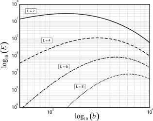
Ideal efficiency E of the OLS FOD estimator is plotted as a function of b‐value (s/mm2) for four different SH expansion orders L. Note, the exact value of the ideal efficiency is proportional to the SNR (see Eq. (25)), and thus the efficiency measure plotted here is in arbitrary units, assuming an SNR = 1. Optimal b‐values which maximize the ideal efficiency for L = 2, 4, 6, and 8 are calculated to be approximately b = 1,500, 3,000, 4,600, and 6,200 s/mm2, respectively.
Figures 1 and 2 illustrate the fundamental relationship between angular resolution, b‐value, and estimation efficiency. The theoretical angular resolution of a L‐th order SH expansion can be quantified using the angular point spread function (PSF) [Hess et al., 2006]. The full‐width at half maximum (FWHM) of the main lobe of the PSF determines the upper bound on angular resolution, and is inversely proportional to L. For L = 2, 4, 6, and 8, the theoretical angular resolution of the FOD estimator is approximately 110, 65, 46, and 36°, respectively [Hess et al., 2006]. Thus, in practice, increasing L would allow for resolving crossing fibers at increasingly finer separation angles, but as mentioned earlier, this comes at a price of decreasing efficiency. From Figure 2, one can see that using an expansion order of L = 6 at the optimal value of b = 4,600 is approximately 10 times less efficient than using an L = 4 expansion at its optimal value of b = 3,000 (1 × 10⁻²/9 × 10−4 ≈ 10), and 300 times less efficient than using a tensor description for the FOD (L = 2) at its optimal value of b = 1,500 (3 × 10⁻¹/9 × 10−4 ≈ 300).
In addition to the expansion order L, the b‐value also plays a critical role in determining the efficiency of the FOD estimator, especially when higher order expansions are used. For example, inspection of Figure 2 reveals that the efficiency for estimating the diffusion tensor (L = 2) is fairly constant between b = 500 and b = 3,000, but then falls off rapidly at higher b‐values. However, the efficiency for estimating crossing fibers (L ≥ 4) is more strongly dependent on the b‐value. Scanning at b = 1,000 using L = 4 would result in approximately 1/3 the efficiency of scanning at its optimum value of b = 3,000 (3 × 10⁻³/1 × 10−2 ≈ 1/3). This means one would have to collect three times as many diffusion directions, or equivalently, three times as many averages at b = 1,000 to achieve the same estimation accuracy as scanning at b = 3,000. In contrast, scanning at b = 2,000 would only result in a 10% drop in efficiency when compared to b = 3,000 (9 × 10⁻³/1 × 10−2 = 9/10).
While the expression for the ideal efficiency in Eq. (25) provides important insight into the FOD estimation problem, in practice, the realizable efficiency of the FOD estimator also depends on the arrangement of diffusion directions on the sphere, and scanner‐specific hardware constraints. Two of the most commonly used methods for selecting diffusion directions in MRI are to (1) minimize the electrostatic energy of pairs of equal and opposite points on the sphere, called the electrostatic repulsion (ER) model [Jones et al., 1999], and (2) to minimize the 1/r potential, which we call the minimum potential (MP) model (Hardin, Slone, and Smith, Spherical Codes, published electronically at http://www.research.att.com/~njas/electrons/index.html). Shown in Figure 3 are the relative efficiencies of both models for expansion orders L = 2, 4, 6, and 8. Also included is the efficiency of an “optimized” set of diffusion directions generated by searching for sampling arrangements which maximize Eq. (26). We refer to this new method for selecting diffusion directions as the “optimal efficiency” (OE) model. As illustrated in Figure 3, some sampling arrangements of the MP model are highly inefficient for estimating the FOD with L > 2 (i.e., for reconstructing crossing fibers). The ER model, in contrast, achieves nearly optimal efficiency for L ≤ 6, but has suboptimal efficiency for some sampling arrangements when using L = 8 and presumably for higher orders as well.
Figure 3.
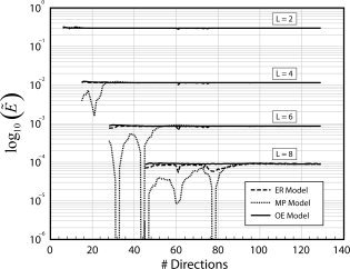
Effect of gradient sampling scheme on the realizable efficiency  of the FOD estimator. Shown are the relative efficiencies of the electrostatic repulsion (ER) model, minimum potential (MP) model, and the newly proposed “optimal efficiency” (OE) model. For each order L, the efficiency is calculated using their respective optimal b‐values and plotted in arbitrary units (term on the left hand side of Eq. (26) was set to 1). The FOD reconstruction vectors in x were chosen using a second‐order icosahedral sampling of the sphere (162 vertices).
Another important factor in the realizable efficiency of the FOD estimator is the minimal TE and TR allowed for a given b‐value. The effects of these scanner‐specific hardware constraints on the FOD estimation efficiency are illustrated in Figure 4. Shown in black are the efficiencies of a 51 direction acquisition (selected using the ER model) for multiple expansion orders, and using TE and TR values that are consistent with those prescribed on a General Electric Signa HDx 1.5T scanner (Waukesha, WI). Shown in gray are the efficiencies of this same acquisition using a fixed TE and TR calculated at b = 500 for reference. From Figure 4, one can see that the general effect of adjusting the TE and TR is to reduce the efficiency at higher b‐values, which results in slightly lower b‐values for optimal FOD estimation efficiency compared to the ideal case. For L = 2, 4, 6, and 8, the optimal b‐values which maximize the realizable efficiency on a Signa Hdx 1.5T system are approximately b = 1,000, 2,200, 3,600, and 5,200, respectively. Note that under these realistic conditions the relative efficiency for estimating crossing fibers using L = 4 at b = 1,000 now only results in about half the efficiency of scanning at its optimum value of b = 2,200, compared to 1/3 the efficiency in the ideal case. Also, it should be noted that while the actual change in efficiency will vary depending on the scanner specifics, the general trend will remain the same, i.e., a reduction in the efficiency at higher b‐values, and a subsequent decrease in the optimal b‐values required for maximally efficient FOD estimation.
Figure 4.
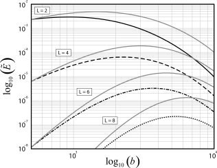
Effect of scanner‐specific hardware constraints on the realizable efficiency  of the FOD estimator. Black lines show the relative efficiencies of a 51 direction acquisition (selected using the ER model) using realistic TE and TR values that are consistent with those prescribed in practice. Gray lines show the relative efficiencies of the same acquisition using a fixed TE and TR calculated at b = 500. All efficiencies are calculated numerically using SNR0 = 1, T2 = 80 ms, and a second‐order icosahedral sampling for the FOD reconstruction vectors in x.
CONCLUSIONS
Several authors have used the SH basis to derive analytic expressions for both the FOD and ODF reconstruction problem. Here, we extend this framework and derive a simple analytic expression for the efficiency of the maximally efficient (minimum variance) linear unbiased estimator of the FOD. This expression highlights the important fundamental relationship between angular resolution, b‐value, and the expected accuracy of the FOD estimate per unit scan time. As expected, the FOD estimation efficiency decreases with increasing SH expansion order L (increasing angular resolution), and the relative efficiency at each order varies as a function of the b‐value. b‐values which maximize the efficiency under ideal conditions using L = 2, 4, 6, and 8 are calculated to be approximately b = 1,500, 3,000, 4,600, and 6,200 s/mm2, respectively.
However, the efficiency that can be realized in practice also depends on the arrangement of diffusion directions, and the scanner‐specific hardware limitations. We demonstrate how some commonly used methods for selecting diffusion directions can lead to suboptimal FOD estimation efficiencies, especially when higher order SH expansions are required, and we propose a new criterion for selecting diffusion directions based on optimizing the statistical efficiency. Finally, scanner‐specific limitations on the minimum TE and TR will generally cause a reduction in efficiency at higher b‐values, resulting in slightly lower b‐values for optimal FOD estimation when compared to the ideal b‐values.
REFERENCES
- Alexander DC ( 2005): Maximum entropy spherical deconvolution for diffusion MRI. Inf Process Med Imaging 19: 76–87. [DOI] [PubMed] [Google Scholar]
- Alexander DC, Barker GJ, Arridge SR ( 2002): Detection and modeling of non‐Gaussian apparent diffusion coefficient profiles in human brain data. Magn Reson Med 48: 331–340. [DOI] [PubMed] [Google Scholar]
- Anderson AW ( 2005): Measurement of fiber orientation distributions using high angular resolution diffusion imaging. Magn Reson Med 54: 1194–1206. [DOI] [PubMed] [Google Scholar]
- Arfken GB, Weber HJ ( 2005): Mathematical Methods for Physicists. 6th ed. San Diego: Academic Press; p 797. [Google Scholar]
- Assaf Y, Freidlin RZ, Rohde GK, Basser PJ ( 2004): New modeling and experimental framework to characterize hindered and restricted water diffusion in brain white matter. Magn Reson Med 52: 965–978. [DOI] [PubMed] [Google Scholar]
- Basser PJ, Pierpaoli C ( 1996): Microstructural and physiological features of tissues elucidated by quantitative‐diffusion‐tensor MRI. J Magn Reson B 111: 209–219. [DOI] [PubMed] [Google Scholar]
- Basser PJ, Mattiello J, LeBihan D ( 1994): Estimation of the effective self‐diffusion tensor from the NMR spin echo. J Magn Reson B 103: 247–254. [DOI] [PubMed] [Google Scholar]
- Dell'Acqua F, Rizzo G, Scifo P, Clarke RA, Scotti G, Fazio F ( 2007): A model‐based deconvolution approach to solve fiber crossing in diffusion‐weighted MR imaging. IEEE Trans Biomed Eng 54: 462–472. [DOI] [PubMed] [Google Scholar]
- Descoteaux M, Angelino E, Fitzgibbons S, Deriche R ( 2006): Apparent diffusion coefficients from high angular resolution diffusion imaging: Estimation and applications. Magn Reson Med 56: 395–410. [DOI] [PubMed] [Google Scholar]
- Descoteaux M, Angelino E, Fitzgibbons S, Deriche R ( 2007): Regularized, fast, and robust analytical Q‐ball imaging. Magn Reson Med 58: 497–510. [DOI] [PubMed] [Google Scholar]
- Frank LR ( 2001): Anisotropy in high angular resolution diffusion‐weighted MRI. Magn Reson Med 45: 935–939. [DOI] [PubMed] [Google Scholar]
- Frank LR ( 2002): Characterization of anisotropy in high angular resolution diffusion‐weighted MRI. Magn Reson Med 47: 1083–1099. [DOI] [PubMed] [Google Scholar]
- Hess CP, Mukherjee P, Han ET, Xu D, Vigneron DB ( 2006): Q‐ball reconstruction of multimodal fiber orientations using the spherical harmonic basis. Magn Reson Med 56: 104–117. [DOI] [PubMed] [Google Scholar]
- Hsu EW, Mori S ( 1995): Analytical expressions for the NMR apparent diffusion coefficients in an anisotropic system and a simplified method for determining fiber orientation. Magn Reson Med 34: 194–200. [DOI] [PubMed] [Google Scholar]
- Jansons KM, Alexander DC ( 2003): Persistent angular structure: New insights from diffusion MRI data. Dummy version. Inf Process Med Imaging 18: 672–683. [DOI] [PubMed] [Google Scholar]
- Jian B, Vemuri BC ( 2007): Multi‐fiber reconstruction from diffusion MRI using mixture of Wisharts and sparse deconvolution. Inf Process Med Imaging 20: 384–395. [DOI] [PMC free article] [PubMed] [Google Scholar]
- Jones DK, Horsfield MA, Simmons A ( 1999): Optimal strategies for measuring diffusion in anisotropic systems by magnetic resonance imaging. Magn Reson Med 42: 515–525. [PubMed] [Google Scholar]
- Le Bihan D ( 1995): Molecular diffusion, tissue microdynamics and microstructure. NMR Biomed 8: 375–386. [DOI] [PubMed] [Google Scholar]
- Nelson PA, Kahana Y ( 2001): Spherical harmonics, singular‐value decomposition and the head‐related transfer function. J Sound Vib 239: 607–637. [Google Scholar]
- Ozarslan E, Mareci TH ( 2003): Generalized diffusion tensor imaging and analytical relationships between diffusion tensor imaging and high angular resolution diffusion imaging. Magn Reson Med 50: 955–965. [DOI] [PubMed] [Google Scholar]
- Ozarslan E, Shepherd TM, Vemuri BC, Blackband SJ, Mareci TH ( 2006): Resolution of complex tissue microarchitecture using the diffusion orientation transform (DOT). Neuroimage 31: 1086–1103. [DOI] [PubMed] [Google Scholar]
- Pierpaoli C, Jezzard P, Basser PJ, Barnett A, Di Chiro G ( 1996): Diffusion tensor MR imaging of the human brain. Radiology 201: 637–648. [DOI] [PubMed] [Google Scholar]
- Sakaie KE, Lowe MJ ( 2007): An objective method for regularization of fiber orientation distributions derived from diffusion‐weighted MRI. Neuroimage 34: 169–176. [DOI] [PubMed] [Google Scholar]
- Tournier JD, Calamante F, Gadian DG, Connelly A ( 2004): Direct estimation of the fiber orientation density function from diffusion‐weighted MRI data using spherical deconvolution. Neuroimage 23: 1176–1185. [DOI] [PubMed] [Google Scholar]
- Tournier JD, Calamante F, Connelly A ( 2007): Robust determination of the fibre orientation distribution in diffusion MRI: Non‐negativity constrained super‐resolved spherical deconvolution. Neuroimage 35: 1459–1472. [DOI] [PubMed] [Google Scholar]
- Tuch DS ( 2004): Q‐ball imaging. Magn Reson Med 52: 1358–1372. [DOI] [PubMed] [Google Scholar]
- Tuch DS, Reese TG, Wiegell MR, Makris N, Belliveau JW, Wedeen VJ ( 2002): High angular resolution diffusion imaging reveals intravoxel white matter fiber heterogeneity. Magn Reson Med 48: 577–582. [DOI] [PubMed] [Google Scholar]
- Wedeen VJ, Hagmann P, Tseng WY, Reese TG, Weisskoff RM ( 2005): Mapping complex tissue architecture with diffusion spectrum magnetic resonance imaging. Magn Reson Med 54: 1377–1386. [DOI] [PubMed] [Google Scholar]
- White NS, Leergaard TB, Bolstad I, Bjaalie JG, D'Arceuil H, de Crespigny A, Dale AM. ( 2008): Quantitative histological validation of fiber‐orientation distributions based on high‐angular resolution diffusion imaging. Proc 16th Annual Meeting of the ISMRM, Toronto, Canada.
- Zhan W, Gu H, Xu S, Silbersweig DA, Stern E, Yang Y ( 2003): Circular spectrum mapping for intravoxel fiber structures baseds on high angular resolution apparent diffusion coefficients. Magn Reson Med 49: 1077–1088. [DOI] [PubMed] [Google Scholar]